Molecular Dynamics Simulation Methods Revised - Google Sites

Molecular Dynamics Simulation Methods Revised

H. Bekker

CIP-DATA KONINKLIJKE BIBLIOTHEEK, DEN HAAG Bekker, Hendrik Molecular Dynamics Simulation Methods Revised / Hendrik Bekker, - [S.l. : s.n.]([S.l.] : Febo Druk). - Ill. Thesis Rijksuniversiteit Groningen. - With ref. ISBN 90-367-0604-1 Subject headings: molecular dynamics / simulation / algorithms.

Omslag: Bart ten Hoonte/letter & lijn.

RIJKSUNIVERSITEIT GRONINGEN

Molecular Dynamics Simulation Methods Revised

Proefschrift ter verkrijging van het doctoraat in de Wiskunde en Natuurwetenschappen aan de Rijksuniversiteit Groningen op gezag van de Rector Magnificus Dr. F. van der Woude in het openbaar te verdedigen op vrijdag 14 juni 1996 des namiddags te 4.00 uur door

Hendrik Bekker geboren op 5 juni 1950 te Ee

Promotores: Prof.dr. H.J.C. Berendsen Prof.dr. N. Petkov

CONTENTS 1

2

3

Introduction 1.1 M.D. simulation in outline 1.2 The subjects of this thesis 1.3 Research goals : : : : : : 1.4 Discussion : : : : : : : :

: : : : : : : : : : : : : : : : : : : : : : : : : : : : : : : : : : : : : : : : : : : : : : : : : : : : : : : : : : : : : : : : : : : : : : : : : : : : : : : : : : : : : : : :

An Efficient Non-Bonded Force Algorithm 2.1 Introduction : : : : : : : : : : : : : : : : 2.2 Derivations : : : : : : : : : : : : : : : : : 2.2.1 Notation : : : : : : : : : : : : : : 2.2.2 Force derivations : : : : : : : : : 2.2.3 Virial derivations : : : : : : : : : 2.2.4 Neighbour searching : : : : : : : : 2.3 The Implementation : : : : : : : : : : : : 2.3.1 The algorithm : : : : : : : : : : : 2.3.2 The implementation : : : : : : : : 2.3.3 The machines used : : : : : : : : : 2.3.4 The test M.D. system : : : : : : : 2.3.5 The Test Runs : : : : : : : : : : : 2.3.6 Results : : : : : : : : : : : : : : : 2.4 Extensions : : : : : : : : : : : : : : : : : 2.4.1 Generalisation to other box shapes : 2.4.2 Applicability : : : : : : : : : : : : 2.5 Conclusion : : : : : : : : : : : : : : : : :

: : : : : : : : : : : : : : : : : : : : : : : : : : : : : : : : : : : : : : : : : : : : : : : : : : : : : : : : : : : : : : : : : : : : : : : : : : : : : : : : : : : : : : : : : : : : : : : : : : : : : : : : : : : : : : : : : : : : : : : : : : : : : : : : : : : : : : : : : : : : : : : : : : : : : : : : : : : : : : : : : : : : : : : : : : : : : : : : : : : : : : : : : : : : : : : : : : : : : : : : : : : : : : : : : : : : : : : : : : : : :

Unification of Box Shapes in Molecular Simulations 3.1 Introduction : : : : : : : : : : : : : : : : : : : 3.2 Defining primitive cells by a lattice and a metric : 3.3 Defining boxes by their edges : : : : : : : : : : 3.4 Constructing simple boxes : : : : : : : : : : : : 3.5 Translating particles between primitive cells. : : v

: : : : : : : : : : : : : : : : : : : : : : : : : : : : : : : : : : : : : : : : : : : : : : : : : :

1 1 8 10 11 13 13 15 15 16 18 21 22 22 25 26 27 27 27 29 29 30 31 33 33 36 39 42 45

vi

3.6 3.7

An example transformation of a simulation : : : : : : : : Related Topics : : : : : : : : : : : : : : : : : : : : : : : 3.7.1 Pressure scaling : : : : : : : : : : : : : : : : : : 3.7.2 Lattice reduction : : : : : : : : : : : : : : : : : : 3.7.3 Long range order : : : : : : : : : : : : : : : : : 3.7.4 How to set up a simulation : : : : : : : : : : : : : 3.7.5 Which box to use: the triclinic or the rectangular? : 3.8 Conclusion : : : : : : : : : : : : : : : : : : : : : : : : : Appendix A : : : : : : : : : : : : : : : : : : : : : : : : : : : Appendix B : : : : : : : : : : : : : : : : : : : : : : : : : : :

4

5

6

Constraint Dynamics 4.1 Introduction : : : : : : : : : : : 4.2 Zeroth order equations of motion 4.3 First order equations of motion : 4.4 Second order equations of motion 4.5 Discussion : : : : : : : : : : : : 4.6 Example applications : : : : : : 4.7 Conclusion : : : : : : : : : : : : Appendix C : : : : : : : : : : : : : :

: : : : : : : : : : : : : : : : : : : : : : : : : : : : : : : : : : : : : : : : : : : : : : : : : :

: : : : : : : : : : : : : : : : : : : : : : : : : : : : : : : : : : : : : : : : : : : : : : : : : : : : : : : : : : : : : : : : : : : : : : : : : : : : : : : : : : : : : : : : : : : : : : : : : : : : : : : : : : : : : : : : : : : : : : : : : : : : : : : : : : : : : : : : : : : : : : : :

Torsional-angle Potentials 5.1 Introduction : : : : : : : : : : : : : : : 5.2 Dihedral-angle force expressions : : : : 5.3 The virial of angle-dependent interactions Appendix D : : : : : : : : : : : : : : : : : : Appendix E : : : : : : : : : : : : : : : : : : Appendix F : : : : : : : : : : : : : : : : : :

: : : : : : : : : : : : : : : : : : : : : : : : : : : : : : : : : : : : : : : : : : : : : : : : : : : : : : : : : : : : : : : : : : : : : : : : : : : : : : : : : : : :

The Virial of Angle Dependent Potentials 6.1 Introduction : : : : : : : : : : : : : : : : : : : : : : : : : : : 6.2 Theory : : : : : : : : : : : : : : : : : : : : : : : : : : : : : : 6.2.1 The virial of interactions with angle dependent potentials 6.3 Simulated system and methods : : : : : : : : : : : : : : : : : 6.4 Simulation results : : : : : : : : : : : : : : : : : : : : : : : : Appendix G : : : : : : : : : : : : : : : : : : : : : : : : : : : : : :

: : : : : : : : : : : :

49 50 50 51 53 53 55 57 58 59 63 63 64 67 69 71 72 79 79 81 81 84 87 87 89 90 93 93 94 95 97 98 98

vii

7

8

Mapping MD on a Ring Architecture 7.1 Introduction : : : : : : : : : : : : : : : : : 7.2 M.D. simulation in more detail : : : : : : : : 7.2.1 Non Bonded Forces : : : : : : : : : 7.2.2 Bonded forces and constraints : : : : 7.3 Allocation of the NBF calculations on a ring : 7.4 Allocation of constraint- and BF calculations 7.4.1 Theory : : : : : : : : : : : : : : : : 7.4.2 Triplet and quadruplet allocation : : 7.5 Results and discussion : : : : : : : : : : : : 7.5.1 Test of Reduce on protein molecules 7.5.2 Discussion : : : : : : : : : : : : : : 7.6 Conclusion : : : : : : : : : : : : : : : : : :

: : : : : : : : : : : : : : : : : : : : : : : : : : : : : : : : : : : : : : : : : : : : : : : : : : : : : : : : : : : : : : : : : : : : : : : : : : : : : : : : : : : : : : : : : : : : : : : : : : : : : : : : : : : : : : : : : : : : : : : : : : : : : : : : : : : : : : : : : : : : : : : :

Delay Insensitive Synchronisation 8.1 Introduction : : : : : : : : : : : : : : : : : : : : : : : : : : 8.2 Constraint Molecular Dynamics simulation : : : : : : : : : : 8.3 SHAKE on a ring architecture : : : : : : : : : : : : : : : : : 8.4 The function ACWT implemented with the open collector bus 8.5 Discussion : : : : : : : : : : : : : : : : : : : : : : : : : : : 8.6 Conclusion : : : : : : : : : : : : : : : : : : : : : : : : : : :

: : : : : : : : : : : : : : : : : :

105 105 106 106 108 109 113 113 116 117 117 118 120 123 123 125 128 131 133 134

Samenvatting

137

Nawoord

143

Curriculum Vitae

145

Index

147

viii

ix

This thesis is based on the following papers: Chapter 2: “An efficient box shape independent non-bonded force algorithm for Molecular Dynamics”, H. Bekker, E.J. Dijkstra, H.J.C. Berendsen, M.K.R. Renardus, Molecular Simulation, 1995, Vol. 14, pp. 137-151. Chapter 3: Submitted to Journal of Computational Chemistry. Chapter 4: To be submitted. Chapter 5: “Force and Virial of Torsional-Angle-Dependent Potentials”, H. Bekker, H.J.C. Berendsen, W.F. van Gunsteren, Journal of Computational Chemistry, Vol. 16, No. 5, 527-533 (1995). Chapter 6: “The Virial of Angle Dependent Potentials in Molecular Dynamics Simulations”, H. Bekker and P. Ahlström, Molecular Simulation, 1994, Vol. 13, pp. 367-374. Chapter 7: “Mapping molecular dynamics simulation calculations on a ring architecture”, H. Bekker, E.J. Dijkstra, H.J.C. Berendsen, In Parallel Computing: From Theory to Sound Practice, ed. W. Joosen and E. Milgrom, pp. 268-279, IOS Press, Amsterdam, 1992. Chapter 8: “Delay insensitive synchronisation on a message-passing architecture with an open collector bus”, H. Bekker, E.J. Dijkstra Proceedings of PDP ’96, IEEE Comp. Soc. Press, 1996.

Other publications:

“Design of a transputer network for searching neighbours in M.D. simulations”, H. Bekker, M.K.R. Renardus, Microprocessing and Microprogramming, Vol. 30, 1-5, August 1990.

x

“GROMACS: a Parallel Computer for Molecular Dynamics Simulation”, H. Bekker, et al, Conf. Proc. Physics Computing ’92, pp. 252-256, World Scientific Publishing Co. Singapore, New York, London, 1993. “GROMACS: Method of Virial Calculation Using a Single Sum”, H. Bekker, et al, Conf. Proc. Physics Computing ’92, pp. 257-261, World Scientific Publishing Co. Singapore, New York, London, 1993. “Molecular Dynamics simulation on an i860 based ring architecture”, H. Bekker, E.J. Dijkstra, H.J.C. Berendsen. Supercomputer 54, X-2, 4–10, 1993.

1

INTRODUCTION

Molecular Dynamics (M.D.) Simulation is in principle very simple: the time development of a many particle system is evaluated by numerically integrating Newton’s equations of motion. But, as with most simple principles, many additional concepts and techniques have to be applied to make the main principle operational. The additional concepts and techniques are required, not because the main principle needs correction or refinement, but because a bare implementation of the main principle would result in very sluggish software without practical value. For that reason, from the outset in the fifties, much work has been done to turn a simple principle into a useful tool. In this thesis no new techniques are proposed, but existing techniques are revised. As a result, a number of concepts of M.D. simulation are simplified, and alternative implementations are proposed. In this chapter the main concepts of the M.D. simulation technique are introduced and an overview of this thesis is given. Also the goal of this thesis is formulated and some remarks are made about the way current M.D. implementations are created.

1.1 M.D. simulation in outline Main principle The main principle of M.D. simulation is as follows: given the system state S (t0 ), that is, the position r and velocity v of every particle (atom) in the system at time t0, subsequent states S (t0 + ∆t), S (t0 + 2∆t), : : :, are calculated by using Newton’s law F = ma. For accurate results small timesteps ∆t have to be used. To calculate S (t0 +(n + 1)∆t) from S (t0 + n∆t), first for every particle i, Fi(t0 + n∆t) is calculated. Fi (t0 + n∆t) is the sum of the forces on i as exerted by the other particles of the system at time t0 + n∆t. For every particle i the force Fi (t0 + n∆t) is then integrated to get the new velocity vi (t0 + n∆t). Using this velocity, for every particle i the new 1

Chapter 1 Introduction

2

position ri (t0 + (n + 1)∆t) can be calculated. See Figure 1.4. Integration A widely used, simple and numerically stable, integration algorithm is the leapfrog algorithm. In this algorithm particle positions are calculated at times t0 + n∆t and velocities at midpoints, i.e. at t0 + (n + 12 )∆t (this differs from the scheme in the previous paragraph where particle positions and velocities were both evaluated at t0 + n∆t). With tn t0 + n∆t, the formulas for leap-frog integration are vi (tn + ∆t=2)

=

vi (tn

∆t=2) + m 1Fi (tn )∆t ;

ri (tn + ∆t) = ri (tn ) + vi (tn + ∆t=2)∆t :

(1.1) (1.2)

Interaction forces Generally speaking, in an M.D. simulation the forces between particles only depend on particle positions, not on velocities. Usually, interactions are specified by giving an expression for the potential energy of the interaction, hence the force can be written as a gradient of the potential. Non-bonded interactions Two classes of interactions may be distinguished: non-bonded interactions and bonded interactions. Non-bonded interactions model flexible interactions between particle pairs. Two well-known non-bonded interaction potentials are the Coulomb potential and the Lennard-Jones potential. Using the convention that the distance between the particles i and j is defined as rij jrij j jri rj j, the Coulomb potential can be written as 1 qi qj : VCoul = 4 0 rij Here qi and qj are the charges of particles i resp. j . i, due to particle j is given by qiqj rij : Fij Coul: = 4 r3 0

ij

(1.3) The Coulomb force on particle

(1.4)

The Lennard-Jones potential is given by

0 !12 VL-J = 4" @ r ij

!1 6A ; rij

(1.5)

1.1 M.D. simulation in outline

3

VL-J ["] 6 5 4 3 2 1 0 -1 0

1

2

3

4

5

6

ri;j []

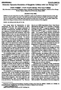
FIGURE 1.1 Lennard-Jones potential VL-J = 4"(( rij )12 ( rij )6). The depth of the potential well is determined by ", and the diameter of the particle by .

where " is a constant determining the depth of the potential well, and where 12 determines the diameter of the particle (see Figure 1.1). The term rij models

6

models an a strong repelling force at very short distances, and the term rij attracting force with a longer interaction range. Adding these two terms gives a potential well. The force of the Lennard-Jones interaction exerted on particle i by particle j is given by

Fij

=

0 !12 riVL-J (rij ) = 4" @12 r ij

6

!1 ! 6 A rij : rij rij2

(1.6)

Due to the ‘action= reaction’ principle (Newton’s third principle), the forces between two interacting particles are related by Fji

=

Fij :

(1.7)

So, the force between every particle pair i, j has to be evaluated only once instead of twice. The usual way to evaluate every interaction only once is to use the j > i criterion, i.e., to calculate explicitly the force on the particle with the highest particle number. The force on the other particle is calculated with (1.7). Bonded interactions Bonded interactions model rather strong chemical bonds, and are not created or broken during a simulation. For this reason, these interactions may be evaluated


4

by running through a fixed list of groups of particle numbers, where each group represents a bonded interaction between two or more particles. The three most widely used bonded interactions are the covalent interaction, the bond-angle interaction, and the dihedral interaction. The covalent interaction is a bonded interaction between two particles i and j with interaction potential V = 12 Kb (rij b0)2 : (1.8) This interaction may be thought of as a very stiff linear spring between i and j . The spring has a neutral length b0 and a spring constant Kb . The force of this interaction is given by Fi

=

Kb (rij b0)(rij =rij ) :

The bond-angle interaction is a three particle interaction between Figure 1.2a), with interaction potential V = 12 KΘ (Θ Θ0)2 ; with ! rij rkj : Θ arccos

rij rkj

(1.9)

i; j; k

(see

(1.10)

(1.11)

(Valid for small (Θ Θ0).) This interaction may be thought of as a torsion spring between the lines i; j and k; j . The spring has a neutral angle Θ0 and a spring constant KΘ . The dihedral-angle interaction V () is a four particle interaction between i; j; k; l (see Figure 1.2b) with an interaction potential V = V (). Two often used expressions for V are V = K 1 + cos(n ) and V = 12 K( 0)n 2 Z ; (1.12) where and 0 are constants. The definition of the dihedral angle is given by

sign() arccos(mˆ nˆ ) ; m rij rkj ; n rkj rkl ; rij n sign() j(r n)j ;

where rˆ rr .

ij

(1.13) (1.14) (1.15) (1.16)


5

m i

l

k

a)

n

φ

Θ j

b)

j

k

i

FIGURE 1.2 a: Bond-angle interaction. Θ is the angle between the lines i; j and k; j . b: Dihedral interaction with negative . m is normal to the i; j; k plane, n is normal to the j; k; l plane.

Cut-off radius and neighbour searching In principle, a non-bonded interaction exists between every particle pair. Because most of the CPU time of an M.D. simulation is spent in non-bonded force calculations, the greatest gain in performance can be achieved by efficiency improvements in this part. Two optimisations are widely applied: the use of a cut-off radius, and the use of neighbour lists. Earlier we proposed to evaluate all pair interactions, no matter how far the particles are separated. However, the main contribution to the total force on a particle is from neighbouring particles. Therefore, only a small error is introduced when only interactions are evaluated between particles with a distance less than a cut-off radius Rco . Choosing Rco so that for each particle 100 to 300 other particles are within cut-off radius gives a good balance between correct physics and efficiency. For a 104 system of 104 particles this makes the non-bonded force computation a factor 100 to 104 faster. 300 Still, when using a cut-off radius, all pairs have to be inspected to see if their separation is less than Rco . This is called neighbour searching. However, the timesteps made, are so small that particles travel only a very small distance during one timestep. In other words, the set of particles within Rco of a given particle hardly changes during one timestep. Therefore, only a small error is made when only every 10 or 20 timesteps all pairs are inspected to see if their distance is less than Rco . Pairs with a distance less than Rco are stored in so called neighbour lists

6


which are used the next 10 or 20 timesteps. In this way the all-pairs inspection every timestep is replaced by an all-pairs inspection every 10 or 20 timesteps at the cost of some memory space to store the neighbour list of every particle. Using Rco and a neighbour list, non-bonded force calculations still take about 70% of the total CPU time. Periodic boundary conditions Because of the limited CPU power, in current M.D. simulations typically 103 105 particles are involved. Single systems of this size suffer strongly from finite system effects. For example, due to the surface tension of water (or Laplace pressure), the pressure in a spherical droplet of water consisting of 2 104 molecules, will be approximately 275 bar. Many other anomalies are introduced by using small, single systems. Therefore, most simulations are done with periodic boundary conditions. This means that the simulation takes place in a computational box, which is virtually surrounded by an infinite number of identical replica boxes, stacked in a space filling way, all with exactly the same contents (see Figure 1.3). Only the behaviour of one box, the ‘central box’, has to be simulated; other boxes behave in the same way. When periodic boundary conditions are used particles may freely cross box boundaries. For each particle leaving the box, at the same instant an identical particle from an adjacent replica box enters the box at the opposite side. In an M.D. system with periodic boundary conditions particles are influenced by particles in their own box and particles in surrounding boxes. The shape of the computational box should be such that it can be stacked in a space filling way. For reasons of efficiency only convex boxes are used. In 3-D space there exist five box types with these properties: the triclinic box, the hexagonal prism, two types of dodecahedrons, and the truncated octahedron. A system with periodic boundary conditions is an infinite system, but has a crystal-like long range order. Ideally, one would like to have a system without this long range order. By choosing Rco not too large, the long range order effects are limited. Constraint dynamics Every timestep, during the force calculations, many types of interaction forces are evaluated: Coulomb forces, Lennard-Jones forces, covalent forces, etc. Some of these interactions are very rigid. The most rigid interaction in an M.D. simulation is the covalent interaction. This means that two particles having a covalent interaction, have an almost constant distance, or put in another way, two particles with a


FIGURE 1.3 boxes.

7

2-D Periodic Boundary Conditions. One box is surrounded by eight identical

covalent bond vibrate with a high frequency. The maximally allowed timestep used in an M.D. simulation is dictated by the allowed numerical drift of the integration algorithm, so it is dictated by the highest frequency in the system, and should be approximately 1=(40highest frequency). However, the behaviour of covalent interactions is not part of the physics of interest of an M.D. simulation because covalent vibrations are only weakly coupled to the other vibrations of the system. Leaving out frequencies above 1/4 to 1/2 the highest covalent eigenfrequency does not influence the outcome of an M.D. simulation. So, it is a waste of computer time to use a timestep based on covalent eigenfrequencies. For that reason, nowadays in most M.D. programs, the covalent interactions are handled using constraint dynamics, which means that the distance between particles with a covalent bond is kept constant. Then the timestep may be as high as 1/20 to 1/10 (highest frequency). In this way, the same time span of physics can be simulated two to four times faster. Because an atom may have covalent interactions with a number of atoms, substituting covalent interactions with length constraints will in general result in a set of connected length constraints with a, possibly cyclic, graph-like structure. In a typical M.D. system the number of constraints is of the same order as the number of particles. The introduction of length-constraints has no consequences for the force calculations, except of course that the forces of covalent interactions are not calculated.

8


However, the introduction of length-constraints has severe consequences for the algorithm in which Newton’s law is integrated, resulting in a matrix equation. As the rank of the matrix is the number of constraints in the system, for systems with many constraints, solving this equation directly is complex. There exists however a fast, iterative method, called SHAKE to solve the matrix equation. The special thing about SHAKE is that its iterative way of solving the matrix equation is directly reflected in iterative adjustments of pairs of particle positions. SHAKE is used as follows. Every timestep, the interaction forces, the new velocities, and new positions are calculated as if no constraints exist, except that no covalent interaction forces are evaluated. Particle positions obtained in this way do not fulfil the distance constraints between particles. Then SHAKE is invoked. In SHAKE, particle positions are iteratively corrected until all length-constraints are fulfilled within a predefined tolerance. So, at the end of every timestep many SHAKE iterations have to be done. Applications M.D. simulations are used to complement and to replace experiments in physics and chemistry. As such, M.D. has been used to study simple gases, liquids, polymers, crystals, liquid crystals, proteins, proteins in liquids, membranes, DNA-protein interactions, etc. For example, the equation of state (the p; T; V diagram) or transport phenomena, such as thermal conductivity of a gas, may be calculated by an M.D. simulation. For polymers M.D. has been used to calculate mechanical properties like compressibility and tensile strength. In the area of drug design, M.D. is used to calculate the free energy of a reaction. Nuclear Magnetic Resonance experiments give incomplete information about inter-atom distances; M.D. is used to refine these data. Many of the physical properties mentioned are not derived from one system state but as a time average over a long sequence of consecutive states. A much broader overview is given in [1].

1.2 The subjects of this thesis In this thesis, all the subjects mentioned in the previous section are revised, except neighbour searching and integration. So, the following subjects are discussed: nonbonded force calculations, bonded force calculations, constraint dynamics, and box shapes. Moreover, mapping M.D. simulation on a parallel computer with a ring

1.2 The subjects of this thesis

9

Neighbour Searching Neighbour lists

Bonded Force and Virial

Non-Bonded Force and Virial Non-bonded Forces

Bonded Forces

+ Total Forces

Integration Unconstrained Motion Unconstrained Positions

Constraint Dynamics

Positions

FIGURE 1.4 Main components of the M.D. simulation algorithm.

architecture is discussed. More precisely: In Chapter 2, an alternative method is presented to calculate non-bonded forces in systems with periodic boundary conditions. In Chapter 3 it is shown that the concept of ‘box shape’, as used in molecular simulations of systems with periodic boundary conditions, is superfluous. It is shown that every simulation can be done in a computational box with a simple shape.

10


In Chapter 4 the formalism of constraint dynamics is revised, so that it is suitable to study the (near) instantaneous behaviour of a system. In Chapter 5, alternative expressions of the torsional angle interaction are derived by using first principles of mechanics. In Chapter 6 it is shown that the scalar configurational pressure (virial) of angledependent interactions, is zero. This is also demonstrated with an M.D. simulation. In Chapter 7 it is shown how M.D. simulations may be mapped on a ring architecture, so that the communication related to the bonded force- and constraint interactions is minimised. In Chapter 8 a combined hardware and software solution is presented to speed up the synchronisation of constraint iterations on parallel computers with a sparse communication structure. Except for this chapter, all chapters of this thesis have been published (2,5,6,7,8), or will be submitted (3,4), so, are self-contained. For that reason the literature is given per chapter. The chapters in this thesis are not ordered chronologically but going from concepts to implementation. As a result, in some chapters reference is made to later chapters.

1.3 Research goals The research presented in this thesis stems from two questions: How can the different parts of the M.D. algorithm be reshaped, such that it becomes simpler and more efficient? How should the various parts of the M.D. algorithm be mapped on a ring architecture? Although we did not have the intention to do research in the field of physics, a number of new equations are derived, notably about the virial, bonded forces, and constraint dynamics.

1.4 Discussion

11

1.4 Discussion In the beginning, M.D. simulation was mainly used to study small artificial systems, but there was, and still is, a strong inclination to apply it to more realistic and more complex systems. All this with the intention to discover new, and explain known phenomena of molecular systems. This urge for results, together with the fact that M.D. software is designed and implemented by the M.D. community itself, has resulted in an evolutionary development of M.D. simulation software. This has the advantage that most simulations can be implemented quickly by adapting an existing implementation, but on the other hand runs the risk of evolutionary processes in general: the lack of an integral design. Once an idea has been implemented in some way, it is copied by other members of the M.D. community in their implementations, often without further critical reconsiderations. Besides the urge for results, also the apparent simplicity of the principles of M.D. simulation give the feeling that it is a waste of time to try to reshape M.D. simulation software. When one takes into account that M.D. simulation software was created by an evolutionary process, so, with the risk that errors in the software are passed on to later generations, it may come as a surprise that the physics of the great majority of simulations is correct. This is the case because the M.D. community is aware of the fact that the results of M.D. simulations are very sensitive to errors in the implementation. Therefore, before using a modified M.D. program for answering new questions, many test runs on old systems are done to validate the modified implementation. A significant amount of simulation time is spent on this. In contrast, as pointed out before, little time is spent on creating alternative implementations of parts of, or of the whole M.D. implementation. This thesis is an attempt to remedy this situation. In this thesis it is not tried to treat the M.D. simulation algorithms as a whole. Instead, some crucial concepts are reformulated and worked out separately. We there run the risk that more elegant concepts and more efficient algorithms, emerging from such an integral approach, are overlooked. We feel however that such an approach would be impracticable. In the first place because of the size of the problem. (The GROMOS M.D. simulation package is 1 Mbyte of FORTRAN code.) Secondly, because it is very difficult to find correctness preserving transformations, resulting in more efficient code. Thirdly, because, when the first two steps could be made with success, the resulting code would probably lack transparency. This is a major problem because much M.D. code is continuously modified by its users.

12


This thesis results from work directly and indirectly related with the GROMACS1 project. This project was started with the goal to design and construct a special purpose computer for M.D. simulations. Because this computer would have consisted of a long and wide unstructured pipeline with 100 ALU’s, registers, local memories, etc., it was important to use a specification of the M.D. algorithm that resulted in as simple as possible hardware. Therefore we started with analysing many parts of the M.D. algorithm. This proved to be a very important stage of the project, even when the project eventually was transformed into a project aimed at the design and implementation of a parallel computer for M.D. simulation, consisting of conventional processors. In the software of the resulting parallel computer, (a ring of 36 i860 processors) ideas presented in this thesis were implemented, notably those in the Chapters 2, 5, 6, 7. Although the activities were initially related to special purpose hardware, most of the ideas and concepts presented in this thesis may be used in M.D. implementations in general. The exceptions are the ideas in the Chapters 7 and 8. We have the feeling that besides the subjects treated in this thesis, some other parts of the M.D. algorithm are worth a critical reconsideration. To mention a few: Neighbour searching implemented with grid cells. The implementation of the force and energy evaluations with tables. The development of a very efficient, well documented M.D. kernel which can serve as a starting point for most implementations.

Literature [1] W.F. van Gunsteren and H.J.C. Berendsen, Computer Simulation of Molecular Dynamics: Methodology, Applications, and Perspectives in Chemistry. Angewandte Chemie Int. Ed., 29, 992 (1990).

(1)

GROMACS (GROningen MAchine for Chemical Simulations) was, in the period 1990– 1992, jointly developed by the RuG departments of Biophysical Chemistry and of Computing Science in STW project GCH88.1602.

2

AN EFFICIENT NON-BONDED FORCE ALGORITHM

A notation is introduced and used to transform a conventional specification of the non-bonded force and virial algorithm in the case of periodic boundary conditions into an alternative specification. The implementation of the transformed specification is simpler and typically a factor of 1.5 faster than a conventional implementation. Moreover, it is generic with respect to the shape of the simulated system, i.e. the same routines can be used to handle triclinic boxes, truncated octahedron boxes etc. An implementation of this method is presented, and the speed achieved on various machines is given. The essence of the new method is that the number of calculations of image particle positions is strongly reduced.

2.1 Introduction Conceptually, the M.D. simulationtechnique is simple: the time development of a many particle system is numerically evaluated by integrating the equations of motion. However, the inevitable introduction of time saving concepts as a cut-off radius, periodic boundary conditions, the nearest image criterion, and non-trivial box shapes makes realistic implementations complex, and makes it difficult to think in a clear way about alternative algorithms. In this chapter we will try to master this complexity by starting at the specification level and by introducing a notation which makes it easy to derive alternative specifications in a formal way from an initial specification. This proves to be simple and clear, and results in a surprising new non-bonded force (NBF) algorithm and a new virial algorithm. The new algorithms are generic with respect to the shape 13

14

Chapter 2 An Efficient Non-Bonded Force Algorithm

of the computational box, that is, the same NBF and virial algorithm may be used for the triclinic box, the truncated octahedron, and three more box shapes which can be stacked in a space filling way. Moreover, the implementation of the new algorithms, tested on a wide range of machines, proves to be faster than conventional implementations by at least a factor of 1.5. Besides these tangible results, our derivations also have the potential of giving a solid base to existing and new algorithms of other parts of the M.D. algorithms such as neighbour searching (NS) and bonded force calculations. In this chapter we will confine ourselves to the non-bonded and virial calculations, and do not address neighbour searching. As will be clear from the foregoing, we do not arrive at the new algorithms by transformations on the implementation level but by transforming a specification which is subsequently implemented rather straightforwardly in software. Three conditions should be fulfilled to make this method feasible: a suitable formal notation should be introduced, a correct initial specification should be available, and a set of transformation rules should be given. In [1] we used a notation which is rather clumsy, and which did not enable us to derive the results we present in this chapter. In contrast, the notation we use in this chapter lends itself very well for creating and manipulating specifications, and yet is simple. Also, in [1] we did not manipulate a specification but gave a proof at the operational level. In contrast, we now start with the specifications. The derivation of a correct specification for the NBF calculations is rather straightforward. Although a bit more complex this also is the case for the virial calculation. The set of transformation rules we apply is simple and their correctness is easily verified with a two-particle M.D. system. Following the usual M.D. practice, involving the minimum image convention, we assume that the cut-off distance Rco is such that particles in the central box only interact with particles which are in the central box and in directly adjacent boxes. The minimum image convention requires that every particle interacts with every other particle at most once, implying that Rco does not exceed half the length of the smallest image displacement vector. However, the algorithms we derive can be used as well for larger values of Rco . The algorithms derived in this chapter have been implemented on the GROMACS parallel computer for M.D. simulations [2,3]. However, because the GROMACS implementation also contains other innovations we will not discuss that implementation but a simpler one. In the next sections of this chapter we will discuss some properties of systems

2.2 Derivations

15

with Periodic Boundary Conditions (PBC), introduce a notation for particle positions and forces in PBC systems, and derive new force and new virial algorithms. We will discuss an implementation of these algorithms and compare the performance of a conventional implementation with the newly derived implementation. Finally we generalise the theory to other box shapes and discuss some other possible derivations of other parts of the M.D. algorithm.

2.2 Derivations 2.2.1 Notation To mitigate boundary effects in finite systems, most M.D. simulations are done on systems with PBC. An M.D. system with PBC consists of a central computational box with N particles, surrounded by an infinite number of translated identical image boxes, stacked in a space filling way. In the following we concentrate on the often used generalised cube or triclinic box, which is a chunk of space enclosed between six pairwise parallel planes. Other box shapes will be treated in Section 2.3. The box is defined by its three spanning vectors a ; b ; c. Every image box is a translated copy of the central box with a translation vector t given by t na a + nb b + nc c

na; nb; nc 2 Z) :

(

(2.1)

We define the minimum box size Lmin as the minimum distance between the parallel planes enclosing the box. Under the minimum-image convention we assume that Rco < 12 Lmin . To calculate the behaviour of the infinite system, only the behaviour of particles in the central box has to be calculated. When Rco < 12 Lmin , particles in the central box can only be influenced by particles in the central box and particles in the 26 directly adjacent boxes. So by numbering the boxes from 13 to 13 we are able to uniquely identify all boxes and particles we need to refer to. Using na; nb; nc of (2.1) we define the boxnumber k as

k = 9na + 3nb + nc

1 na ; nb ; nc

1;

(2.2)

so the central box has boxnumber 0. In Figure 2.1 a 2-D PBC system is shown with 4 k 4. Note that the box opposite to box k with respect to the central box has boxnumber k .


16

-2

1 Fi(j.-3)

-3

i

F(j.-3)i j

-4

0

4 Fi(j.3) i

-1

F(j.3)i j

3 2

FIGURE 2.1 2-D PBC system with boxes numbered -4 to 4, and with the relations between the four forces as given by equation (2.4). Note that box k is opposite of box k.

We will use the notation (j:k ) to indicate the particle with number j in box k . A single particle number j will indicate the particle with number j in box 0, that is, particle j is another notation for particle (j:0). The position of particle (j:k ) is denoted by r(j:k) and is given by the position of its parent particle in the central box plus the translation vector tk of the box k , so r(j:k)

=

rj

+ tk

:

(2.3)

The force exerted on particle (j:k ) by particle i in the central box is denoted by F(j:k)i . In the following we will often use the equalities (see also Figure 2.1) Fi(j:k)

=

F(i: k)j

=

F(j:k)i

=

Fj (i: k) ;

(2.4)

and tk

=

t k:

(2.5)

2.2.2 Force derivations In the usual implementation of a system of N particles the total force Fi on particle i is calculated as 13 N X X Fi = Fi(j:k) : (2.6) j =1 k= 13

2.2 Derivations

17

CP-COSP (i.1)

CP-COSP (i.3)

CP-COSP (i,0)

(a)

CP-COSP (i.4)

(b)

FIGURE 2.2 (a) Cut-off sphere in conventional way; dot is CP. (b) Cut-off sphere partitioned according to (2.8); dots are CP-COSPs.

Although we include the full sum over k , under the minimum image convention for each j only one k will contribute to the sum; all other image forces vanish because of the cut-off condition. Using (2.4), equation (2.6) can be rewritten giving Fi

=

N X 13 X j =1 k=

F(i: k)j :

When k runs from 13 to 13, commutative the order in which matter, so for Fi we may write Fi

=

N X 13 X j =1 k=

(2.7)

13

F(i:k)j :

k runs from 13 to 13. Because addition is k runs through the interval [13; 13] does not (2.8)

13

Let us elaborate on this expression because it is a central idea of this chapter. What (2.8) means is that the total force on particle i is calculated as a sum of forces on images of i (including the ‘null image’ in the central box) exerted only by particles in the central box. It is as if the usual cut-off sphere is partitioned by (image) box boundaries, and every cut-off sphere partition (COSP) is translated into the central box. With those COSPs which actually are translated, the central particle of the original cut-off sphere is also translated, resulting in central particles of partial cutoff spheres outside the central box. In Figure 2.2 both ways of calculating Fi are shown.


18

For further discussions we introduce the following notions. We call the conventional unpartitioned cut-off sphere ‘Cut-Off Sphere’ (COS), and partition the conventional cut-off sphere into ‘cut-off sphere partitions’ (COSPs). Also we keep calling the central particle (i:0) of the conventional cut-off sphere ‘central particle’ (CP), and call the central particle of a COSP, ‘central particle of cut-off sphere partition’ (CP-COSP). With neighbours of a CP we will mean all particles, both in the central box and image boxes, within Rco of that CP. With neighbours of a CP-COSP we mean all particles in the central box within Rco of that CP-COSP. Because Rco < 12 Lmin the neighbours of a given CP are located in at most eight boxes (including the central box). Therefore, every particle in the central box is split in at most eight CP-COSPs, each with its own neighbourlist. The total number of neighbours in these neighbourlists is equal to the number of neighbours in the neighbourlist of the corresponding CP, so the total number of NBF interaction calculations is not influenced by the use of the COSP method.

2.2.3 Virial derivations We define the virial tensor product Wij of an interacting pair of particles as Wij

rij Fij ;

(2.9)

where the tensorial direct product is defined as (u

v) = (u)(v) ; ; = x; y; z

(2.10)

and rij ri rj . As Erpenbeck and Wood [4] have shown (using a different notation), 1 W 2

N X i 1 X 13 1X ri(j:k) Fi(j:k) 2 i=1 j =1 k= 13

(2.11)

represents the internal Clausius virial in a periodic system. This expression takes each interaction for which i and j are both in the central box, into account only once. Interactions over the boundary of the central box occur pairwise (see Figure 2.1). Of these interactions only one is taken into account by (2.11). Equation (2.11) can be used to calculate the instantaneous pressure tensor P of the M.D. system as P=

1

V

W+

N X i=1

!

mivi vi ;

(2.12)

2.2 Derivations

19

where mi is the mass and vi the velocity of the ith particle, and V the volume of the system. The straightforward implementation of (2.11) involves its evaluation in the inner loop of the non-bonded force routine, which results in a significant CPU time consumption for this expression. We will therefore investigate how this expensive operation can be transformed in such a way that it can be moved to an outer loop. Using ri(j:k) = ri rj tk , we split ri(j:k) in (2.11) in three terms, ri , rj and tk , which gives =

W

N X i 1 X 13 X

ri Fi(j:k) +

i=1 j =1 k= 13 N X 13 i 1 X X +

i=1 j =1 k=

A+B +C:

N X i 1 X 13 X i=1 j =1 k=

rj

F j:k i + (

)

13

tk F(j:k)i

13

(2.13)

We will now show that the sum of A and B can be written as N X A + B = ri Fi : i=1 This follows from a rewriting of term B . Using F(j:k)i

B=

N X i 1 X 13 X i=1 j =1 k=

rj

=

Fj (i: k) (see (2.4)) gives

Fj i: k : (

(2.14)

)

(2.15)

13

Because k runs through values which are symmetric with respect to 0 we may replace k by k

B=

i 1 X 13 N X X i=1 j =1 k=

rj

13

Fj i:k : (

)

(2.16)

We may of course interchange the names i and j

B=

N jX1 X 13 X j =1 i=1 k =

ri Fi(j:k) :

Because (1 j N ) ^ (1 i j 1) implies (1 i < N ) ^ (i + 1 j P Pj 1 PN PN we get N j =1 i=1 (i; j ) = i=1 j =i+1 (i; j ). This gives

B=

(2.17)

13

N X N X 13 X i=1 j =i+1 k=

13

ri Fi(j:k) :

N ), (2.18)

20


Adding A and B and using Fi(i:k)

=

A+B = P

P

N X N X 13 X i=1 j =1 k=

13

0 gives

ri Fi(j:k) :

(2.19)

13 Using N j =1 k= 13 Fi(j:k) = Fi we get the required equation (2.14). To rewrite C we define gk as the total force on box k exerted by all higher numbered particles in the central box

gk

N X i 1 X i=1 j =1

F(j:k)i :

(2.20)

Using this definition C can be written as

C=

13 X

k=

tk gk :

Adding A, B and C we get W=

N X i=1

(2.21)

13

ri Fi +

13 X

k=

tk gk :

(2.22)

13

The last expression for W means that the virial may be calculated as if no periodicity P r F part), corrected with the P13 t g part. So, we have now exists (the N i i=1 i k= 13 k k reduced the double sum for W to a single sum plus a correction part C , which both can be cheaply evaluated in an outer loop of the NBF routine. Also, the calculation of gk , required for C , can be done in an outer loop of the NBF routine because, when P F is calculated using the COSP method, for every CP-COSP (i:k ) the sum N i=1 (j:k)i (2.8). (See the first statement on line 27 of the listing in Section 2.2.3.) The term C in (2.22) can be written in several ways. Which one is the most practical depends on the way forces are calculated. We will now derive some alternative expressions for C . By exchanging i and j in (2.20) and rewriting the double sum as was done in going from (2.16) to (2.18) we find that gk may also be written as N X N X gk = F(i:k)j : (2.23) i=1 j =i+1 The correction term C can also be written as

C=

13 X

k=

13

tk gk

=

13 X

k=

13

t k g k

=

13 X

k=

13

tk g0k

(2.24)

2.2 Derivations

where g0k

g0k

21

g k . Using (2.20) and (2.4) gives =

N X i 1 X i=1 j =1

F(j: k)i

=

N X i 1 X i=1 j =1

Fj (i:k)

=

N X i 1 X i=1 j =1

F(i:k)j :

(2.25)

A comparison of (2.23) and the last expression in (2.25 ) shows that the correction term C can also be written as

C=

13 1 X tk g00k : 2 k= 13

(2.26)

where

N X N X 00 gk F(i:k)j i=1 j =1

=

N X N X i=1 j =1

F(j:k)i :

(2.27)

This equation truly represents the total force of all particles in the central box on all particles in box k .

2.2.4 Neighbour searching In this subsection we will discuss the consequences of (2.8) on neighbour searching and the structure of neighbourlists. When non-bonded forces are calculated in the conventional way, that is with (2.6), for every CP a neighbourlist has to be constructed. When non-bonded forces are calculated in the new way, that is with (2.8), for every CP-COSP a neighbourlist has to be constructed. In contrast to the neighbourlist of a CP, the neighbourlist of a CP-COSP should only contain particles located in the central box. Using the nearest image criterion it is possible to calculate for every neighbour particle of a given CP its position, i.e. to calculate how the parent particle in the central box should be shifted to become the nearest image. With the new algorithm, instead of shifting neighbouring particles the CP-COSP is shifted. By using the nearest image criterion and the positions of particles in the neighbourlist of a given CP-COSP, it is possible in principle to calculate in which image box this CP-COSP should be located. This however is inefficient. It is much better to identify a CP-COSP by its particle number and its box identifier k . Doubling the memory requirements for CP-COSPs is relatively cheap compared to the memory requirements for the neighbourlists. In the rest of this chapter we shall mean by the COSP method the combination of (2.8) and the use of stored box identifiers of CP-COSPs in the CP-COSP list.

22


There is yet another reason for storing the box identifiers, which has to do with the integrity of charge groups. A charge group is a small group of particles which are involved in a common cut-off criterion, which means that all these particles or none of these particles are involved in a particular interaction. During NBF calculations all particles of a given charge group should undergo the same translation, even when this leads to a violation of the nearest image criterion. That is because a disrupted charge group would create a non-physical electric field over a long distance, leading to erroneous simulation results. The only way to prevent this situation is to calculate during neighbour searching the required translation of the charge group as a whole, and to use during NBF calculations this translation for all particles of the charge group, no matter what their actual position may become during subsequent timesteps. The identical translation requirement of charge group particles is not introduced by the COSP method. For the same reason as depicted above, in conventional implementations the translation of particles constituting a charge group should also be the same and kept constant between two successive neighbour searching calls.

2.3 The Implementation 2.3.1 The algorithm In this subsection we will show the outlines of an implementation of the M.D. algorithm with emphasis on the implementation of the new NBF method (2.8) and the new virial method (2.22). We will use a Pascal-like pseudo programming language which is capable of assigning vectors with one statement, returning a vector as a function result, etc. Some parts of the implementation are only outlined while other parts are given in more detail. The best way to understand this program is to first study the neighbourlist structure, that is, the data structures cp cosp and nl. To comment on this listing line numbers are used. After the listing the comments are given. To keep the listing clear, we use procedures without parameter list, which implies global access to data. Names used in this pseudo implementation are as close as possible to the symbols in the rest of this text. For the sake of simplicity we do not introduce differing particle types, charge groups, bonded forces, etc. 01: program MD; 02: constant 03: N = 10000; f= maximum nr of particlesg

2.3 The Implementation

04: MAX NR CP COSP = 8*N; 05: MAX NR INTERACTIONS = 160*N; 06: type vec = array [1..3] of real; 07: var 08: cp cosp: array [1..MAX NR CP COSP+1] of 09: record i, k, first: integer end; 10: nl: array [1..MAX NR INTERACTIONS] of integer; 11: r, v, F: array [1..N] of vec; 12: n, nr cp cosp, nr timesteps, lifetime of nl, i: integer; 13: t, g: array [ 13..13] of vec; 14: w: array [1..3, 1..3] of real; 15: procedure nbf; 16: var 17: a, b, i, j, k: integer; 18: f i k, fij, r i: vec; 19: begin 20: g := 0; F := 0; 21: for a:=1 to nr cp cosp do begin 22: i := cp cosp[a].i; k := cp cosp[a].k; 23: f i k:= 0; r i:= r[i] + t[k]; 24: for b:=cp cosp[a].first to (cp cosp[a+1].first) 1 do begin 25: j:= nl[b]; 26: fij:= force(r i,r[j]); 27: f i k += fij; F[j] -= fij; 28: end; fb loopg 29: g[k] += f i k; F[i] += f i k; 30: end; fa loopg 31: w := 0; 32: for i:=1 to n do w += r[i] F[i]; 33: for k:= 13 to 13 do w += t[k] g[k]; 34: end;fnbfg 35: begin fmaing 36: initialise; 37: for i:=1 to nr timesteps do begin

23


24

cp_cosp i

k

nl

first

[1]

[a] [a+1]

FIGURE 2.3 The neighbourlist structure of our pseudo implementation. In the array cp-cosp for every CP-COSP the particle number and box number is stored, as well as an index in the array nl. In the array nl the neighbours of the CP-COSP cp cosp[a] are located between cp cosp[a].first and (cp cosp[a+1].first)-1.

38: if (i mod lifetime of nl) = 1 then search neighbours; 39: nbf; 40: integrate; 41: end; fi loop g 42: end; fmaing Comments: 04: We have chosen the maximum number of CP-COSPs to be 8N, which works fine for small N. For large N, and a normal Rco , there are far less CP-COSPs because then many of the cut-off spheres intersect with less than eight boxes. 05: We assume a maximum average number of particles within Rco of 320. This results in an average of at most 160 non-bonded force calculations per particle. 08, 10: For storing neighbour information two arrays are used: cp cosp and nl. In cp cosp the particle number i and the box number k of every CPCOSP is stored. The neighbours of the CP-COSP described in cp cosp[a] are located in the array nl, at the places with index cp cosp[a].first, : : :, (cp cosp[a+1].first)-1. See Figure 2.3.


25

11: Position, velocity, and total force. 12: Actual number of particles, actual number of CP-COSPs during this lifetime of the neighbourlists, total number of timesteps to be done, number of timesteps to be done with the same neighbour lists, and loop variable. 13, 14: See (1), (20), and (9). t is updated every time the box dimensions change, e.g. by pressure scaling. 18: Accumulated force on CP-COSP i:k , interaction force introduced for the sake of efficiency, and image position of particle i introduced for the sake of efficiency. 20: Clear the arrays g and F. 26: The function force, not declared in this pseudo program, returns a vector valued result. 32, 33: See (22). We assume the existence of the tensorial product in our pseudo language. 36: Reads in the input, and initialises all relevant variables. 38: The procedure search neighbours is not declared in this pseudo program. Every time it is invoked it fills the variables cp cosp, nl, and nr cp cosp. 40: Using r, v, and F, the variables r and v are updated.

2.3.2 The implementation Based on the previous algorithm we have made an implementation of the M.D. algorithm with COSP and, for comparison purposes, an implementation without COSP (non-COSP). Both implementations were done in C.1 For a fair comparison the implementations only differ at those places where the COSP and non-COSP algorithms differ, that is, in the neighbour searching routine and the NBF routine. The main body of both implementations is exactly the same. In the implementation of both the COSP method and the non-COSP method we store particle numbers and box identifiers in the neighbourlists. As we explained before, this means that, in case of COSP, of every CP-COSP its number and box identifier k is stored. In case of non-COSP, the neighbourlist of every CP consists of particle numbers and box identifiers k . This makes our non-COSP implementation somewhat unconventional because in the NBF routine normally the nearest image criterion is used to determine the image box of particles. However, using the nearest image criterion for non-COSP, and the stored box identifier for COSP would lead to (1)

The complete set of sources can be obtained by anonymous ftp from ftp.cs.rug.nl in directory pub/moldyn.

26


an unfair comparison between the speeds of the COSP and non-COSP programs in favour of the COSP method. This is because the nearest image calculation is more expensive than the calculation of image positions using stored box identifiers. To minimise the time required for neighbour searching we use a grid search method. This means that a grid is constructed in the computational box, and that the particles are assigned to the appropriate grid cell before constructing the neighbourlist. Searching for neighbours of a particle is done by only inspecting the particles in its own and neighbouring cells. Experience shows that a grid size L = 12 Rco gives an optimal neighbour searching speed. Approximately one in four inspected particles is then in cut-off range. For M.D. systems as used in our tests, using a grid search NS CPU time ratio of 1 3. (See test results.) technique gives an approximate NBF Using an all-pairs neighbour searching technique gives a ratio of 2 1, i.e. the NS time is six times longer without the use of a grid search technique. The COSP method causes no problems with the implementation of the grid search technique. In order to allow a straightforward interpretation of the results we kept our test programs simple. That means that a single cut-off range was implemented, only one particle type was considered, no charge groups were implemented, no Bonded Forces (BF) were calculated etc.

2.3.3 The machines used We tested our implementations on a wide variety of machines to show that the type of machine does not influence the speed improvement we get. We also ran our program on the Convex and CM5, but because we did not vectorise or parallelise our code we do not include the results of those runs. We used the following machines and software: HP1 Hewlett Packard HP 9000-735; 128 Mb memory; 200 Mb swap; gcc 2.3.3. HP2 Hewlett Packard HP 9000-720; 64 Mb memory; 200 Mb swap; gcc 2.3.3. IRIS Silicon Graphics SGI 210; 32 Mb memory; 48 Mb swap; gcc 2.4.3. i860 Intel i860XR; 40 Mhz; 8 Mb memory; hcc. i486 Intel 80486 running SCO Unix; 66 Mhz; Local bus; 32 Mb memory; 64 Mb swap; gcc 2.4.3. SUN SPARC station SLC; 16 Mb memory; 40 Mb swap; gcc 2.3.3.


27

2.3.4 The test M.D. system All tests were done on an argon-like system with PBC consisting of 8000 particles in a cubic box with sides 21.0 units long (reduced density ? = 0:863). The potential used is the dimensionless Lennard-Jones potential

V (r) =

4:0=r6 + 4:0=r12 :

(2.28)

For all tests the initial system conditions are identical. Initially particles are distributed over the box by placing them at the grid points of a cubical grid, and giving them small random displacements. Initial velocities are Gaussian distributed with random direction, such that the net system momentum is zero. Rco was chosen such that there were either 100 or 300 neighbours on average within cut-off range. The neighbourlist was updated every 10 timesteps. Having 100 neighbours means that on average approximately 50 NBF evaluations per particle are done. This number of particles within cut-off is typical for particles in a protein, which are only interacting with other protein particles. The other Rco is typical of water atoms which are only interacting with other water atoms. The timestep was the same for all simulations, and all runs had a length of 10 timesteps.

2.3.5 The Test Runs To keep the test circumstances on all machines as much as possible constant the same operating system (UNIX) and the same files were used for all tests. This means that the same compiler, the gcc compiler, was used for all tests on all machines. The exception was the i860 for which no gcc compiler was available to us. On that machine we used the Intel High C compiler instead. The timing was done by clocking the two parts of the inner loop using the system clock. Again, the i860 was the exception because in this case the timing was done using the clock of a connected transputer. We used single processor programs; no use was made of the multiprocessor capabilities some of the machines have.

2.3.6 Results In Table (2.1) the results of the measurements done for both the non-COSP and COSP program for both cut-offs, with their respective number of neighbours, are given as


28

the number of steps per second and the percentage of time spent on non-bonded force calculations for each run. It is easy to deduce from the table the execution time of the NBF routine.

NON-COSP neighbours

100

COSP 300

100

300

system

speed

%NBF

speed

%NBF

speed

%NBF

speed

%NBF

HP1 HP2 IRIS i860 i486 SUN

0.64 0.27 0.26 0.17 0.097 0.031

(73) (74) (79) (73) (79) (84)

0.21 0.087 0.083 0.050 0.030 0.010

(76) (79) (82) (72) (82) (86)

0.89 0.40 0.38 0.25 0.16 0.049

(64) (68) (81) (70) (83) (85)

0.31 0.14 0.12 0.076 0.052 0.015

(68) (72) (84) (73) (82) (87)

TABLE 2.1 Comparison of the speed in steps per sec. of the conventional (non-COSP) and the COSP algorithm, including neighbour searching once per 10 steps, performed on various machines. The tests were done for two cut-off ranges (100 and 300 particles within Rco ). The COSP implementation is consistently 1:5 faster than a conventional implementation. In parenthesis the percentage of total step time spent in NBF. The rest of the time was taken up by NS.

From these results it is clear that the COSP implementation is consistently almost 1:5 times faster than the non-COSP implementation. This is the most important conclusion to be drawn from the table. Some further observations can be made. As expected, on all machines the number of timesteps per second decreases by a factor of three when the number of particles within cut-off range is increased by a factor of three. The percentage of time spent in NBF calculations is lower for the high performance machines. Because the rest of the time is spent in neighbour searching this means that neighbour searching is relatively more efficient on simpler machines. However, in all tests, irrespective of the machine, the times spent on neighbour searching and on NBF calculations for the COSP implementation are less than the corresponding times for the non-COSP implementation. The differences in hardware speeds also account for the differences in time spent in

2.4 Extensions

29

force calculations between COSP and non-COSP. In neighbour searching the COSP way the percentage of integer calculations is much higher than in the non-COSP way.

2.4 Extensions 2.4.1 Generalisation to other box shapes In the previous sections of this chapter we assumed that the computational box, and consequently image boxes, are triclinic. When we limit ourselves to convex figures there are however five different regular figures, called parallelohedra, whose translated replicas can be fitted together along whole faces to cover the whole space just once [5]. In increasing order of complexity they are: the cube (six squares), the hexagonal prism (six rectangles and two hexagons), the rhombic dodecahedron (twelve rhombi), the elongated dodecahedron (eight parallelograms and four hexagons), and the truncated octahedron (six squares and eight hexagons). Of course the affine transforms of these figures can also be stacked in a space filling way, which for example generalises the cube to the triclinic shape. All five shapes consist of pairwise parallel planes, so for every one Lmin can be defined analogous to the definition in Section 2.2.1. Of these five figures the cube requires the largest minimal number of surrounding image systems to be fully enclosed by these image systems. That is because the cube has six faces in common with surrounding systems, twelve vertices, and eight edges, giving a total number of surrounding systems of 26. The derivations in Section 2.2 were done for a triclinic box but they also hold for the other four box shapes because (2.4) (2.5) and (2.6) do not depend on the box shape. All the information concerning the place of image boxes is stored in t. So, when the COSP method is used literally the same NBF and virial routine may be used for all five box shapes. For the time being, only the neighbour searching routine is different for every box shape, as is the routine which resets particles in the box previous to neighbour searching. In a next chapter we will however show how these five figures can be mapped on a rectangular box. This will make neighbour searching and resetting particles also generic with respect to the box shape. Combining the COSP method with the generic neighbour searching and resetting algorithm will result then in a completely box shape independent M.D. algorithm.

30


2.4.2 Applicability In this section we make a few remarks about other possible applications of the methods we presented in earlier sections of this chapter, and a few remarks about implementing only a part of the methods proposed. Large cut-off. In the usual M.D. simulation practice Rco < 12 Lmin . For a part this is for physical reasons; to mitigate effects introduced by PBC a particle should interact with at most one image of a particle. Another reason is that with existing M.D. software it is difficult to identify multiple images of a given particle. With our method this is no problem because CP-COSPs are identified by a particle number and a box identifier k . In that way it is possible to represent multiple occurrences of the same parent particle within Rco of a given particle. In our implementation this would only mean a longer t and g array, and require a modified neighbour searching routine. Interactions over the central box boundary in a half space. In the usual M.D. simulation practice and also in our implementation particles in the central box interact with particles in the central and surrounding boxes, where surrounding boxes may have both positive and negative image identifiers k . With the notation and transformation rules we introduced in Section 2.2 it is however possible to derive a specification and consequently an implementation in which particles in the central box interact with particles in the central and surrounding boxes, with only non-negative image identifiers k . That is because for every interaction of a particle in the central box with a particle in an image system there exists a translated but otherwise identical interaction over the opposite box boundary (see Figure 2.1). Which interaction is evaluated in the NBF routine is a matter of choice, so the neighbourlists may be constructed in such a way that only interactions which cross the boundary to image systems with a non-negative k are entered into the lists. At this moment we do not see a useful application for an algorithm of this kind but maybe it is useful on a future exotic parallel computer. We mention an algorithm of this kind to show how useful formal methods as introduced in this chapter are to derive alternative M.D. algorithms. Mixed COSP and conventional implementations. From practical considerations one may wish to implement only certain parts of the COSP method. For example, one may wish to use (2.22) for calculating the virial in an otherwise conventional implementation. Also, one may wish to use the COSP method without the introduction of explicit box identifiers, or the other way around, to use explicit box

2.5 Conclusion

31

identifiers but not the other parts of the COSP method. Although not impossible in principle, implementations of this kind are inconsistent and clumsy. We recommend that the COSP method should be adopted as a whole or a conventional implementation should be used.

2.5 Conclusion Specifying and transforming the NBF and virial routine in case of PBC, and the introduction of the explicit image identifier k has roughly speaking three results. First, the formal derivation gives existing and new M.D. algorithms a solid base. Yet, the derivations are so simple that the contact between the derivation and the actual M.D. algorithm is never lost. This gives a better insight in what is going on in the NBF and virial algorithm. Secondly, the algorithms we derived, are significantly (1:5) faster than conventional algorithms, without penalty on applicability. Thirdly, the algorithms are generic with respect to the box shape. The same NBF and virial routine may be used for triclinic, truncated octahedron box shapes etc., without any loss of speed. Only the neighbour searching routine has to know what box shape is being used. The character of the NBF and virial routine is generic because the COSP method strongly reduces the number of images to be calculated, and thus makes it possible to store explicit image identifiers k of the few remaining images instead of recalculating images during the NBF calculations. In short, using COSP in MD programs will make these programs run faster with roughly a factor 1:5 compared with conventional implementations, and will make the NBF routine general with respect to box shape.

Acknowledgements We thank H. Keegstra and B. Reitsma for useful discussions, and Biomos b.v. for giving us the opportunity to discuss ideas presented in this chapter at the Burg Arras Biomos ’93 meeting.

32


Literature [1] H. Bekker, H.J.C. Berendsen, E.J. Dijkstra, S. Achterop, R. v. Drunen, D. v.d. Spoel, A. Sijbers, H. Keegstra, B. Reitsma, and M.K.R. Renardus, in Conf. Proc. Physics Computing ’92, 257-261, World Scientific Publishing Co. Singapore, New York, London. [2] H. Bekker, H.J.C. Berendsen, E.J. Dijkstra, S. Achterop, R. v. Drunen, D. v.d. Spoel, A. Sijbers, H. Keegstra, B. Reitsma and M.K.R. Renardus, in Conf. Proc. Physics Computing ’92, 252-256, World Scientific Publishing Co. Singapore, New York, London. [3] H. Bekker, E.J. Dijkstra, H.J.C. Berendsen, Supercomputer 54, X-2 (1993), 4-10 [4] J.J. Erpenbeck, W.W. Wood, in Statistical Mechanics B. Modern Theoretical Chemistry, ed. B.J. Berne (Plenum, New York, 1977), Vol. 6, 1-40. [5] L. Fejes Tóth, Regular Figures, Pergamon Press, London, 1964, 114-119.

3

UNIFICATION OF BOX SHAPES IN MOLECULAR SIMULATIONS

In molecular simulations with periodic boundary conditions the computational box used, may have five different shapes: triclinic, the hexagonal prism, two types of dodecahedrons, and the truncated octahedron. In this chapter we show that every molecular simulation, irrespective of the shape of the initial computational box, can be done as a simulation in one of the other ones, i.e. we show that in a preprocessing phase a simulation formulated in one particular box can be transformed into a simulation in another box such that the simulation in the new box is exactly identical to the simulation in the original one. This means that every molecular simulation may be done in the same type of box. Because the triclinic box is the easiest one to implement, we pay special attention on how to transform the other four box types into triclinic boxes. As a consequence, simulations in the often used truncated octahedron are superfluous; they may be done in a much simpler way in a triclinic box.

3.1 Introduction To mitigate finite system effects most molecular simulations are done on systems with periodic boundary conditions (P.B.C.). This means that the computational box is surrounded in a space-filling way by replica boxes, with identical content. In terms of the crystallographic Bravais lattices we consider only triclinic systems, i.e systems without symmetry elements. In [1] it is proven that in 3-D space there are five convex1 box types (see Figure 3.1) (1)

This property is not strictly necessary, but image calculations would become very complex for a non-convex box.

33

Chapter 3 Unification of Box Shapes in Molecular Simulations

34

PCT1

PCT4

PCT2

PCT3

PCT5

PCT5R

FIGURE 3.1 Instances of the triclinic box, the hexagonal prism, two types of dodecahedrons, the truncated octahedron, and the most regular instance of the truncated octahedron, in this chapter designated by PCT1, PCT2, PCT3, PCT4, PCT5, and PCT5R respectively.

that can be stacked in a space filling way, i.e. that there are five possible types of boxes which may serve as a computational box: the triclinic box, the hexagonal prism, two types of dodecahedrons, and the truncated octahedron. For short we will designate these box types by PCT1, PCT2, PCT3, PCT4, and PCT5, where PC stands for ‘Primitive Cell’, and T stands for ‘Type’. The notion ‘primitive cell’ will be explained later. The rectangular instance of PCT1 will be designated by PCT1R and the most regular instance of PCT5 by PCT5R. In the M.D. world, PCT5R is often called ‘the truncated octahedron’, but as we will show later it is only the most regular instance of a broader class of boxes. In the early years of molecular simulation PCT1 was used. Later PCT3 was introduced [9], and then PCT5R [8]. In current implementations of molecular simulation algorithms, the shape of the computational box has to be taken into account at many places in the algorithm, notably in neighbour searching, in non-bonded force calculations, in bonded force calculations, and in the part in which particles are reset into the box. For the computational boxes PCT2, : : :, PCT5, which have a complex shape, calculating the

3.1 Introduction

35

position of image particles outside the box as a function of their position in the box, is complex. For this reason, in most molecular simulation packages only a limited set of box shapes has been implemented. E.g. in the molecular dynamics package GROMOS [2] only a limited instance of PCT1 and PCT5R have been implemented. In this chapter we will show that every molecular simulation which is formulated in one of the boxes PCT1, : : :, PCT5, can be transformed into a simulation in any one of the other boxes. So, a simulation, formulated in PCT2, : : :, PCT5 can be transformed into a simulation in PCT1 or PCT1R. These transformations can be done in a preprocessing stage of a molecular simulation, so the actual simulation can take place in for example PCT1 or PCT1R, including neighbour searching, nonbonded force calculations, bonded force calculations, resetting particles into the box, pressure scaling, etc. The simulation in PCT1 and PCT1R is exactly identical to a simulation of the initial, untransformed system. So, for example, the number of particles and interactions to be evaluated is exactly the same in all cases. The structure of this chapter is as follows. In Section 3.2 we define the shape of PCT1, : : :, PCT5 in an algebraic way by a lattice and an alternative metric. Using this representation we derive the main theorem of this chapter. The lattice-and-metric way of defining PCT1, : : :, PCT5 is not suitable for geometrical considerations. Therefore, in Section 3.3 we introduce a different, but equivalent representation of PCT1, : : :, PCT5. Using this representation, we show that PCT1, : : :, PCT4 are degenerate instances of PCT5, and we show show how a tiling of the space with PCT5 defines a lattice. In Section 3.4 we define a PCT1 and a PCT1R in terms of a given PCT5, such that PCT1 and PCT1R define the same lattice as PCT5. Because PCT1, : : :, PCT4 are degenerate instances of PCT5, the same expressions may be used to define a PCT1 and a PCT1R in terms of PCT1, : : :, PCT4.2 In Section 3.5 we show how to map particles from one box into another one. As an example, in Section 3.6 we show how a simulation, formulated in PCT5R, is transformed into PCT1 and PCT1R. The fact that every simulation, formulated in some box may be transformed into a simulation in an other box, clarifies a number of unresolved matters. Notably the pressure scaling of simulations in an PCT2, : : :, PCT5 box, controlling the long range order of a molecular systems, and the maximum allowed cut-off radius. These (2)

Obviously, transforming PCT1 into PCT1 is an identity transformation. But because of the generic character of the algorithms we propose, we do not have to exclude PCT1 from our algorithms.


36

matters and more will be discussed in Section 3.7. The methods presented in this chapter may be used to transform existing molecular simulations, formulated in PCT2, : : : PCT5, into a simulation in for example PCT1 and PCT1R. That is, however, not the best way to set up a new simulation because then, complex boxshapes are still used to set up a simulation. In Subsection 3.7.4 it is shown how to set up a new simulation without using complex boxes. We feel that the methods as presented in this chapter to do molecular simulations in a simple box, together with the efficient method presented in [3], will result in faster and simpler molecular simulation software with a wider range of features. All this, is brought about, not by improving existing implementations, but by revising the basic concepts of M.D. simulation.

3.2 Defining primitive cells by a lattice and a metric In 3-D space, a lattice L is the set of points

L(

K; L; M )

n1

K

+

n2 L + n3M ;

with n1 ; n2 ; n3

2 Z;

(3.1)

where K , L, and M are three independent vectors, called the basis vectors. We define a lattice vector as a vector connecting two lattice points, so, because the origin is a lattice point, lattice vectors are also given by (3.1). Two points, 1 and 2, are called corresponding points when their positions are related by r1

+ lattice

vector = r2 :

(3.2)

In Euclidean space the squared distance d2 (p1 ; p2 ) between two points p1 and p2 is given by

d2 (p1 ; p2 ) = (p1

T I (p 1

p2 )

p2 )

:

(3.3)

where I is the unit matrix. The Euclidean distance function satisfies the general conditions of a distance function

d(p1 ; p2 ) > 0; if p1 6= p2 ; d(p1 ; p2 ) = d(p2 ; p1 );

d(p1 ; p1 ) = 0; d(p1 ; p2 ) d(p1 ; p3 ) + d(p3 ; p2 ); 8p3:

(3.4) (3.5)

However, the Euclidean distance function is not the only one meeting these conditions. Every function defined as

d2 (p1 ; p2 ) = (p1

T m (p

p2 )

1

p2 )

;

(3.6)

3.2 Defining primitive cells by a lattice and a metric

FIGURE 3.2 functions.

37

Two primitive cells defined by the same lattice but two different distance

with m a positive definite matrix, satisfies (3.4), (3.5). (A matrix m is called positive definite when mT

=

m and xT m x > 0;

for all x 6= 0 :

(3.7)

Note that m is by definition symmetric.) We can use a lattice and a distance function to partition the whole space in primitive cells in the following way. To every lattice point p belongs a primitive cell PC , defined so that every point in PC is closer to p than to any other lattice point. This is the well known Voronoi or Wigner-Seitz construction [10], using a more general metric. In Figure 3.2 two 2-D examples are given of a primitive cell defined by the same lattice but by different distance functions. It has been proven that by giving a lattice and a metric, the 3-D space is partitioned into five types of primitive cells [6]. These are the triclinic box, the hexagonal prism, two types of dodecahedrons, and the truncated octahedron, i.e. PCT1, : : :, PCT5. In this way every primitive cell is uniquely determined by a lattice and a distance function. I.e. every possible computational box can be described by giving a lattice and a metric, and the other way around. In our definition of a lattice, the origin is a lattice point. We will designate a primitive cell in general by PC, and a primitive cell centred around the origin by PC0. The primitive cells PCT1, : : :, PCT5, PCT1R, and PCT5R, centred at the origin, are denoted as PC0T1, : : :, PC0T5, PC0T1R, and PC0T5R. In each primitive cell is a unique lattice point, which we will often call the centre of PC. A primitive cell defined in this way is an open set of points, because, in our definition of a primitive cell, we do not consider points with the same distance to two lattice points. This would mean that a point with equal distance to two or more lattice points is not in any primitive cell at all. For molecular simulation this is undesirable;

38


every point in the infinite PBC system should belong to exactly one (image) box. Therefore it is necessary that we define a primitive cell as a half open, half closed set of points, so that tiling the space with primitive cells covers every point of space exactly once. How this is implemented is of no importance in later discussions. There we will simply take a primitive cell as a half open half closed set of points. Using the lattice-and-metric way to define primitive cells, we will now derive some theorems about primitive cells, culminating in the main theorem of this chapter. We present these derivations in an informal style. A molecular system with P.B.C. is in principle an infinite system because every (image) box is surrounded by replica boxes. With an infinite system we will mean the set of particles, not the boxes. This gives the following definition: Definition 1 Two infinite molecular systems IS and IS0 are called identical when for every particle in IS there is an identical particle in IS0 at the same position, and when for every particle in IS0 there is an identical particle in IS at the same position. Theorem 1 A primitive cell does not contain two corresponding points. Proof: Assume that a primitive cell PC contains two corresponding points i and j . This means that i and j are closer to the centre of PC than to any other lattice point, while ri rj is a lattice vector. Primitive cells are centred around lattice points, so the relative position of primitive cells are lattice vectors. This means that shifting a point, belonging to some primitive cell, over a lattice vector will bring this point to another cell. However, shifting i over the lattice vector ri rj brings it to j , which is in the same cell. This contradiction implies that the first assumption is wrong. Theorem 2 A lattice L and a metric m define the cell PC0. Then, for every point in space, there is a corresponding point in PC0. Proof: A tiling of the space with PC covers every point of the space. So, every point p will fall in some PC. This PC is shifted over a lattice vector with respect to PC0. Shifting p over minus this lattice vector will bring this point into PC0. According to Theorem 1 this is the only translation over a lattice vector which brings p into PC0. Consequently, when we have two primitive cells defined by the same lattice but different metrics, for every point in one cell there is a corresponding point in the other one, and the other way around. The central theorem of this chapter is:

3.3 Defining boxes by their edges

39

Theorem 3 A lattice L and a metric m define a primitive cell PC0. PC0 contains particles. Tiling the space with PC0 gives an infinite system IS. The same lattice L and another metric m0 define PC0 0. According to Theorem 2, the particles from PC0 are brought into PC0 0 by shifts over lattice vectors. Tiling the space with PC0 0 gives an infinite molecular system IS0. Then IS and IS0 are identical.

Proof: The position of a particle in PC0 and its position in PC0 0 only differ by a lattice vector (Theorem 2). IS is created by tiling the space with PC, that is, by locating a tile PC at every lattice point. IS0 is created by locating a tile PC0 at every lattice point. So, particles are only shifted over lattice vectors. Because tiling means shifting over all possible lattice vectors, every particle in IS coincides with a particle in IS0. So far for theorems. We will now investigate how many parameters are required to specify the most general primitive cell, being PCT5. In 3-D space, a lattice is defined by giving three independent vectors, so, by giving nine numbers. A distance function is fully defined by giving a symmetric 3 3 matrix m, so, by giving six numbers. However, we do not use the distance function to measure distances but only to compare distances. So, for our purpose it does not matter whether we use m, or m multiplied with a uniform factor. In this way, the number of parameters required to define the distance function reduces from six to five. Therefore, we arrive at nine plus five is fourteen parameters to describe a primitive cell. Describing a primitive cell in this way means that its shape and its orientation in space is determined, but not its position. A last remark, about the diameter of a PC. The diameter of a PC is the maximum of the distance between any pair of points belonging to PC. It can be shown that for any lattice L, potentially the diameter of the primitive cell is unbounded. Using a lattice and metric to define a primitive cell is conceptually elegant, but not very well suited for geometrical considerations. In the next section we will use another way to describe PCT1, : : :, PCT5, which makes it possible to think in a more geometrical way about these box types.

3.3 Defining boxes by their edges It has been proved [4] that a primitive cell, as introduced in the previous sections, is centrally symmetric, and that it is bounded by pairs of parallel faces. A face is a centrally symmetric hexagon or parallelogram. The edges of a primitive cell consist


40

d

e

g f a

c b

b

c f g d FIGURE 3.3

e

An instance of PCT5 defined by the six edges b; c; d; e; f; g.

of groups of parallel lines. Using this last property, we come to our way of describing a primitive cell. We describe PCT5 by giving its edge vectors b; c; d; e; f; g (see Figure 3.3). These six vectors completely define PCT5 because it consists of 36 edges, which can be grouped into six groups of six parallel edges each. When the vectors b; c; d; e; f; g were independent, PCT5 would have 6 3 = 18 degrees of freedom. However, the

g

PCT5

0

f

PCT4

cde lin.dep.

0

PCT3

e

PCT2

0

PCT1

FIGURE 3.4 PCT5, PCT4 created by letting g ! 0 of PCT5, PCT3 created by letting f ! 0 of PCT4, PCT2 created by letting jcdej ! 0 of PCT3, PCT1 created by letting e ! 0 of PCT2. Fat lines go to zero.

3.3 Defining boxes by their edges

41

vectors defining the hexagonal planes should be coplanar. This gives four constraint conditions: jc; e; gj = 0, jb; d; gj = 0, jc; d; f j = 0, jb; e; f j = 0. So, PCT5 can be described by 18 4 = 14 parameters, which corresponds with the number found in the previous section. The number of degrees of freedom of PCT4, : : :, PCT1 can be obtained by degenerating PCT5 as shown in Figure 3.4. To degenerate PCT5 into PCT4, only the length of the vector g should go to zero because the direction of g is not free. That is because g is the intersection of the planes defined by the vectors c; e and b; d. So, PCT4 has one degree of freedom less than PCT5, i.e. 14 1 = 13. In the same way PCT4 can be degenerated into PCT3 by letting f ! 0. Again, because f is the intersection of two planes, defined by the vectors c; d and b; e, only the length of f can be changed. So, PCT3 can be described by 13 1 = 12 parameters. PCT2 can be obtained from PCT3 by choosing the vectors c; d; e to be linearly dependent. This condition brings the number of degrees of freedom of PCT2 to 12 1 = 11. PCT1 can be obtained from PCT2 by e ! 0. The vector e is not completely free; it should be in the plane defined by the vectors c; d. So it has two degrees of freedom. This brings the number of degrees of freedom of PCT1 to 11 2 = 9. This number of degrees of freedom is what may be expected expected from a triclinic box. The whole process of going from PCT5 to PCT1, can be concisely written as PCT5

g

!0

j j!0 !0 ! PCT4 !!0 PCT3 — — ! PCT2 ! PCT1 : f

cde

e

(3.8)

This shows that PCT1, : : :, PCT4 are degenerate instances of PCT5, that PCT1, : : :, PCT3 are degenerate instances of PCT4, etc. Put in an other way one can say that PCT5 is the generic space filler. Therefore, in the following paragraphs we only consider transformations of PCT5. Some properties of PCT5, : : :, PCT1 are given in Table 3.1. Again something about notation. Until now we only have been speaking about different box types. In this and the following sections different ways to describe boxes are introduced. We will denote a box described by the vectors b; c; d; e; f; g as PCDg. The g stands for ‘general’ because this is the most general way to describe a primitive cell. The box PCDg can be of any type because some vectors may be chosen zero or linearly dependent. Later, two other ways to describe boxes will be introduced. Analogous to our previous notation, the box PCDg centred at the origin is designated by PC0Dg. A few words about the absolute position of boxes. The centre of symmetry of PCDg is half way the line connecting two opposite points of PCDg. The opposite


42

PCT5

PCT4

PCT3

PCT2

PCT1

14 6 8 36 24 14

12 8 4 28 18 13

12 12 0 24 14 12

8 6 2 18 12 11

6 6 0 12 8 9

nr. faces nr. rhombi nr. hexagons nr. edges nr. vertices degr. freedom TABLE 3.1

Some properties of PCT5, : : :, PCT1.

vertices marked by a dot in Figure 3.3 are connected by the vector (b + c + d + e + f + g ). We will use the vector a to give the position of PCDg. Centring PCDg around the origin means that a should have the value 1 (b + c + d + e + f + g ) ; 2 so, by applying this expression, a PCDg becomes a PC0Dg. a

=

(3.9)

3.4 Constructing simple boxes Theorem 3 was about box shapes and particle positions. Let us first focus only on box shapes. In Theorem 3 it was shown that every box PC0 0, which generates the same lattice as PC0, may be used to construct an infinite molecular system IS0, identical to IS. In this section we will propose two boxes, a triclinic and a rectangular one, generating the same lattice as an initial box PCDg. We will first derive expressions for the lattice vectors of the lattice generated by a box PCDg. We start by considering an PC0Dg. As can be seen in Figure 3.5, the centres of replica boxes, fitted to this box are at the positions K

;

= (g + d + e + f )

L

;

= (g + b + e)

M

= (f

c

+ e)

:

(3.10)

With some patience, it can be verified that every other replica box fitted to the original box, is shifted over an integer linear combination of K; L; M . So, the whole space can be tiled with copies of the original box centred at the lattice points defined by K; L; M . As long as the vectors b; c; d are linearly independent the expressions (3.10) for K; L; M are meaningful, i.e. they also hold for the boxes PCT1,: : :,PCT4.

3.4 Constructing simple boxes

43

g

e b f e d

g

FIGURE 3.5 The vectors K; L; M defined by PCT5 with three replica boxes fitted along whole faces. It can be seen by inspection that K = (g + d + e + f ), L = (g + b + e), M = (f c + e) (not shown).

With the lattice vectors K; L; M we can easily define a primitive cell which generates the lattice defined by K; L; M , namely the triclinic box spanned by the lattice vectors themselves (see Figure 3.6). We will call a box defined by the vectors K; L; M , ‘PCDKLM’, and ‘PC0DKLM ’ when it is centred at the origin. We will use these names only in relation with a given box PCDg or a given lattice K; L; M . The boxes PCDKLM and PC0DKLM can only be of the type PCT1. Now we will introduce a rectangular box that generates the lattice defined by the

K L

M

FIGURE 3.6 The most trivial primitive cell of a lattice is the triclinic box PCT1, spanned by the basis vectors of the lattice.


44

V

L

K

U

FIGURE 3.7 A rectangular primitive cell PCDUVW (fat lines), and the the PCDKLM from which it is derived (thin lines), both centred around the same point.

vectors K; L; M . First the vectors K; L; M have to be reordered such that

j j j j j j: K

L

(3.11)

M

As we will show in Appendix B this simplifies some calculations in a later stage. Using the reordered vectors K; L; M , the vectors U; V ; W spanning a rectangular primitive cell are given by a Gram-Schmidt orthogonalisation process (see Figure 3.7) U

=

K

;

V

=

L

(L

ˆ ˆ

K )K

;

W

=

M

(M

ˆ K

L)K

ˆ ; L

(3.12)

ˆ c bc . The first expression needs no comment. The with aˆ aa and with b jbcj second expression means that V is perpendicular to K , so to U , and that it is in the plane defined by K and L. The third expression means that W is perpendicular to the plane defined by K and L, which implies that it is perpendicular to the plane defined by U and V . Analogously with the nomenclature already introduced, we will call the primitive cell described by the vectors U; V ; W PCDUVW or PC0DUVW. We will use these names only in relation with a given box PCDKLM or a given lattice K; L; M . Boxes should be centred at lattice points, so, should be stacked with relative shifts over the lattice vectors K; L; M . This means that in a tiling with the boxes PCDUVW, the boxes are not fitted along whole faces (see Figure 3.8). This last fact looks a bit special because with the primitive cells PCT1, : : :, PCT5, the space could be tiled by fitting these boxes along whole faces. A way out of this seemingly strange property of PCT1R is by taking it as a PCT5, with some of its faces in the

3.5 Translating particles between primitive cells.

45

FIGURE 3.8 The box PCT1R has to be centred at lattice points, resulting in a tiling that is seemingly not a tiling along whole faces. However, by taking PCT1R as a special instance of PCT5, this tiling may be taken as a face to face tiling. This is indicated by the fact that every box PCT1R is directly surrounded by 14 boxes, just like a tiling with a general PCT5.

same plane. In general PCT5 has contact along whole faces with 14 adjacent boxes, just like PCDUVW. So, by taking PCT1R as a special instance of PCT5 the anomaly is explained. Let us now briefly look at the volume of the various primitive cells we encountered. For a given lattice, defined by the vectors K; L; M , the volume of the primitive cells PCDg, PCDKLM , and PCDUVW is the same, and is given by determinants jK; L; M j and jU; V; W j. That is because to every lattice point belongs one primitive cell, no matter the shape of this primitive cell. With this we have finished the discussion on how to transform one type of primitive cell into another type. In the following section we will see how the particles in one primitive cell should be mapped into another primitive cell.

3.5 Translating particles between primitive cells. In Theorem 2 it was shown how to map particles from a primitive cell PC0 into a primitive cell PC0 0, both defined by the same lattice but a different metric: particles should be shifted from PC0 to PC0 0 over lattice vectors. In this way, the infinite molecular system generated by tiling the space with PC0 0 is identical to the infinite system generated by tiling the space with PC0. In principle, that is all there is to

46


mapping particles between primitive cells. The only remaining problem is to find for every particle the lattice vector bringing the particle from PC0 into PC0 0. In general, it is difficult to give an explicit expression for the required shift. Therefore, we will not use a direct method to find the required lattice vector, but try lattice vectors. This can be done because it is possible to give an upper bound of the order of the required shift, i.e. if the required shift is n1 K + n2 L + n3 M it is possible to give an upper bound of n1; n2 ; n3 . For example, in Appendix A it is proved that particles in PC0Dg have to undergo at most first order shifts to be translated into PC0DKLM, i.e. 1 n1 ; n2; n3 1. This way of determining the required lattice vectors is not the most efficient, but it is general. Because the process of translating particles from PC0 into PC0 0 is done in a preprocessing stage of the actual molecular simulation, the inefficiency is no problem. The algorithm for translating particles We will now discuss two algorithms to move particles from PC0Dg into the related PC0DKLM . We assume that we have a boolean function INPC0D2(r), which determines whether r is in the box PC0DKLM. With this function, and using the boundedness of the required translations, the algorithm to move a particle from PC0Dg into PC0DKLM is as follows: procedure PutIntoPC0D2(var r: vector); fr is shifted from PC0D1 into PC0D2g constant maxOrder = 1; fsee Appendix Ag var n1, n2, n3: integer; s: vector; fk,l,m are vectors, globally declared and initialisedg begin for n1 := -maxOrder to maxOrder do begin for n2 := -maxOrder to maxOrder do begin for n3 := -maxOrder to maxOrder do begin s := n1*k + n2*l + n3*m;fvector operatorsg if InPC0D2(r + s) then begin fvector operatorsg r := r + s; exit(PutIntoPC0D2); end; fif InPC0D2g

3.5 Translating particles between primitive cells.

47

end; ffor n3g end; ffor n2g end; ffor n1g end; fputIntoPC0D2g

This implementation of PutIntoPC0D2 is not very efficient because translations over first order shifts are tried first, while the shift over zero is the most probable one. Later we will encounter a case where maxOrder is more than one, which results in even more inefficiency. Therefore we will now show a more efficient implementation of PutIntoPC0D2. The inefficiency is removed by first trying the most probable shift, which is the zero shift. Then, the second most probable shifts are tried, which are shifts over lattice vectors in the first layer around the origin. Then, if max order > 1, the shifts over lattice vectors in the third layer are tried, and so on. procedure PutIntoPC0D2(var r: vector); var j, a, b, maxRadius: integer; procedure tryShiftingIntoBox(n1, n2, n3: integer); var shift: vector; fnote vector operationsg begin shift := n1*k + n2*l + n3*m; if InPC0D2(r+shift) then begin r := r + shift; exit(PutIntoPC0D2); end; fifg if inbox1(r -- shift) then begin r := r - shift; exit(PutIntoPC0D2); end; fifg end; ftryShiftingIntoBoxg beginfPutIntoPC0D2g maxRadius := 100; for j := 0 to maxRadius do begin f try further and further away g

48


for a := j to j do begin for b := j to j do begin tryShiftingIntoBox(a, b, j); end; ffor bg end; ffor ag for a := j to j do begin for b := j+1 to j 1 do begin tryShiftingIntoBox(a, j, b); end; ffor bg end; ffor ag for a := j+1 to j 1 do begin for b := j+1 to j 1 do begin tryShiftingIntoBox(j, b, a); end; ffor bg end; ffor ag end; ffor jg FatalError(’Max radius overflow.’); end; fPutIntoPC0D2g

Comments on this pseudo code: Note that we use vector operators in this code. The code consists of three similar blocks, each consisting of a nested loop over a and b. In the first block all lattice points in the top and bottom plane of a cube with ‘radius’ j are visited. In the second block the lattice points in the left and right plane are visited, and in the third block the lattice points in the front and back plane are visited. In Appendix B it is shown that particles in PC0DKLM have to undergo at most second order shifts to be translated into PC0DUVW. This means that the procedure proposed in this subsection can also be used for that case, with of course the exception that in the algorithms maxOrder:=2. Later we will encounter a case where the maximum order of the translation is unbounded, but still zero shifts are the most probable ones with decreasing probability outwards. For that case, the second implementation of the procedure PutIntoPC0D2 is the only one that can be used because in the first implementation infinite translations would be tried first.

3.6 An example transformation of a simulation

49

3.6 An example transformation of a simulation In the M.D. simulation package GROMOS, two box shapes are implemented: PCT1R, and PCT5R. In this section, as an example application of the theory, we will show how a simulation, formulated in PCT5R, can be transformed into a simulation in PCT1 and PCT1R. We will assume that PCT5R is centred at the origin, so, that it is actually a PC0T5R. PC0T5R is obtained by cutting away pieces of a cube with edge lengths h. The cutting away of pieces is done with the Voronoi, or Wigner-Seitz construction, using the Euclidean metric. This results in a PC0T5R with edge vectors b; c; d; e; f; g given by

0 B b = B @

0

0 B e = B @

1 4

1 4 1 4

1 4

0

1 C hC A; h 1 hC hC A;

0 1 0 B C c = B @ h CA; h 0 1 h B C f = B @ 0 CA; h 1 4

1 4

1 4

1 4

Applying (3.10) gives the vectors K; L; M

0 1 h B C K = B @ 0 CA; 0

0 B L = B @

1 2 1 2 1 2

1 hC hC A; h

0 1 h B C d = B @ h CA ; 1 4

1 4

0 B g = B @ 0 B M = B @

0

1 hC 0 C A: h 1 4

0

V

0 B =B @

0 1 2 1 2

1 C hC A; h

0 B W = B @

(3.14)

1 4

1 2 1 2

+ 12

Applying (3.12) gives the vectors U; V ; W

1 0 h C B U = B @ 0 CA;

(3.13)

1 2 1 2

+ 12

1 hC hC A: h 1 hC hC A: h

(3.15)

(3.16)

It can be checked that the volume of each of these three figures (PC0T5R, PC0T1, PC0T1R) is 12 h3 . In Figure 3.9a PC0T5R is shown with a (fancy) spherical molecule. The molecule is mapped into PC0T1 according to Theorem 2 (see Figure 3.9b). The fact that the molecule is ‘cut into pieces’ in PC0T1 indicates that the atoms of the molecule are shifted over different lattice vectors when translated from PC0T5R into PC0T1. PCT5R is the most regular instance of PCT5. Consequently, as can be seen in (3.15), the lattice vectors K; L; M are also special, i.e., to create image particles


50

a)

b)

FIGURE 3.9 a: PC0T5R with a (fancy) spherical molecule. b: PC0T1 derived from PC0T5R, with the molecule mapped into it. It is instructive to copy b) on a transparent sheet, and to fit this copy at various faces to its original. It can then be seen that the molecule is reconstructed.

surrounding the original box PCT5R, the particles in the box have to undergo regular shifts. The regularity of these shifts is exploited in [5] to calculate in a simple way the required shifts. Quite appropriately, this shift pattern is called the ‘checkerboard’ periodic boundary condition. However, this shift method is only applicable to PCT5R, and the actual simulation is still done in PCT5R. We have made some software available3 as both Turbo Pascal and C code with executables. In DEM1 the primitive cells PCT1, : : :, PCT5 can be (randomly) generated, and visualised (in X). In DEM2 the process of moving particles from PC0T5R into PC0DKLM and PC0DUVW is implemented. DEM2 can thus be used by the M.D. community to transform existing simulations, formulated in PCT5R, into a simulation in PC0DKLM and PC0DUVW.

3.7 Related Topics 3.7.1 Pressure scaling The most general pressure of an molecular system can be represented by a 3 3 tensor P. The pressure per dimension is defined as a vector (Pxx , Pyy , Pzz ), and the scalar pressure P is defined as

P 13 trace(P) : (3)

(3.17)

Can be obtained by anonymous ftp from ftp.cs.rug.nl in directory pub/mdbox.

3.7 Related Topics

51

In many M.D. simulations, every now and then the M.D. system, that is, the box and particle positions, is scaled depending on the most recently calculated pressure. In case the computational box is triclinic, it is well known how to scale the system [11]: in case only the scalar pressure is calculated, the box and particles are scaled in every dimension with the same factor. In case the pressure is calculated per dimension, the system is scaled per dimension, proportional to the components of the pressure vector. In case the full tensorial pressure is used, the system is scaled by multiplying all particle position and box vectors with the scaled pressure tensor. As a result of the the last two types of pressure scaling, the angles of the system may change. With the notions developed in this article, it is clear how to scale the system when the computational box is one of PCT2, : : :, PCT5 and a pressure scaling per dimension or a full tensorial pressure is used. Then, just as in the case of a triclinic box, the system may be scaled by scaling box vectors and particle positions per dimension, resp. by multiplying box vectors (b, : : :, g ) and particle positions with a scaled tensor P. This is because the infinite M.D. system may be taken as a tiling of the space with one of PCT2, : : :, PCT5 but just as well as a tiling with PCT1.

3.7.2 Lattice reduction Until now our attention has been focussed on transforming simulations in a complex box into simulations in a simple box, i.e. on transformations between different box types. We will now discuss a transformation from one PCT1 into another PCT1, both defining the same lattice. Let us suppose that a 2-D simulation of a long thin molecule is set up as shown in Figure 3.10a. In principle the simulation may be done in this box but for a number of practical reasons this may be unattractive. For example, then the cut off sphere may be located in many boxes at the same time. To improve this situation, a general technique, called lattice reduction [6], may be applied. According to Theorem 3 a simulation may be done in every box that defines the same lattice as the original box. When we assume that the original box defines the lattice basis vectors K; L, the same lattice is defined by the basis vectors K ; L nK with n 2 Z. So, the simulation may just as well be done in a box defined by the vectors K ; L nK . When the particles are moved from the original box to the new one this results in a system as shown in Figure 3.10b. This method may be generalised to 3-D. Let us now be a bit more precise. For a given box PCT1, spanned by the vectors 0 0 0 0 0 0 K; L; M , we look for three vectors K ; L ; M , such that the vectors K ; L ; M

52

a)


b)

FIGURE 3.10 2-D example of two primitive cells of the same type (parallelogram), defining the same lattice. Applying lattice reduction to a gives b, resulting in a cell with shorter spanning vectors than the original primitive cell. The molecule in a is mapped into b according to Theorem 2.

define the same lattice as the vectors K; L; M . Moreover, the vectors K 0 ; L0 ; M 0 should span a ‘nice’ box, where nice means something like ‘as cubic as possible’. The process of transforming the vectors K; L; M into the vectors K 0 ; L0 ; M 0 is called lattice reduction. Many different notions of ‘reduced’ exist in the literature, but roughly speaking, they all mean that the cell K 0; L0 ; M 0 is as cubic as possible. It has been shown [6] that in 3-D the three shortest, linearly independent lattice vectors are a basis of the lattice. We will define a reduced basis as follows: a reduced basis consists of the three shortest, linearly independent lattice vectors. After the process of lattice reduction, particles from the box K; L; M should be mapped into the box K 0 ; L0 ; M 0 . This should be done according to Theorem 2, i.e. particles should be shifted over lattice vectors. Which lattice basis is used, K; L; M or K 0 ; L0 ; M 0 , does not matter because both are a basis of the same lattice. The algorithm from Section 3.5 may be used to shift particles over the required lattice vectors, although, unlike the situation in Section 3.6, now there is no upper limit on the required shift (called max shift in the algorithm). A useful application of lattice reduction has to do with the maximum allowed cut-off radius. More precise: for a given triclinic box spanned by the (unreduced) vectors K; L; M , how large may the cut-off radius be at most, such that a particle has no interactions with two corresponding particles? This may be reformulated as: how large may the cut-off sphere be at most, such that it does not contain corresponding points? As can be seen in Figure 3.11a, it is not enough that max Rco = 12 min(jK j; jLj; jM j). Using our foregoing definition of ‘reduced

3.7 Related Topics

53

Rco Rco

a)

b)

FIGURE 3.11 a: 2-D example of an unreduced primitive cell. When Rco is chosen half the length of the shortest vector spanning the primitive cell, the cut-off sphere still contains corresponding particles. b: When Rco is chosen half the length of the shortest vector spanning the reduced primitive cell, the cut-off sphere does not contain corresponding particles.

basis’, the answer is

max Rco = 12 min(jK 0j; jL0j; jM 0j) ;

(3.18)

i.e. the cut-off radius should be less than half the shortest reduced lattice basis vector (Figure 3.11b).

3.7.3 Long range order Stacking boxes in a space filling way introduces a well defined long range order in the infinite system. This long range order may influence the results of a simulation. For example, when the box shape is chosen such that it defines a long range order close to the long range order of ice, it may happen that in a simulation of pure water, the water freezes above 0 o Celsius. By simulating water in a box with a long range order incompatible with the long range order of ice, the water may be liquid below 0 o Celsius. Probably, for every solvent and depending on the type of simulation, there is an optimal long range order, so that the solvent behaves normal. So, when setting up a simulation, the resulting lattice must be compatible with the desired long range order. This means that the shape of the computational box is not completely free anymore.

3.7.4 How to set up a simulation From the foregoing it will be clear that a molecular simulation can be done without using complex boxes. We will now show that setting up a simulation can also be

54


done without using complex boxes, i.e. we will show that it is not necessary to set up a simulation in a complex box which is subsequently transformed into a simulation in a simple box. Historically, M.D. simulations are done in complex boxes because it was believed that this was the only way to get a minimal volume simulation. An implicit condition was that the box should contain an unfragmented molecule. This superfluous implicit condition has led to the use of complex shaped boxes. As will be clear from this chapter, it is not forbidden that the molecule is stored in the box in pieces, provided that the molecule is reconstructed when the boxes are stacked. Let us now assume that one single large molecule has to be simulated in a solvent. The molecule has been given, the solvent has to be added later. We will designate this molecule by ‘mol’. See Figure 3.12. In general a molecule is not allowed to interact with its own image molecules, so, in the infinite system the smallest distance between two atoms of two different images of mol should be at least Rco apart. For this purpose we surround mol by an enlarged convex hull, such that no atom of mol is closer than 1=2Rco to this enlarged hull. We will designate this enlarged hull of mol by MOL. Three replica’s of MOL, with the same orientation as MOL, are designated by MOL0 , MOL00 , and MOL000. To set up a PBC simulation with a minimal amount of solvent means that we have to find a densest lattice packing of translates of MOL. A practical approach to this minimisation problem is to fit MOL0 , : : :, MOL000 to MOL, such that the volume of the tetrahedron defined by these four molecules is minimal. More exactly, when we define the vector K as the vector connecting the centre of MOL with the centre of MOL0 , the vector L as the vector connecting MOL with MOL00 , and the vector M as the vector connecting MOL with MOL000, the problem boils down to: minimise 000 4 jK; L; M j so that each of the molecules MOL, : : :, MOL is touched by the other three. This is a minimisation problem in three parameters. This can be seen as follows: because MOL0 has to touch MOL, the position of MOL0 is determined by two angles, say and , where the origin of these two angles is somewhere in MOL. MOL00 should touch MOL and MOL0 , so there is only one degree of freedom in the placement of MOL00 . Finally, MOL000 has to touch the first three ones, so the placement of MOL000 is completely determined by the positions of MOL, : : :, MOL00 . Thus, we have a minimisation problem in three variables, (minimise jK; L; M j), subject to six contact conditions (contact between every pair of MOL, : : :, MOL000). (4)

It is a well known property of the densest lattice packing of convex figures that every figure is touched by twelve other ones.

3.7 Related Topics

55

MOL 1/2 Rco

L

mol

K

MOL MOL

FIGURE 3.12 To find a computational box with a minimal volume, containing a single molecule MOL, three translates of MOL have to be fitted to MOL, defining three vectors K; L; M , such that the volume of box defined by K; L; M is minimal. After finding such a minimal box, the atoms of MOL can be translated into this box by shifts over lattice vectors, where the lattice is defined by K; L; M .

A near minimal solution can be found by a standard minimisation procedure as for example NAG routine E04UCF. When a minimal volume configuration of MOL, , MOL00 has been found, the vectors K; L; M are the vectors defining the triclinic simulation box.5 By shifts over lattice vectors, the atoms of mol can now be brought into this triclinic box, and the empty space can be filled with solvent. Of course, if desired this box can be transformed into a rectangular box as described earlier in this chapter.

3.7.5 Which box to use: the triclinic or the rectangular? The main message of this chapter is that complex shaped boxes with particles, as for example PCT5 and its degenerates PCT4, , PCT2, can be transformed into simpler ones, i.e. into PCDKLM and PCDUVW. Which one of these last two is the best one as a simulation box is not very clear. The choice may be slightly influenced by some parts of the simulated system and the simulation methods used. We will (5)

Obviously, when the simulation has to be set up with a predefined long range order the optimisation process may be skipped.

56


briefly discuss some of these aspects. Still, this discussion will not lead to a strong preference. Neighbour searching: As has been shown in [7], using a grid search technique significantly improves the efficiency of neighbour searching. The essence of the grid search technique is that a grid is constructed in the computational box, and that for every particle it is determined in which grid cell it is located. Neighbour searching for a given particle then boils down to inspecting its own and directly neighbouring grid cells for neighbouring particles. In [7] it was shown that a grid size of L = 12 Rco gives an optimal neighbour searching speed, which is six times faster than neighbour searching without using a grid. However, as far as we can see now, the grid search technique can only work efficiently when the grid cells are rectangular, or even better, cubic. Obviously, a rectangular box can be partitioned in cells in a natural way. This does not hold for the non-rectangular box PCDKLM, so then many grid cells will be empty. Therefore we think that in case neighbour searching is implemented with the grid search technique, the rectangular box is to preferred over the triclinic box. Of course, although the box is rectangular, image particles are created by shifting particles over lattice vectors, so not over the orthogonal vectors U; V ; W . The function inbox(r): Every now and then during an M.D. simulation, particles that moved outside the computational box have to be reset into the box. To check whether a particle is inside or outside the computational box, the boolean function inbox(r) is used. When r is inside the box the function evaluates to true. Obviously, when PCT1R is used as a computational box, and the directions of U; V ; W coincide with the x; y; z axes, inbox(r) can be implemented by checking independently in three directions in what range the components of r are. This does not work that simple in case of a non-rectangular triclinic box. Then a linear transformation on r has to be done, or some other more complex calculation. So, for the implementation of inbox(r) it is desirable to work with PCDUVW. Full pressure scaling: As we explained before, three kinds of pressure scaling are possible in an M.D. simulation: uniform in every direction, scaling per dimension, and by using the full pressure tensor. In general, the last two ways of pressure scaling will change the directions of the vectors spanning the computational box. This means that when PCDUVW is used as a computational box, the angles between the vectors U; V ; W will change, i.e. afterwards the box will not be rectangular anymore. Then, in principle, the function inbox(r) will not work properly, and the search grid will not be rectangular anymore. However, the computational effort of recalculating the vectors U; V; W and resetting particles is small, so possibly pressure scaling will not

3.8 Conclusion

57

be an obstacle for using a rectangular box. Summarising one may say that a rectangular box simplifies the implementation of some parts of molecular algorithms (grid search, inbox(r)), but causes small complications in the implementation of other parts.

3.8 Conclusion In this chapter we studied the possible shapes of the computational box of molecular simulations with PBC. For this purpose, five types of boxes are suitable: triclinic, the hexagonal prism, two types of dodecahedrons, and the truncated octahedron, for short PCT1, , PCT5. We showed that PCT1, , PCT4 are degenerate instances of PCT5. The main purpose of this chapter is to show that for every simulation in some type of box, simulations in the other four types can be devised which give exactly the same simulation result, i.e. it is shown that boxes with a complex shape are superfluous. Therefore we first showed how to transform the complex shaped box into a triclinic one, and how to transform the triclinic one into a rectangular one. Then we showed how to map particles from the complex shaped box into the simpler ones. Important conceptual tools in this chapter are lattices and primitive cells. It was shown that a simulation box may be taken as a primitive cell. Tiling the space with a box with particles gives an infinite molecular system. A cornerstone of this chapter is a theorem in which it is stated which transformations are allowed on the original box with particles, subject to the condition that the infinite system generated by tiling the space with the transformed box with particles gives the same infinite system as the initial box. Although most of this chapter is about transforming complex boxes with particles, this does not mean that a molecular simulation should be set up in a complex box which is subsequently transformed into a simpler box. On the contrary, because every simulation in a complex box can be transformed in a simpler one in a triclinic box, nothing is lost when a simulation is set up right away in a triclinic box. In Subsection 3.7.4 it is explained how this can be done. With the concepts developed in this chapter, some questions are clarified. This includes amongst others: pressure scaling in a complex box, and the long range order introduced by the shape of the box.

58


PC0

PC’0

FIGURE A1 Particles in PC0 have to be shifted over more than first order shifts to be translated into PC0 0.

Acknowledgements This research was initiated by the insights of Berend Reitsma. Discussions with Wim Hesselink led to the use of an alternative metric. The discussions with Michael Renardus about the text and the figures improved this chapter significantly.

Appendix A We will prove that particles in the box PC0Dg have to be shifted at most over first order shifts, i.e. over n1 K + n2L + n3 M , with 1 n1 ; n2; n2 1, to be located in the related PC0DKLM. It is instructive to see that this does not hold in general (see Figure A1), i.e. that particles in a primitive cell PC0 potentially require infinite shifts in order to be located in a related PC0 0, where ‘related’ means that the cells define the same lattice. The reason that between PC0Dg and PC0DKLM at most first order shifts are required, has to do with the special choice of K; L; M . Consequently, when PC0Dg is long and thin, PC0DKLM is also long and thin and is oriented in the same direction. In this way PC0Dg and PC0DKLM have a large overlap, so going from one to the other cell, only limited particle shifts are required. Let us now give a more formal proof. Using the 3-D nomenclature, we give the proof for the 2-D case, but it is simple to extend it to 3-D. We start with PC0Dg

3.8 Conclusion

59

B A

PC0D1

PC0D2

C

D F

FIGURE A2

Every point belonging to PC0DKLM is also in F.

and its eight first order images. We will call this arrangement of 9 tiles ‘F’. See Figure A2. In this same figure the related PC0DKLM is drawn. It is constructed by scaling the rhombus A,B,C,D with a factor 1/2. The rhombus defined by A,B,C,D is in F because the boundary of the rhombus A,B,C,D is in F. This last fact is because, when two space fillers (either 2-D or 3-D) are fitted face to face, the line connecting their centres of symmetry lies in these two figures. Because PC0DKLM is in the rhombus A,B,C,D, it is also in F. The particles in F are shifted from PC0Dg over at most first order lattice vectors, so, the particles in PC0Dg have to be shifted over at most first order shifts to be located in PC0DKLM.

Appendix B In this appendix we will show the necessity to order the vectors K , L, M before calculating U , V , W . We first show what may go wrong when it is not done. Just as in Appendix A, using the 3-D nomenclature, we will do this for 2-D. Suppose that we have a PC0DKLM as shown in Figure B1. We can construct a


60

b)

a) FIGURE B1 a: When the vectors K,L,M are not ordered such that jK j Lj jM j, possibly the boxes PCDKLM and PCDUVW have little overlap, so possibly, particles require shifts over high order lattice vectors to be moved from one box into another one. b: The boxes PCDKLM and PCDUVW have a large overlap because the longest box vector is called K .

rectangular primitive cell from PC0DKLM in two ways: by U = K and V ? U (Figure B1a), and by U = L and V ? U . (Figure B1b). From these figures it is clear that PC0DUVW has a large overlap with PC0DKLM when the longest one of the pair K,L is defined as U. So, ordering K,L,M prevents possibly infinite shifts of particles going from PC0DKLM into PC0DUVW. Now, just like in Appendix A, we will determine the maximum shift required to bring a particle from PC0DKLM into PC0DUVW. We suppose that the vectors K , L are ordered, i.e. that jK j jLj. We define ‘F’ as the array of nine cells, created by all possible first order shifts of PC0DKLM (Figure B2). To show that every point of PC0DUVW is in F it is sufficient to show that C0 is in F. This last statement can be reformulated as: show that the distance of C0 to C is less than the distance C to D. This last statement is true because CC0 < CE DC. So, at most first order shifts are required to bring particles from PC0DKLM into PC0DUVW. For the 3-D case the reasoning above can be applied twice. Thus, in 3-D at most second order shifts are required to bring particles from PC0DKLM into PC0DUVW.

3.8 Conclusion

61

A’

D

D’

A

B’ B

C C’

E

FIGURE B2 When the vectors K; L; M are ordered such that jK j point belonging to PC0DUVW is also in F.

jLj jM j, every

Literature [1] L. Fejes Tóth, Regular Figures, Pergamon Press, London, 1964, 114-119. [2] W.F. van Gunsteren and H.J.C. Berendsen, Groningen Molecular Simulation (GROMOS) Library Manual Biomos, Groningen, The Netherlands(1987). [3] H. Bekker, E.J. Dijkstra, H.J.C. Berendsen, M.K.R. Renardus, An efficient, box shape independent non-bonded force and virial algorithm for Molecular Dynamics. Molecular Simulation, 1995, Vol. 14, pp. 137-151. [3] See also Chapter 2. [4] H. Minkowski, Allgemeine Lehrsätze u¨ ber die konvexen Polyeder, Nachr. Ges. Wiss. Göttingen, Math.-Phys. Kl., or in the collected works Gesammelte Abhandlungen, Chelsea, New York, 1967. [5] W. Dzwinel, J. Kitowski, J. Mo´sciński, Mol. Sim., Vol. 7 (1991) pp. 171-179. [6] Handbook of Convex Geometry, Vol. B, page 917. Edited by P.M. Gruber and J.M. Wills, North-Holland, 1993. [7] H. Bekker, H.J.C. Berendsen, E.J. Dijkstra, S. Achterop, R.v. Drunen, D. v.d. Spoel, A. Sijbers, H. Keegstra, B. Reitsma and M.K.R. Renardus, GROMACS: a parallel computer for Molecular Dynamics Simulations, in Conf. Proc. Physics Computing ’92, 257-261, World Scientific Publishing Co. Singapore, New York, London. [8] D.J. Adams, Computer simulation of ionic systems: the distorting effect of the boundary conditions. Chem. Phys. Letters, Vol. 62, nr. 2 (1979) 329.

62


[9] S.S. Wang, J.A. Krumhansl, Superposition assumption. II. High density fluid Argon. J. Chem Phys. 56(1972), 4287. [10] C. Kittel, Introduction to solid state physics. John Wiley and Sons, New York, 1976. [11] H.J.C. Berendsen, J.P.M. Postma, W.F. van Gunsteren, A. DiNola, J.R. Haak, J. Chem. Phys. 81 (1984), 3684.

4

CONSTRAINT DYNAMICS

The equations of constrained motion of systems subject to holonomic time independent constraints are studied. This is done for systems with unconstrained equations of motion of zeroth, first and second order. Special attention is given to systems of which the equations of constrained motion can be written as a matrix equation. As an example, the instantaneous decay of motion along a polymer chain is investigated.

4.1 Introduction The equations of motion of a system are differential equations, which give the relationship between the force exerted on the system and the response of the system, in terms of either position, velocity or acceleration. So, in principle, the trajectory of a system, subject to a given force, can be obtained by integrating the equations of motion. However, when the system is subject to constraints, it takes a bit more effort to evaluate the motion of the system. Generally speaking, two different approaches may then be used: A: The non-constrained equations of motion may be integrated, subject to constraints. A general purpose method may be used, capable of integration subject to algebraic constraints, as for example the NAG routine D02SAF, or an integration method developed for a specific type of problem may be used. An example of the last case is the SHAKE method [1], which is based on solving a set of Lagrange multipliers, and which is used to integrate the equations of motion of a constrained molecular system. In the SHAKE algorithm the equations of motion are not formulated in a closed form. Because it is designed to 63

Chapter 4 Constraint Dynamics

64

integrate without drift, it is conceptually more complex than naive methods. B: New, and fewer coordinates are introduced by switching to generalised coordinates. In principle, the equations of constrained motion may then be expressed in closed form. The new equations of motion are not expressed in Cartesian coordinates, and are of the Euler-Lagrange type or of the Hamilton type, without constraint conditions [2]. In general they are complex, and not easily integrated. In this chapter we will study the equations of motion of a constrained discrete particle system in a closed form, expressed in Cartesian coordinates. The price paid for this explicit form, and for avoiding the use of generalised coordinates, is that numerical drift may occur during the integration process. Drift is however no problem when only instantaneous properties of the system are investigated, because such properties can be derived from the equations of motion without actual integration. Usually, with ‘equations of motion’ are meant first or higher order differential equations. In this chapter, with ‘equations of motion’ we will also mean zeroth order differential equations, i.e. Hookelike equations. We will show that for a number of systems the equations of motion of zeroth, first and second order systems, constrained and unconstrained, are of the same form. Deriving the equations of constrained motion is straightforward. It is done in the next section. In Section 4.6, as an example, we will use the equations of motion to calculate the ensemble averaged instantaneous decay of motion along a random polymer chain. We will also mention some other possible applications of the theory.

4.2 Zeroth order equations of motion We consider a system of N particles, at Cartesian positions r1 , : : :, rN . We will denote these positions by a single vector R, defined as

0 1 BB R BB R. 2 B@ ..

R3N

1 0 CC B CC B B CA B B @

r1x r1y .. .

rN z

1 CC CC : CA

(4.1)

The system is subject to a conservative potential V (R). We assume that V (R) has a (local) minimum at (R0), i.e. the second derivative matrix of V (R) is positive

4.2 Zeroth order equations of motion

65

definite at (R0 ). Around R0 , V (R) can be expanded into 3N X @V

V (R) = V (R0) +

i=1 @Ri 3N 3N 1

∆Ri +

XX

!

@ 2V ∆Ri ∆Rj + : i=1 j =1 2 @Ri@Rj

(4.2)

The first term on the right hand side is the potential energy of the equilibrium position. Because the zero-point of the potential energy may be freely chosen, we choose it to be zero. The second term is also zero because in R0 the system is in equilibrium, i.e. @V @Ri = 0. We will assume that ∆R is so small that terms in (4.2) beyond the second derivative are negligible, so that

!

3N 3N X X 1

@ 2V V (R) = ∆Ri ∆Rj i=1 j =1 2 @Ri@Rj

=

1 T ∆R K∆R : 2

(4.3)

This means that the system behaves like a multidimensional linear spring, with a matrix valued spring constant K defined as

Kij

=

@ 2V : @Ri@Rj

(4.4)

When on the particles an external force F is exerted, which is defined as

0 BB FF1 BB . 2 B@ ..

F3N

1 0 f1 CC B f1 CC B B B . CA B @ ..

x y

fN

1 CC CC ; CA

(4.5)

z

the displacement of the particles from the equilibrium position may be written as ∆R = K 1 F :

(4.6)

Although this equation is about displacements, we will call it the equation of (unconstrained) motion. Because no time derivatives of R are involved, we will call it a zeroth order equation of motion. With (4.6) we arrive at the starting point of our investigation. We will constrain the motion of the system by ` time independent constraint equations

g1 (R) = 0; : : : ; g` (R) = 0

(4.7)


66

and we will derive the equations of motion of the constrained system. We will show that the equation of constrained motion is still of the form (4.6) and we will derive an explicit expression for the new K. The variations in the constraint equations have to be zero, so

@gh @gh ∆R1 + + ∆R3N @R1 @R3N

=

0; 1 h ` :

(4.8)

This can be written concisely as B∆R = 0 ;

(4.9)

where B is an ` 3N matrix, defined by

Bij

@gi @R

:

j

(4.10)

In [3], [4] and [5], by using Lagrange multipliers, respectively by using the principle of least constraint, respectively by using the principle of least action, it is shown that for specific j ’s the constraint force Fc is given by

Fic = Defining

as

` X j =1

@gj : @Ri

j

0 1 B B BBB ..2 @ . `

(4.11)

1 CC CC CA

(4.12)

(4.11) may be written as Fc

=

BT

:

(4.13)

In the new equilibrium position the net force on every particle has to be zero again, i.e. the sum of force of the linear springs, the constraints, and the external force has to be zero, so K∆R + BT

+ F = 0:

(4.14)

Multiplying this expression with BK 1 , and using (4.9) gives BK 1 BT

+ BK

1

F=0

(4.15)

4.3 First order equations of motion

67

so,

=

(BK

1

BT ) 1 BK 1 ∆F :

(4.16)

This equation, together with (4.13) shows that there is a linear relation between the constraint force Fc and the exerted force F. Inserting into (4.14) and solving for ∆R gives

∆R = (K

1

K 1 BT (BK 1 BT ) 1 BK

1

)F :

(4.17)

We can now define a new matrix L as LK

1

K 1BT (BK 1 BT ) 1 BK

1

:

(4.18)

The constrained motion of the system can thus be written as ∆R = LF : which is of the same form as (4.6). Note that the rank of L is 3N

(4.19)

`.

4.3 First order equations of motion We again consider a system of N particles, with positions given by R, and velocities ˙ Without further motivation, we assume that the velocity of the particles given by R. only depends on the forces, i.e. their motion is governed by a linear friction as ˙ = D 1F ; R

(4.20)

where D is a 3N 3N matrix, representing the ‘drag’ per unit velocity. An example of such a system is a set of identical spherical particles in a medium with linear viscosity. In that case D is a diagonal matrix with identical diagonal elements. However, in later discussions we will only assume that D is non-singular. We will now constrain the motion of the system by ` time-independent constraint equations

g1 (R) = 0; : : : ; g` (R) = 0 :

(4.21)

In the following we will show that the equation of constrained motion is still of the form (4.20), and we will derive an explicit expression for the new D.


68

The time derivatives of the constraint equations have to be zero, so

@gh dR1 @R1 dt

+

@gh + @R

dR3N 3N dt

=

0; 1 h ` :

(4.22)

This can be written as ˙ = 0; BR

(4.23)

where B is defined in (4.10). Just as in the previous section, the constraint force may be written as Fc

=

BT

:

(4.24)

During stationary, constrained motion of the system, the sum of the drag force, the constraint force, and the exerted force is zero, so ˙ + BT DR

+ F = 0:

(4.25)

in the same manner as in (4.14) : : : (4.16) gives = (BD 1BT ) 1BD 1 F: ˙ gives Inserting in (4.25) and solving for R Solving for

˙ = (D R

1

D 1 BT (BD 1 BT ) 1 BD

1

(4.26)

)F:

(4.27)

We can now define a matrix E as ED

1

D 1 BT (BD 1 BT ) 1 BD 1 :

(4.28)

The constrained motion of the system can thus be written as ˙ = EF ; R which is of the same form as (4.20). Note that the rank of E is 3N

(4.29)

`.

4.4 Second order equations of motion

69

4.4 Second order equations of motion We again consider a system of N particles, with positions given by R, velocities by ˙ and accelerations by R. ¨ We will assume that, under the influence of some force R, F the behaviour of the system is given by ¨ = M 1F ; R

(4.30)

where M is a 3N 3N matrix, representing the masses of the particles. For a system of interacting particles in Cartesian coordinates, M is a diagonal matrix. However, in later discussions we will only assume that M is non-singular. We will again constrain the motion of the system by ` time independent constraint equations

g1 (R) = 0; : : : ; g` (R) = 0:

(4.31)

The second derivatives of the constraint equations have to be zero, so

d2 gh dt2

=

0 3N X @ @gh

1

3N X

@ 2gh ˙ ˙ A R¨ i + Ri Rj = 0; 1 h ` : @Ri j =1 @Ri@Rj

i=1

(4.32)

Introducing an ` dimensional vector H, defined as

Hh

!

3N X 3N X

@ 2 gh ˙ ˙ RR ; @Ri @Rj i j

i=1 j =1

(4.33)

we can rewrite (4.32) as ¨ + H = 0: BR

(4.34)

The sum of the acceleration force, the constraint force, and the exerted force has to be zero, so ¨ + BT MR

+ F = 0:

(4.35)

¨ in (4.35) with (4.34) gives Substitution of BR

+ BM 1F = 0 : Solving this for and substituting in (4.35) gives H + (BM 1 BT )

¨ = R

1

T

M 1 BT BM 1 BT +

M

M 1B

1

H+

BM 1 BT

1

(4.36)

BM

1

F:

(4.37)


70

In this differential equation, the term BT (BM 1 BT ) 1 H represents the constraint force due to the motion of the system, i.e. the centrifugal force, the Coriolis force, etc. The term BT (BM 1 BT ) 1 BM 1 F represents the constraint force caused by the exerted force F. (4.37) is a non-linear differential equation, and there is no general way to transform it into a linear one. However, for some special cases it reduces to a linear differential equation without first derivative. ˙ = 0, obviously, the term 1. When R matrix N can be defined as NM

BT (BM 1 BT ) 1 H becomes zero. A

M 1 BT (BM 1 BT ) 1 BM

1

1

:

(4.38)

The constrained motion of the system (at rest), can then be written as ¨ = NF ; R

(4.39)

i.e. it is of the same form as the equation of motion of the unconstrained system (4.30). 2. As mentioned before, the term BT (BM 1 BT ) 1 H represents the constraint force due to the motion of the system. This means that, when the system is rotated (including the particle velocities), this term rotates in the same way. So, for a given configuration with given particle velocities, averaging this term over all spatial orientations, gives zero. This means that the orientation averaged response, for a given configuration, is given by

hR¨ i

=

M

ï or more concise, hR

=

1

1

M B

T

1

T

BM B

1

BM

1

F;

(4.40)

hNiF.

In the literature [6] a method is described to integrate (4.37) by using a noniterative matrix method, i.e. the impression is given that (4.37) can be transformed in a differential equation of the form (4.39). This method is incorrect for the following reason. To integrate the unconstrained equations of motion, the Verlet algorithm is chosen. In this algorithm it is assumed that the differential equation does not contain first derivatives, which is the case for the unconstrained equations of motion. Subsequently, the integration scheme of this method is adapted to handle the first derivative term in (4.37), i.e., afterwards, at the level of the integration scheme the first derivative is introduced.

4.5 Discussion

71

4.5 Discussion In an obvious way the equations of motion of higher order systems can be derived. We will however not do so because, with the theory as presented, we can already study phenomena of realistic systems. But first we make a few remarks about the equations we have derived in the previous paragraphs. We define a pure nth order differential equation as a differential equation only containing nth order derivatives. As can be seen in the derivations of (4.19) : : : (4.30), a pure zeroth respectively first order equation of unconstrained motion can be transformed into a pure zeroth respectively first order equation of constrained motion. A pure second order equation of unconstrained motion only transforms into a pure second order equation of constrained motion under special conditions. Because (4.19), (4.29), and (4.39) are of the same form we limit our remarks to (4.39); similar remarks hold for (4.19) and (4.29). A necessary and sufficient condition for the existence of (BM 1 BT ) 1 in (4.39) is that the rank of B is `, and the rank of M is 3N , and ` < 3N . When the rank of B is less than ` the constraint conditions are overdetermined. In the theory as presented, the only condition on M is that it is non-singular. Of course, for conservative systems in a stable position, M is symmetric and positive definite, but the theory presented also holds for nonsymmetrical and indefinite or negative definite M. (A matrix M is called positive (resp. negative) definite when RT MR > 0 (resp. RT MR < 0) for every R. Usually, systems absorb energy subject to an external force, which is equivalent to saying that M is positive definite.) As is shown in most textbooks on classical mechanics, holonomic time independent constraints do no work. This means that constraints cannot change a positive definite system without constraints into a negative definite one, and the other way around, or put in a different way, a system with a positive resp. negative definite M 1 also has a positive resp. negative definite N. An indefinite system without constraints can be made positive definite or negative definite at will by applying constraints. Every column vector of M 1 and N represents the accelerations of the particles of the system in the x, resp. y , and resp. z , direction as a result of a unit force in the x, resp. y , and resp. z , direction on a particular particle. Resulting from this unit force, the energy, the momentum, and the angular momentum of the system change. Because every column represents the behaviour of the whole system under a particular force, the conservation of energy, momentum, and angular momentum shows up as properties within every column. For example, in Appendix C it is shown

72


that for some systems the sum of the elements of every column in M 1 and N is one. It is a well known property of positive- and negative definite matrices that they can be represented by a symmetric matrix. This means that when M 1 is symmetric, N is also symmetric. When M 1 is non-singular, its rank is 3N . However, in N, ` constraint conditions are incorporated, so the rank of N is 3N l. This means that from the motion of the system it cannot be determined what force was exerted, which is equivalent to saying that N has no inverse. The derivations in this chapter are very simple compared with the ones in [1], for short RCB. The RCB algorithms include the well known SHAKE algorithm. The derivations of the RCB algorithms are complex because the RCB algorithms are designed so that the constraint condition itself is maintained, while the equations of constrained motion derived from (4.19), (4.29) and (4.37), only maintain the derivatives of the constraint equations. As a result, the RCB algorithms can be used without any drift correction, while the algorithms discussed here sooner or later will suffer from drift. In that respect, our algorithm is inferior to the RCB ones. However, (4.19), (4.29), and (4.37) are explicit expressions as opposed to the RCB expressions, which makes it possible to use them for other purposes than the RCB expressions. It is interesting to compare our formulation of constraint dynamics with the essential dynamics (E.D.) method [9]. In both E.D. and in our method a matrix N is constructed. The difference between E.D. and our method is that in our method N is calculated using mathematical constraint relations known in advance, while in the E.D. method N is calculated without using mathematical constraint relations, but by analysing the dynamic behaviour of the system over a long time-span. The essence of the E.D. method is that a low dimensional N is constructed, that approximates the observed motion of the system. The rank of N is often chosen to be 20. To get a low dimensional N from the observed N, small eigenvalues are set to zero. It can be shown that zeroing eigenvalues is equivalent to introducing constraints. So, in the E.D. method, the system is subject to typically 3N 20 constraints. The main goal of the E.D. method is to give a good approximation of the observed motion of the system.

4.6 Example applications We will now apply the theory by studying the instantaneous decay of motion along a polymer chain. The polymer chain consists of N identical atoms, linearly connected

4.6 Example applications

73

by length constraints of length one. Atom n, 1 n N 1, is connected to atom n + 1 by a length constraint jrn rn+1 j = 1. There is no interaction potential between the atoms and the chain is not self avoiding. This means that a random chain may be generated by making a random walk with step size one. We will assume that the polymer is in a medium with linear viscosity, and that without the existence of constraints, the relation between the drag force on the particles and the exerted force is given by (4.20), where D 1 is the unit matrix. For the constraint relations described above, every row of B contains six non-zero elements, each given by (4.10). With known D 1 and B, E can be calculated according to (4.28). To get some confidence in the method we will first do some simple calculations, of which the results can be checked by inspection. We will first calculate E of two particles coupled by the unit-length constraint. The particle positions are

0 1 0 1 0 1 B CC B C B B r1 = @ 0 A ; r2 = @ 0 C A: 0

0

Calculating E with (4.28) gives

0 B B B B B E=B B B B B @

1 2

0 0 1 2

0 0

(4.41)

0 1 0 0 0 0

0 0 1 0 0 0

1 2

0 0 1 2

0 0

0 0 0 0 1 0

0 0 0 0 0 1

1 CC CC CC CC : CC A

(4.42)

It can be seen that the properties of this E are in accordance with those mentioned in the previous section, i.e. it is symmetric, positive definite, the sum of the elements in every column is one, etc. It can also be seen that motion of the system is correctly represented by (4.42): a unit force in the x direction on particle 1 results in a velocity of 12 in the x direction of particle 1 and 2 (column 1 of E). A unit force in the y direction on particle 1 results in a velocity 1 in the y direction of particle 1, (column 2 of E). Let us now look at the decay of motion along this very short chain. Obviously, as can be seen in (4.42), the velocity in the x direction of particle 1 is the same as the velocity in the x direction of particle 2. So the motion in the x direction does not decay. This is because the length constraint is oriented in the x direction. As can be seen in (4.42), in the y and z direction the motion of particle 1 and 2 is not coupled.


74

y

r12

2 φ

F

x 1

FIGURE 4.1 Molecule of two atoms with an angle of ' between r12 and the x-axis. A force F is applied to atom 1.

Let us now calculate analytically the ensemble averaged decay of motion in the x direction, where the averaging is done over all spatial orientations of the vector r1 r2. Later we will calculate this same quantity by averaging E over a randomly generated ensemble. We assume that the angle between the vector r21 and the x axes is ' (see Figure 4.1), and that on particle 1 a unit force is exerted in the x direction, so, f1 = xˆ , where r21 r2 r1 . Due to the length constraint, the velocity of both particles in the direction r21 is the same, and is half the component of f1 in the direction r21 , so, is 12 cos '. Therefore, the constraint force on particle 1 is given by f c1

1 cos' r21 : 2

=

(4.43)

The constraint force on particle 2 is the opposite. The x component of the total force on particle 1 is

tot f1

=

x

f1 + f c1 x

=

1

1 cos2 ' : 2

(4.44)

Averaging this last expression over all spatial orientations in 3D gives

D

tot

(f 1 )x

E

=

1 Z 1 4 0

1 5 cos2 ' 2 sin' d' = : 2 6

(4.45)

In the same way h(f tot 2 )x i can be calculated, giving

D tot E f2

x

=

1 4

Z 1 0

2

cos ' 2 sin' d' = 2

1 : 6

(4.46)


75

Thus, the ensemble averaged decay of motion is given by

D tot E (f ) D 2tot xE = h(r˙ 2)xi =

h(r˙ 1)xi

(f 1 )x

1 6 = 5 6

1 : 5

(4.47)

This result can also be obtained in a simpler way by noting that there is a linear relationship between the force and the response. For such a system, orientational averaging may be done by taking the average value of the responses of the system, where the system is oriented along the three coordinate axes. When the system is oriented in the x direction, the response of the system to a unit force in the x direction, exerted on particle 1, is given by ( 12 ; 0; 0; 12 ; 0; 0)T , (which is the first column of (4.42)). When the system is oriented in the y resp. z direction, as can be seen by inspection, the response to the same force is given by (1; 0; 0; 0; 0; 0)T resp. (1; 0; 0; 0; 0; 0)T . Averaging these three responses gives ( 56 ; 0; 0; 16 ; 0; 0)T . So, the ratio between the averaged velocities in the x direction of particle 1 and 2 is 0:2, which is the same as found in the previous calculations. By doing the same for unit forces oriented in the other directions and also applied on particle 2, the complete response matrix can be derived. It is given by

0 B B B B B E=B B B B B @

5 6

0 0 1 6

0 0

0 0 5 0 6 0 56 0 0 1 0 6 0 16

1 6

0 0 5 6

0 0

0 0 1 0 6 0 16 0 0 5 0 6 0 56

1 CC CC CC CC : CC A

(4.48)

As a test of our formalism we generated 105 randomly oriented configurations, and calculated the average E of this ensemble. It was, within expected tolerance, equal to (4.48). All this gives enough confidence in the method to try it on a polymer chain consisting of 40 atoms, again linearly connected by unit-length constraints, and with the same properties as the previous example. The atoms are numbered 1 : : : 40 along the chain. We will concentrate on a few questions:

What is the ensemble averaged velocity of particles in the middle of the chain, resulting from a unit force on that particle. How does the motion, forced upon a particle somewhere in the middle of the chain, decay along the chain?


76

How long should the chain be in order that particles in the middle of the chain behave as if they are virtually in an infinite chain? What is the average velocity of particle 1 and particle 40 when a unit force is applied to these particles?

For a system consisting of 40 atoms the matrix hEi is 120 120. Averaging was done over 105 randomly generated configurations, and over the particles 10 i 30. The average value of the 60 diagonal elements in the middle of the diagonal was found to be 0:666634, i.e. 89 1 X hNi(i; i) = 0:666634: 60 i=30

(4.49)

This answers our first question. (From (4.49) it can be seen that besides averaging in the x direction, averaging in the y and z direction was also done. That is to get better statistics.) To answer the second question we assume that particles with numbers between 10 and 30 behave as if they are part of a truly infinite chain, so, only these particles will be used to calculate the decay of motion along the chain. This assumption will be justified later. When a particle i, with 10 i 30, is subject to a unit force in either the x, y , or z direction, we are interested in the average velocity of particle i + 1, i 1, i + 2, i 2, etc. in the x resp. y resp. z direction. In this way we obtained nine average velocities, including the (already found) average velocity of the particle on which the unit force was applied. The result is listed in Table 4.1, and plotted in Figure 4.2. In Table 4.1 it can be seen that the average velocity of particle i + 8 and i 8 is 0:17507 10 5 . This shows that the motion decays with a factor of 0:2013 per monomer. We think that in a longer simulation the decay factor will prove to be 0:2, i.e. that it will be the same decay as found in the two particle system, described before. This can be explained as follows. A particle in an infinitely long chain is in the ensemble average surrounded by an isotropic cloud of particles of its chain. So, in the ensemble average, the particle behaves as a particle with isotropic properties. This holds for all particles of the chain. Therefore, an infinitely long chain may be taken as a chain consisting of two particles with isotropic properties, connected by a length constraint. In the first part of this section we showed that for a chain of two particles, connected by a length constraint, the ratio between the velocities is 0:2. This ratio does not depend on the


77

Dist. 0 1 2 3 4 5 6 7 8 TABLE 4.1

hR˙ i 0.666634 0.13282 0.2696910 0.5487310 0.1102510 0.2205410 0.4422110 0.9187610 0.1750710

1 2 2 3 4 5 5

loghR˙ i 0.1761 0.8768 1.5692 2.2606 2.9578 3.6565 4.3543 5.0368 5.7567

Average velocity versus Distance.

log

5 4 3 2 1 2

4

6

8

Dist.

FIGURE 4.2 Simulation result showing that the decay of motion along a polymer chain is almost exactly a factor 0:2 per monomer. The least squares fit gives hR˙ i = 0:6669(0:2013) Dist.


78

drag coefficient of the particles; it was only assumed that the drag coefficients of both particles are isotropic and identical. This explains why motion decays in an infinitely long chain in the same way as in a two particle system. Now that we know that in a long chain the decay of motion is 0:2 per monomer, we can explain why the driven particle has an average velocity of 0:66666. For this, we use the fact that, for this system, the sum of the elements in every column is one (see Appendix C). Calling the unknown average velocity of the driven particle V , we may write the geometric series

V

+ 2V (0:2) + 2V (0:2) + 2V (0:2) + 2

3

= 1;

(4.50)

which results in V = 0:6666. We still have to justify the use of the particles 10::30 to obtain our results, i.e., do these particles behave as if they are part of an infinite chain? Over 9 monomers, motion has decayed with a factor of (0:2)9 = 0:5 10 6 , so our assumption is justified that the particles more than 9 monomers away from the end of the chain are virtually in an infinite chain. Summarising, we have derived by simulation, that the average velocity of the driven particle is 0:6666, and that the motion along the chain decays with a factor of 0:200 0:001 per monomer. It is interesting to compare the decay of motion along a polymer chain in the limit of Rouse dynamics, with the results of Binders theory [7] for polymer melt morphology dynamics. There it is conjectured that the effect of a force on an atom in a polymer melt, where the polymer is long, is that atoms within the gyration radius of the atom on which the force is exerted, all move approximately over the same distance, i.e. there the decay is much slower. Let us now look at the end of the chain. Our simulation shows that the average velocity of the particles 1 and 40 under a unit force is 0:81461, and that due to that same force the particles 2 and 39 have an average velocity of 0:14794. So, the average decay of motion from particle 1 to 2, and particle 40 to 39 is a factor of (0:14794=0:81461) = 0:18160. This ratio is lower than 0:2, as found in the middle of the chain, and does not look like a ‘nice’ number. As far as we can see, this low ratio is mainly due to the high average velocity of the end particles, not to a low average velocity of the particles 2 and 39. We will stop here with analysing the results of our simple numerical experiment because this is not a chapter about the behaviour of polymers but about a method to simulate the behaviour of constraint systems in general.

4.7 Conclusion

79

An other application Besides the instantaneous behaviour of a polymer, many other applications can be thought of. For example materials with a negative Poisson ratio. Common materials undergo a transverse contraction when stretched in one direction. Materials that show transverse expansion when stretched in one direction are said to have a negative Poisson ratio. Such behaviour can be explained by modelling the material as a network of length constraints and springs. In the existing literature [8] the equations of motion of the particles constituting the material are derived in an unsystematic way for all kinds of spring-constraint structures. With the method presented in this chapter the equation of motion can be derived almost in an algorithmic way.

4.7 Conclusion In this chapter it has been shown how zeroth, first, and second order equations of unconstrained motion may be transformed into zeroth, first, and second order equations of constrained motion. The unconstrained and constrained equation of motion are given in a closed form. For many cases the equations of motion can be written as matrix equations. The equations of motion suffer from numerical drift, so, are not very suited for integration over many timesteps. In spite of these restrictions, many applications can be thought of, all concerning questions about (near) instantaneous behaviour of the system. Because the equations of constrained motion are in a simple closed form, it is possible to use them for ensemble averaging. As an example, the ensemble averaged, instantaneous decay of motion along a simple polymer chain in the non-inertial viscous regime was studied. This gave results which to our knowledge are new. The most important result we found is that motion decays along this chain with a factor of 0:2 per monomer.

Appendix C In this appendix we will show that for the polymer system as described in Section 4.6 the sum of the elements in every column of E is one. We return to the conventional notation, so, instead of using R, the position of particle i is denoted by ri . We first have to note that for the polymer system the sum of the constraint forces, as exerted on the particles, is zero because only constraints between particles are


80

involved. In general, the sum of constraint forces is zero when l X j =1

ri gj

j [

]=

0:

(C1)

That the sum of the constraint forces is zero means that a unit force exerted on the system will be compensated only by the drag forces on the particles. The relation between the drag force and the velocity is given by the unit matrix D 1 , so for the constrained and unconstrained system the sum of the velocities of the particles equals the exerted force. Because every column of E and D 1 represents the response of the system to a unit force, the sum of every column will be one.

Literature [1] J.P. Ryckaert, G. Ciccotti, H.J.C. Berendsen. Numerical integration of the Cartesian equations of motion of a system with constraints: molecular dynamics of n-alkanes. Journal of Comp. Phys. 23 327-341 (1977). [2] S.W. de Leeuw, J.W. Perram, H.G. Petersen. Hamilton’s equations for constrained dynamical systems, Journal of Statistical Physics, Vol 61, Nos. 5/6, 1990. [3] Calculating the forces of constraint by using Lagrange multipliers is explained in many textbooks on classical mechanics as for example: T.C. Bradbury. "Theoretical mechanics", Chap. XI, Wiley International Editions, New York, 1968. [4] The principle of least constraint is explained in: D.J. Evans, W.G. Hoover, B.H. Failor, B. Moran, A.J.C. Ladd. Nonequilibrium molecular dynamics via Gauss’s principle of least constraint. Physical review A, Vol. 28, Nr. 2 (August 1983). [5] L.D. Landau, E.M. Lifshitz, Mechanics (third edition, in the chapter about rigid bodies), Pergamon Press. [6] M. Yoneya, H.J.C. Berendsen, K. Hirasawa, A non-iterative matrix method for constraint molecular dynamics simulation, Molecular Simulation, 1994, Vol. 13, pp. 395-405. [7] K. Binder, Collective diffusion, nucleation, and spinodal decomposition in polymer mixtures. J. Chem. Phys. Vol. 79, No. 12, 15 December 1983. [8] R. Lakes. Science, Vol. 235, page 1038. [8] K.E. Evans. J. Phys. D: Appl. Phys. 22 (1989), page 1870. [8] L. Rothenburg, A.A. Berlin, R.J. Bathurst. Nature, Vol. 354, (12 Dec. 1991) page 470. A.B.M. Linssen, H.J.C. Berendsen, PROTEINS: Structure, Function, and Genetics, Vol. 17, 412-425, (1993).

5

TORSIONAL-ANGLE POTENTIALS

Simple expressions for the forces due to dihedral-angle interactions are derived using first principles of mechanics. The expressions require significantly fewer numerical operations than those generally used in the literature and provide insight in the physics of dihedral-angle interactions. It is also shown that the scalar virial due to angle dependent interactions is zero.

5.1 Introduction In a molecular dynamics simulation most of the computing effort is spent on nonbonded force calculations. However, the computing effort of calculating the bondangle and dihedral-angle forces is by no means insignificant. Because Newton’s equations of motion are only valid in Cartesian coordinates, the forces must be given as gradients of the potential energy function with respect to the Cartesian coordinates of the particles involved in a specific interaction term. For the dihedral-angle or torsional-angle potential energy term, this gradient can be obtained in different ways: different definitions of the dihedral angle in terms of the four particle Cartesian coordinates ri ; rj ; rk and rl can be used, and different factorisations when applying chain rule differentiation can be used. In principle, the various arithmetic expressions for the dihedral-angle forces all yield identical forces. In numerical practice, this is not true: Some expressions are complex, contain singularities when sin = 0, are hard to simplify, and are not necessarily the most efficient ones to evaluate numerically. Moreover, the mathematical derivation using chain rule differentiation does not provide physical insight in the origin of the forces involved. 81

Chapter 5 Torsional-angle Potentials

82

(a)

(b)

m

l

k n

φ

j

j dφ

k

i

l

i

FIGURE 5.1 a: Dihedral interaction with negative . The dihedral angle is defined by (5.3a).m is normal to the i; j; k plane, n is normal to the j; k; l plane. b: Small displacement of particle i perpendicular to the plane defined by particles i; j and k.

The various expressions for the dihedral-angle forces found in the literature [112] can be characterised by dihedral-angle definition and chain rule factorisation. The dihedral-angle interaction V () is a four particle interaction depending on the Cartesian coordinates ri ; rj ; rk and rl of particles i; j; k and l. The force on particle i is given by Fi

ri V =

=

@V=@ ri ;

(5.1)

and likewise for particles j , k and l. The classical definition of the dihedral angle is given by (see Figure 5.1)

sign() arccos(mˆ nˆ ) ;

(5.2a)

m rij

rkj ;

(5.2b)

n rkj

rkl ;

(5.2c)

where rij ri rj , rij jrij j and rˆ jrrj . Since it involves cross products of vectors, we will call this the cross product definition of . It has been used in most of the literature [2-4,6,8-11], but leads to complex expressions for the forces. An alternative definition of the dihedral angle is (see Figure 5.2)

sign() arccos(Rˆ Sˆ ) ;

(5.3a)

R rij

(5.3b)

(rij

rˆ kj )rˆ kj ;

5.1 Introduction

83

φ

S

j

i

l R k

FIGURE 5.2 Alternative definition of the dihedral angle using (5.3a).

S rlk

(rlk

rˆ kj )rˆ kj ;

(5.3c)

which only involves dot products of vectors. So, we will call this the dot product definition of . It has been used in [7,12]. It leads to simpler expressions for the forces than (5.2a). Most authors [2-4,6,7,9,11] obtain the gradient i V by the following chain rule factorisation

r

Fi

=

ri V =

dV=d)(d=d cos )(@ cos =@ ri ) :

(

(5.4)

This expression contains a singularity for = 0 or = , due to the factor

d=d cos = sin 1 :

(5.5)

This singularity is avoided if the following chain rule is used [8,10,12] Fi

=

ri V =

dV=d)(@=@ ri ) :

(

(5.6)

The literature can be summarised as follows. The standard procedure [2-4,6,9,11] is to use the cross product definition and factorisation (5.4), which leads to complex expressions and -singularities. The latter have been removed [8,10] by using (5.6) while simple formulae have been obtained using the dot product definition for [5,7]. In [12] both the dot product definition and factorisation (5.6) have been used, leading to simple, singularity free formulae for the dihedral-angle forces. In this chapter we will derive the expressions for the dihedral-angle forces using first principles of mechanics, rather than mathematical differentiation. Only very simple formula manipulation and elementary linear algebra is required. This leads to expressions equivalent to those derived by chain rule differentiation. They require


84

significantly fewer numerical operations than the expressions in [2-4,6-11], and provide insight in the physics of dihedral-angle interactions. We also prove that the trace of the virial of angle dependent potential energy terms is zero.

5.2 Dihedral-angle force expressions We will construct the expression for Fi by first considering the direction of Fi and then the length of Fi . Since Fi = i V , Fi must be normal to the equipotential plane in which i can move without changing V (), that is, without changing . Because is the angle between the planes defined by i; j; k and j; k; l, the equipotential plane is obviously the plane i; j; k since does not change when i is moved in the plane i; j; k . Hence Fi is in the direction of the normal vector of plane i; j; k , that is, in the direction m. Therefore

r

Fi

=

jFi j mˆ :

(5.7)

We will now determine jFi j. When particle i is given a small displacement ∆ri jri rij (see Figure 5.1.b) in the direction m then

0

∆ri distance of i to line jk

∆ =

=

∆ri jrij rkj j=rkj

;

(5.8)

so ∆ ∆ri

=

rkj

rkj

jrij rkj j jmj ;

(5.9)

dV () ∆ j d ∆ri

(5.10)

=

and

jFi j = j

=

j dVd() j jrmkjj :

Combining (5.7) and (5.10), and restoring the minus sign which was lost by taking the absolute value of dVd() gives: Fi

=

dV () m rkj 2 : d jm j

(5.11)

Quite analogously we obtain Fl

=

dV () n rkj 2 : d jnj

(5.12)

5.2 Dihedral-angle force expressions

85

Using the expressions for Fi and Fl we will now derive the expressions for Fj and Fk . Because the dihedral-angle potential energy function V () is translation invariant we have Fi + Fj + Fk + Fl = 0. Therefore, introducing an unknown vector S, we may write without loss of generality Fj

=

Fi + S

(5.13)

Fk

=

Fl

(5.14)

S:

Shifting any of the atoms i, j , k , l independently in the direction rkj does not change and V (), so Fi ; Fj ; Fk ; Fl ? rkj . Combining this with (5.13) and (5.14) gives S

? rkj :

(5.15)

The dihedral-angle potential energy function is rotation invariant, so the total torque vanishes: ri Fi + rj

(

Fi + S ) + rk

(

S) + rl Fl

Fl

=

0;

(5.16)

which implies

Fi rkl Fl ) (rkj S) = 0 : (5.17) Defining A (rij Fi rkl Fl ), we must determine S from rkj S = A : (5.18) We know that S ? rkj , so S has the direction of A rkj and the size jA j=rkj . Hence A rkj rkj (rij Fi ) + rkj (rkl Fl ) = : S= (5.19) (rij

2 rkj

2 rjk

Using the vector identity A (B C ) = B (C A ) fact that Fi and Fl are perpendicular to rkj we find S

=

1

rkj )

(Fi (rij

2 rjk

Fl (rkl rkj )) :

Substituting S in (5.13) and (5.14) gives Fj Fk

=

=

Fi + Fl

rij rkj 2 rkj

rij rkj 2 rkj

C (B A ) twice, and using the

!

Fi

! Fi +

rkl rkj 2 rkj

rkl rkj 2 rkj

(5.20)

! !

Fl ;

(5.21)

Fl :

(5.22)


86

The physics in these equations consists of three torques. On the particle pair i; j a torque Fi rij is exerted, on the pair k; l a torque Fl rkl , and on the pair j; k a torque S rij . The components in the direction of rjk of the torques on i; j and k; l cancel. The sum of the components perpendicular to rjk of the torques on particles i; j and k; l is compensated by S rij . It is a general property of angle-dependent potentials that the forces can be written as a sum of torques. Taking the gradient of the dihedral-angle potential energy function using (5.2a) and (5.4), without first simplifying the expressions gives the following

"

Fi

=

dV () 1 r d sin kj

=

dV () 1 r d sin ik

"

Fj

"

Fk

=

=

m cos 2 jmj

!#

;

;

(5.24)

!

m n cos 2 jmjjnj jnj !# n m rij cos 2 jmjjnj jmj

dV () 1 r d sin kj

(5.23)

!

n m cos jmjjnj jmj2 !# m n rkl cos 2 jmjjnj jnj

dV () 1 r d sin jl

"

Fl

n jmjjnj

m jmjjnj

n cos 2 jnj

!#

:

;

(5.25) (5.26)

It is of course possible to arrive at (5.11), (5.12), (5.21) and (5.22) by simplifying these equations but it takes quite some formula manipulation (see Appendix D). Taking formally the gradient of the dihedral potential, it is much easier to arrive at (5.11), (5.12), (5.21) and (5.22) by defining as in (5.3a). This is done in Appendix E. When the force equations in (5.11), (5.12), (5.21) and (5.22) are used, the number of floating point operations is reduced with approximately 40% as compared with the equations (5.23) through (5.26). Finally, we consider the sign of the dihedral angle . In the IUPAC convention [13], the cis conformation, (i.e., particles i, j , k , and l lie in one plane and i and l at the same side of the line through j and k ) has = 0. The sign of is negative, if looking in the direction from k to j , the bond (k; l) has to be rotated around the axis (k; j ) counterclockwise to reach the cis conformation over the smallest rotation

5.3 The virial of angle-dependent interactions

87

angle. So, in Figure 5.1 is negative. Using definition (5.2a) the sign of is given by

sign() signum(rkj (m n )) :

(5.27)

A simpler definition of sign() is

sign() signum(rij n) :

(5.28)

Expression (5.28) simply determines on which side of the plane through j; k and l particle i lies. The so-called polymer convention for the dihedral angle only differs from the IUPAC one in its choice of zero point: = 0 for the trans conformation, or

(polymer) = (IUPAC) :

(5.29)

5.3 The virial of angle-dependent interactions The potential energy of the bond-angle and dihedral-angle interactions only depends on the angles between the vectors connecting the particles. Let us consider a static system (that is a system without motion) with only angle-dependent interactions. When we translate or rotate such a system or scale it in every dimension with the same factor 0 < < 1, the angles in the system do not change. This means that the internal energy U of the system does not change, i.e. ∆U = 0. Using ∆U = P dV , we see that P = 0, where P is the scalar pressure of the system, and dV = (3 1)V0 is the change in volume. The scalar pressure P of a static system P is defined as P V = 23 W where W 12 i ri Fi . Therefore, the scalar virial W and consequently the scalar pressure of the angle dependent interactions is zero. In Appendix F this is proved in a more formal way. A practical implication of this finding for molecular dynamics simulation software is that the contribution of the angle-dependent terms in the interaction function need not be evaluated, if only the scalar virial W is required.

Appendix D We will simplify the expressions (5.23)-(5.26) so that the expressions (5.11), (5.21), (5.22), and (5.12) will emerge. Starting with (5.23) and subsequently using (5.2a), the vector identity A (B C) = B(C A)

C(B A) ;

(D1)


88

the fact that n m = rˆ kj jmjjnj sin , the vector identity (D1) again and the fact that (m rkj ) = 0, we find

"

Fi

!#

=

dV () 1 r d sin kj

=

dV () 1 njmj2 m(m n) rkj d sin jmj3jnj

=

dV () 1 m (n m) rkj d sin jmj3jnj

=

dV () 1 m ( rˆ kj jmjjnj sin ) rkj d sin jmj3jnj

=

dV () rkj (m rkj ) d rkj jmj2

"

n jmjjnj

"

m cos 2 jmj

#

#

"

#

dV () m rkj 2 ; d jmj

=

(D2)

which is identical to (5.11). Formula (5.12) can be derived correspondingly,

"

Fl

=

dV () 1 m rkj ( d sin jmjjnj

=+

dV () rkj (n rkj ) d rkj jnj2

=+

#

n cos 2 ) jnj

dV () n rkj 2 : d jnj

(D3)

Starting with (5.21) and using (D2) and (D3) we find

"

Fj

=

dV () rik (m rkj ) d rkj jmj2

rkl (n rkj ) rkj jnj2

Using the vector identity (D1) and the fact that (rik m) find

"

Fj

=

dV () (rik rkj )m d rkj jmj2

rkj )n # rkj jnj2

(rkl

=

#

:

0, and (rkl n)

(D4) =

0, we


=

dV () d

"

rij rkj

=

((rij

! Fi

2 rkj

89

rkj ) rkj )m rkj jmj2 Fi

rkl rkj

rkj )n rkj jnj2

(rkl

!

2 rkj

#

Fl ;

(D5)

which is identical to (5.21). Formula (5.22) can be derived from (5.25) correspondingly.

Appendix E We will derive the expression for Fi using the alternative definition (5.3a) of . Using (5.1) and (5.3a-5.5), Fi can be calculated as: Fi

=

dV () ( 1) RS r : i d sin() jRj jSj

ri V () =

(E1)

Using the rule for differentiation of a fraction gives:

ri jRRj SjSj = jRj jSjri (R jRS)j j(SRj S)ri jRj jSj : 2

Applying the vector identities

(E2)

2

ri (R S) = S and ri jRj = Rˆ gives:

()R) ri jRRj SjSj = jRj jSjjRS j (jRSj S)RjSj = (S cos : jRj

ˆ

2

2

ˆ

ˆ

(E3)

Substituting this in (E1) gives Fi

=

dV () 1 (Sˆ cos()Rˆ ) : d jRj sin()

(E4)

It can be checked in Figure 5.2 that

jRj = jrij r rkj j = jrmj : kj

kj

(E5)

ˆ = cos , we have Since Sˆ R

ˆ (S

ˆ ) 2 cos()R sin()

=

1;

(E6)


90

so the vector ˆ) cos()R sin()

ˆ (S

(E7)

ˆ )R ˆ = 0, vector (E7) is orthogonal to R. ˆ Because has unit length. Since (Sˆ cos()R ˆ and Sˆ are orthogonal to rkj , it follows that vector (E7) is orthogonal to rkj . both R ˆ and rkj too, vector (E7) is anti-parallel to m, i.e. As m is orthogonal to R ˆ) cos()R sin()

ˆ (S

=

m jmj :

m ˆ =

(E8)

Substitution of (E5) and (E8) in (E4) yields Fi

=

dV () m rkj 2 ; d jmj

(E9)

which is identical to (5.11). So, if definition (3) is used for we find from (E4) Fi

=

dV () 1 1 ˆ [S d sin jRj

ˆ (R

Sˆ )Rˆ ] ;

(E10)

=

dV () 1 1 ˆ [R d sin jSj

ˆ (S

Rˆ )Sˆ ] :

(E11)

and likewise Fl

Appendix F We will prove that angle-dependent interactions give no contribution to the trace of the pressure tensor W, i.e. give no contribution to the hydrostatic pressure of the system. As a preliminary we will derive two properties about the angle defined by three particles. Three particles a; b; c define an angle , where is the angle between the lines a; b and b; c. Because is invariant under translation of the system a; b; c we have

ra + rb + rc = 0 :

(F1)

The second property we want to derive is rab

ra = 0

and rcb

rc = 0 :

(F2)


91

We could prove this by giving a definition of and applying the due mathematical machinery to this. However, a much shorter proof can be given by an informal approach. a is the direction in which a has to move to give the maximum change in . Clearly this is in the plane a; b; c and perpendicular to rab since moving a in the direction rab or in the direction of the normal on the plane a; b; c does not change . Therefore rab a = 0 and quite analogously rcb c = 0. Having done this groundwork we can start with the actual proof. We define the shape of a system of N particles as the set of geometrical quantities that do not change under translation, rotation, or scaling with a factor of the system. The shape of a system is specified by giving a complete set of independent angles defined by particle triples. For three particles, two angles suffice to specify the shape. For every additional particle, three more angles are required. In general, 2 + (N 3)3 M angles are required for an N 3 particle system. Because every angle occurring in the system can be calculated from the complete set of independent angles, every angle dependent potential energy function V only depends on the complete set of independent angles, i.e. V = V (1 ; : : : ; M ). Because we are interested in the scalar virial W of a system with only angle dependent potentials we want to calculate

r

r

r

N X i=1 N X i=1

ri Fi

=

N X i=1

ri (

ri V ) =

0 M X dV ri @

(F3)

1 ! M N X dV X A (ri ri ) : (ri ) = 1 d

1 d i 1

=

=

(F4)

=

For a specific , in (F4) is a specific angle from the complete set of independent angles. This means that for fixed and i running through all particles, we get three non-zero values for i . That is because is defined by three particles, say a; b; c. Using (F1) and (F2) we can write

r

N X i=1

(ri

ri )

= =

ra + rb ( (ra + rc ) ) + rc rc rab ra + rcb rc = 0 : ra

(F5)

92


Acknowledgements We would like to thank Dr. G. Vegter and Prof. Dr. A.I. van de Vooren for their help with some parts of the mathematics.

Literature [1] M. Levitt, J.Mol.Biol.,168, 595(1983). [2] B.R. Brooks, R.E. Bruccoleri, B.D. Olafson, D.J. States, S. Swaminathan and M. Karplus, J. Comp. Chem., 4,187(1983). [3] S.J. Weiner, P.A. Kollman, D.A. Case, U.C. Singh, C. Ghio, G. Alagona, S. Profeta and P. Weiner, J. Am. Chem. Soc., 106, 765(1984). [4] W.F. van Gunsteren and H.J.C. Berendsen, Groningen Molecular Simulation (GROMOS) Library Manual, Biomos, Groningen, The Netherlands(1987). [5] G.M. Crippen, J. Phys. Chem., 91, 6341(1987). [6] K.J. Miller, R.J. Hinde, and J. Anderson, J. Comp. Chem., 10, 63(1989). [7] T. Schlick, J. Comp. Chem., 10, 951(1989). [8] D.W. Noid, B.G. Sumpter, B. Wundrlich, and G.A. Pfeffer, J. Comp. Chem., 11, 236(1990). [9] S. Chynoweth, U.C. Klomp, and L.E. Scales, Comp. Phys. Commun., 62, 297(1991). [10] W.C. Swope, D.M. Ferguson, J. Comp. Chem., 13, 585(1992). [11] E. von Kitzing, Prog. Nucl. Acid Res., 43, 87(1992). [12] R.C. van Schaik, H.J.C. Berendsen, A.E. Torda, and W.F. van Gunsteren, J.Mol.Biol., 234, 751(1993). [13] IUPAC-IUB, Commission on Biochemical Nomenclature, Biochemistry, 9 3471 (1970).

6

THE VIRIAL OF ANGLE DEPENDENT POTENTIALS

In this chapter it is proved that the scalar virial of potentials which only depend on angles is zero. This is proved for non-periodic boundary conditions as well as periodic boundary condition (PBC) systems. This theory is tested on a molecular dynamics simulation of butane with PBC.

6.1 Introduction Since the pressure is an important observable property of Molecular Dynamics (M.D.) systems, in normal M.D. simulation practice the pressure of the system is calculated every time step. The pressure is calculated as the sum of a kinetic part and a configurational part, the virial [1]. The virial in its turn consists of contributions from different types of interactions such as Lennard-Jones-, Coulomb-, bond-angleand dihedral interactions. It is easily seen that the virial expression of central force interactions represents a force flux averaged over the system. However, angle dependent interactions are more complex, so understanding their contribution to the virial is less straightforward. In this chapter we will prove that the instantaneous scalar virial of angle dependent interactions is zero, and that the time averaged dimensional virial in isotropic systems is zero. We prove the first property three times: first in an informal way both for periodic boundary conditions (PBC) and nonPBC systems, then in a formal way for non-PBC systems, and finally in Appendix G for PBC systems. To show the correctness of these theorems we present the results of an M.D. simulation of butane. A practical implication of these findings is that, to prevent superfluous numerical 93

Chapter 6 The Virial of Angle Dependent Potentials

94

noise with zero mean in the scalar virial, it should be calculated using only forces of non-angle-dependent interactions.

6.2 Theory The instantaneous pressure tensor P of an N particle non-PBC M.D. system is a 3 3 matrix which is calculated as 2

P=

V (K

K

12

W

W) ;

(6.1)

mi(vi)(vi) ;

(6.2)

N 1X (ri )(Fi ) ; 2 i=1

(6.3)

with

N X i=1

and

and where V = box volume, and Fi is the total force on particle i exerted by other particles (so not the wall) of the system. For M.D. systems with PBC (6.3) does not hold, so here we concentrate on non-PBC systems. PBC systems are treated in Appendix G. The scalar pressure P is defined as

P 13 trace(P) ;

(6.4)

while the pressure per dimension is given by Pxx , Pyy , and Pzz . Because we are interested in the virial contribution to the scalar pressure and to the pressure per dimension we define the scalar virial W as

W 13 trace(W) : The virial per dimension is given by Wxx, Wyy , and Wzz .

(6.5)

6.2 Theory

95

6.2.1 The virial of interactions with angle dependent potentials The class of angle dependent interactions consists of interactions for which the potential is invariant under translation, rotation, and uniform scaling of the system in all dimensions. The most commonly used interactions in this class are the bond-angle interaction, and the proper- and improper dihedral interaction. These interactions have in common that the potential is of the form V = V (') where cos ' is defined as an inner product between two unit vectors. Let us consider a static system (that is a system without motion) with only angle dependent interactions. When we translate or rotate such a system or scale it in every dimension with the same factor 0 < < 1, the angles in the system do not change. This means that the internal energy U of the system does not change, i.e. ∆U = 0. Using ∆U = P ∆V , we see that P = 0, where P is the scalar pressure of the system, and ∆V = (3 1)V0 is the change in volume. From P = 0, using (6.4), (6.1), K = 0, and (6.5) we find W = 0. This informal proof holds for non-PBC and PBC systems because scaling of a single system, and scaling of identical systems stacked in a space filling way, does not change any angle. In the next paragraphs we will again prove that W = 0 for angle dependent interactions, but then in a formal way. We will concentrate on non-PBC systems. The proof for PBC systems is quite analogous but a bit more complex because then particles in image boxes have to be considered; it is given in Appendix G. We will again prove that trace(W) = 0 for angle dependent interactions. Using definition (6.3) of W, this is equivalent to proving

N X i=1

ri Fi

=

0;

(6.6)

with Fi the total force on particle i by angle dependent interactions. As a preliminary we will derive two properties about the angle defined by three particles. Three particles a; b; c define an angle , where is the angle between the lines a; b and b; c. Because is invariant under translation of the system a; b; c we have

ra rb rc +

+

=

0:

(6.7)

The second property we want to derive is

r

r

rab a = 0 and rcb c = 0 :

(6.8)


96

We could prove this by giving a definition of and applying the due mathematical machinery to this. However, a much shorter proof can be given by an informal approach. a dra is the change in due to an infinitesimal change dra in the position of atom a. If dra is parallel to rab there is no change in and thus a dra = 0. Therefore rab a = 0 and analogously rcb c = 0 Having done this groundwork we can start with the actual proof. We define the shape of a system of N particles as the set of geometrical quantities that do not change under translation, rotation, or scaling with a factor of the system. The shape of a system is specified by giving a complete set of independent angles defined by particle triples. For three particles, two angles suffice to specify the shape. For every additional particle, three more angles are required. In general, 3N 7 M angles are required for an N 3 particle system. Because every angle occurring in the system can be calculated from the complete set of independent angles, every angle dependent potential energy function V only depends on the complete set of independent angles, i.e. V = V (1 ; : : : ; M ). Because we are interested in the scalar virial W of a system with only angle dependent potentials we want to calculate

r

r

r

N X i=1

ri Fi

=

N X i=1

ri (

ri V

r

)=

0 M 1 ! M dV X N X X dV ri @ (ri )A = (ri ri ) : i=1

=1 d

=1 d i=1

N X

(6.9)

(6.10)

For a specific , is a specific angle from the complete set of independent angles. This means that for fixed and i running through all particles, we get three non-zero values for i . That is because is defined by three particles, say a; b; c. Using (6.7) and (6.8) we can write

r

N X i=1

(ri

ri ) = ra ra + rb ( (ra + rc ) ) + rc rc = rab ra + rcb rc = 0 :

(6.11) (6.12)

This means that the instantaneous scalar virial of angle dependent interactions is zero. Using this result we can say something about the time averaged virial per dimension of angle dependent systems that are orientational diffusive, that is, systems in which individual molecules have no time averaged directional preference. We

6.3 Simulated system and methods

97

proved that the scalar virial, which is the sum of three virials per dimension, is zero. Because in every dimension of an isotropic system the scalar virial occurs with equal probability, the time averaged virial per dimension will be zero. Of course averaging should take place much longer than the orientational correlation time.

6.3 Simulated system and methods In order to verify the above theoretical results molecular dynamics simulations have been performed using the program package Gromos [2]. A model system with PBC consisting of 64 butane-like molecules was chosen in order to have a simple system yet comprising internal degrees of freedom. Each molecule consisted of four atoms, i.e. the hydrogens were included in the carbons to form united atoms. The force field employed was the standard Gromos force field. It consists of a Lennard-Jones 6-12 potential for the non-bonded interactions between all atoms in different molecules and, with different parameters, between the end atoms of the same molecule. For angle interactions an harmonic bond angle potential was used

V () = C ( 0 )2 ;

(6.13)

where 0(= 109:5) is the equilibrium value of the angle . For dihedral interactions a periodic dihedral potential was used

V () = C(cos(3) + 1) ;

(6.14)

where is the dihedral angle defined such that = 0 for a cis configuration. The parameters used for the angle-dependent and non-bonded potentials were the same as in the G simulation of [3]. The bond lengths b were represented by a harmonic potential

V (b) = Cb(b b0 )2=2 ;

(6.15)

where b0 is the equilibrium bond length (0.153 nm) and Cb is the force constant (334.7 MJ mol 1 nm 2 ). The contributions to the virial from the different parts of the potential were calculated and summed separately (for more details see [4]). The simulation lasted for 261 ps of which the last 100 ps were analysed for this work. The temperature was weakly coupled to an external bath [5] at 260 K with a coupling constant of 0.1 ps yielding a resulting temperature of 259.8 K. The cubic periodic box had a side of 2.1 nm and the time step was 0.5 fs.


98

Pxx Pyy Pzz

P

Kinetic 58.3(4.4) 61.2(4.5) 58.8(4.6) 59.5(1.6)

L-J 11.3(21.2) 13.6(20.0) 10.2(19.9) 11.7(13.8)

Bonds 6.6(71.2) 6.3(75.9) 6.3(73.0) 6.4(50.3)

Angles 0.41(18:25) 0.09(18.67) 0.32(18.92) 1 10 6 (10

4

)

Dihedrals 0.01(2.09) 0.15(2:04) 0.15(2.04) 5 10 8 (10

5

)

TABLE 6.1 Average pressure contributions in kJ mol 1 nm 3 from different sources for a simulation of 64 flexible butane-like molecules. (The virial contributions are multiplied P by -2 and divided by the volume and the kinetic contribution equals i mi vi2=V in each direction). R.M.S. fluctuations are given in parenthesis.

6.4 Simulation results The contributions to the pressure from different sources are given in Table 6.1. The time correlation functions of the pressure contribution of angle dependent potentials are also given in Figure 6.1. From this it is clear that the contribution from the angle-dependent potentials to the instantaneous scalar pressure (or rather the trace of stress tensor) is zero in accordance with the above theorem. Also the time averaged contributions to the pressure per dimension due to angle dependent potentials is zero. These contributions are, however, only zero for an isotropic system after a simulation period long enough to average out the thermodynamic fluctuations (which could be rather large and long-lived for a small system as this). The fluctuations in the scalar virial from the angle dependent forces are zero whereas the fluctuations in the individual components are large. The results agree with the fact that the instantaneous fluctuations in the diagonal elements of the pressure tensor are anticorrelated with a correlation coefficient of 0:5. To summarise, we conclude that there is no direct contribution from angle dependent potentials to the scalar virial or its fluctuations. For an isotropic system there is also no contribution to the average of the diagonal components of the pressure tensor but nevertheless there is a contribution to their fluctuations.

Appendix G In M.D. simulations with PBC, particles in the central box interact with particles in the central box and particles in image systems. Because for non-bonded interactions a cut-off radius is used, and because generally the separation of particles involved in

6.4 Simulation results

99

ACF for dihedral contribution to pressure 1 "Px_dihed" "Py_dihed" "Pz_dihed" "Ptot_dihed"

0.8 0.6 0.4 0.2 0 -0.2 -0.4 -0.6 -0.8 -1 0

0.2

0.4

t/ps

0.6

0.8

1

FIGURE 6.1 Time correlation function for the deviation from the average pressure for the contributions of the dihedral potential to the total pressure for the butane-like system. Dotted curve: scalar pressure P (average of diagonal elements); Solid curve: Pxx ; Long dashed curve: Pyy ; Short dashed curve: Pzz . Note that the correlation for the total pressure is zero after the first point (10 fs) of the correlation function indicating that the total pressure is just numerical noise.

the same bonded interaction is less than the box size, only particles in boxes directly adjacent to the central box are involved in boundary crossing interactions. Therefore, in case of a triclinic box, we only have to consider particles in the central box and its 26 directly surrounding boxes. Other box shapes may have less surrounding boxes, but otherwise may be treated as the triclinic box. Therefore, in the following we only consider a triclinic box. We identify every box by a number k , with 13 k 13 in the following way. The central box has number 0. The box with number k is opposed, w.r.t. the central box, by box k . For a PBC system, a single particle number is not enough to identify a particle in


100

-2

1

-3

0

-4

-1

3.1

4.1

4

1.0 2.0

3

2

FIGURE G1 PBC system with boundary crossing dihedral interaction. Particles are identified by giving their number and box number.

a unique way. Therefore, particle i in box k is represented by i:k . So, ri:k represents the position of particle i in box k , and Fi:0;j:k represents the force on particle i in the central box exerted by particle j in box k . For an interaction potential V , the force on particle i:k is given by Fi:k

=

ri:k V ;

(G1)

where i:k may lay in an image box. For a non-PBC system the scalar virial W is calculated as

W

N 1X ri:0 Fi:0 : 2 i=1

(G2)

In the case of PBC, particles involved in interactions, notably bonded interactions, may lie in image systems. For virial calculations the actual position ri:k of every particle should be used. So, (G2) then becomes

W

13 X N 1 X ri:k Fi:k : 2 k= 13 i=1

(G3)

For example, in Figure G1 V consists of a single dihedral interaction which crosses the border between box 0 and 1. In that case Fi:k = i:k V is non-zero for i:k is 1:0, 2:0, 3:1 and 4:1. Of course an identical interaction exists which crosses the boundary between box 0 and box 1. In the following we assume that in the interaction potential of the whole system only one of every pair of boundary crossing interactions is included, which one does not matter.

r


101

For the sake of completeness we want to mention that, in the case of PBC, the force Fi which is used to calculate the new velocity of particle i, is calculated as 13 X

Fi:k ; (G4) k= 13 i.e. the forces on all images of particle i, including the unshifted image, are summed. From Fi it cannot be deduced which part of Fi results from which image of particle i, so Fi cannot be used for the virial calculations. That is because for the virial calculation the constituting parts of Fi , being the forces Fi:k , and the respective positions ri:k are required. For a more thorough introduction and use of this notation see [6]. Now that we have introduced a notation for particles and boxes in the case of PBC we can start with the actual proof. It is analogous to the proof in Subsection 6.2.1. We will use the letters a, b, and c as particle numbers, and the letters k , l, and m as box identifiers. As a preliminary we will derive two properties about the angle defined by three particles of which some may be in image systems. Three particles a:k , b:l, and c:m define an angle , where is the angle between the lines a:k, b:l and b:l, c:m. Because is invariant under translation of the system of particles a:k; b:l; c:m we have Fi

=

ra:k rb:l rc:m +

+

=

0:

The second property we want to derive is

r

(G5)

r

ra:k;b:l a:k = 0 and rc:m;b:l c:m = 0:

r

(G6)

We prove this in an informal way. a:k dra:k is the change in due to an infinitesimal change dra:k in the position of atom a:k . If dra:k is parallel to ra:k;b:l there is no change in and thus a:k dra:k = 0. Therefore ra:k;b:l a:k = 0 and analogously rc:m;b:l c:m = 0. The shape of a PBC system is specified by giving a complete set of independent angles defined by particle triples. We have to consider particles in the central box and particles in image systems so we have a total of 27N particles Therefore, there are 3(27N ) 7 M independent angles in the case of PBC. That the position of particle i:k is related to the position of particle i:0 does not change this. Because every angle occurring in the system of 27 boxes can be calculated from the complete set of independent angles, every angle dependent potential energy function V only depends on the complete set of independent angles, i.e. V = V (1; : : :; M ).

r

r

r


102

Because we are interested in the scalar virial dependent potentials we want to calculate

N X 13 X i=1 k=

13

ri:k Fi:k

=

N X 13 X i=1 k=

13

W

of a system with only angle

ri:k V

ri:k (

)=

(G7)

1 0 M X dV ri:k @ (ri:k )A = d

i=1 k= 13

=1 0 1 M dV X 13 N X X @ (ri:k ri:k )A :

=1 d i=1 k= 13

N X 13 X

(G8)

(G9)

For a specific , is a specific angle from the complete set of independent angles. This means that for fixed and i:k running through all particles and all 27 boxes, we get three non-zero values for i:k . That is because is defined by three particles, say a:k; b:l; c:m. Using (G5) and (G6) we can write

r

N X 13 X i=1 k=

(ri:k

13

ri:k ) =

(G10)

r rb:l ra:k rc:m ra:k;b:l ra:k rc:m;b:l rc:m 0 : ra:k a:k

+

(

+

(

+

)

=

) + rc:m

rc:m =

(G11) (G12)

This means that the instantaneous scalar virial of angle dependent interactions in a PBC system is zero. Analogous to Subsection 6.2.1 it follows that the time averaged dimensional virial of an isotropic PBC system is zero.

Acknowledgement We would like to thank Herman Berendsen for his encouragements, his constructive criticism, and his hospitality.


103

Literature [1] J.J. Erpenbeck, W.W. Wood, in Statistical Mechanics B. Modern Theoretical Chemistry, B.J. Berne, ed. Plenum, New York, 1977, 6, 1(1977). [2] W.F. van Gunsteren, and H.J.C. Berendsen, Groningen Molecular Simulation (GROMOS) Library Manual Biomos, Groningen, The Netherlands(1987). [3] P. Ahlström, H.J.C. Berendsen, “A molecular dynamics study of lecithin monolayers”, J. Phys. Chem. 97, 13691–13702 (1993). [4] P. Ahlström, H. Bekker, A.H. Juffer, H.J.C. Berendsen, (1995) “The simulators pressure cook book”, manuscript in preparation. [5] H.J.C. Berendsen, J.P.M. Postma, W.F. van Gunsteren, A. di Nola, J.R. Haak, “Molecular Dynamics simulations with coupling to an external bath”, J. Chem. Phys. 81, 3684 (1984). [6] H. Bekker, E.J. Dijkstra, H.J.C. Berendsen, M.K.R. Renardus, “An efficient box shape independent non-bonded force algorithm for Molecular Dynamics”, Molecular Simulation, 1995, Vol. 14, pp. 137-151. [6] See also Chapter 2.

104


7

MAPPING MD ON A RING ARCHITECTURE

A method is proposed and worked out to generate during a preprocessing phase an almost optimal data and task allocation for molecular dynamics simulation calculations on a ring architecture. This is done by using an algorithm that reduces the bandwidth of a large sparse binary random matrix, which is equivalent to numbering a graph in such a way that closely connected vertices get close numbers. This method has been used to solve linear equations in the field of finite elements and structure analysis, but not for task allocation. In this chapter we first state the M.D. task allocation problem, look at it as graphs and adjacency matrices, propose our solution, and apply it to some large molecules.

7.1 Introduction Molecular dynamics (M.D.) simulation is a widely used computational technique to study many body (atom) systems and their properties. In an M.D. simulation, Newton’s law Fi = mi ai is numerically integrated over many time steps for every particle i in the system. The force on a particle is calculated as the sum of the forces exerted by the other particles. This force is used to calculate the new velocity of that particle; from this velocity, its new position is calculated. Repeating this procedure gives the time development of the microstate of the system. From these states, using the laws of statistical mechanics, macroscopic properties can be calculated [1]. For a realistic simulation on a large system (10,000 particles) many hours of supercomputer time are needed. Clearly, for future simulations, of more complex systems, over more time steps, parallel computers will be needed. For this reason, 105

106

Chapter 7 Mapping MD on a Ring Architecture

we are implementing an M.D. program on a ring of 4 to 32 i860 processors. In this way we hope to create a very high speed, scalable and cost effective system. We call this machine GROMACS (GROningen MAchine for Chemical Simulations). In this chapter we are concerned with mapping the various parts of the M.D. algorithm on a ring architecture. Forces on particles only depend on relative particle positions, not on particle velocities. Two classes of interparticle forces exist: Non Bonded Forces (NBF), and Bonded Forces (BF). BF calculations are done using fixed interaction lists, where NBF interaction lists may change every timestep. Also, in order to maintain certain constraints within the system (e.g. fixed distances between some particles), constraint calculations have to be performed. The allocation of the NBF calculations has been implemented by other groups and works well. The allocation of the BF and constraint calculations is in an experimental stage, and until now, no general allocation method has been proposed. We propose a general allocation strategy for constraint calculations which has as a byproduct an optimal allocation of BF calculations.

7.2 M.D. simulation in more detail As with most realistic problems, M.D. is more complicated than stated in the introduction. An M.D. simulation usually takes place in a finite volume V called the (computational) box. Every particle in V has a unique number, and attributes like position, velocity, mass, charge, etc. GROMACS is designed to work optimally on medium to large systems (1,000 to 50,000 particles).

7.2.1 Non Bonded Forces The NBF interaction is a two-particle interaction usually consisting of a Coulomb and a Lennard-Jones term. In principle this interaction exists between every particle pair. However, because this would lead to an unacceptable number of NBF calculations, and because the NBF between particles with a large distance is small, often a cut-off radius (Rco ) is used. This means that the NBF between particle pairs with a distance > Rco is supposed to be zero. The price of this simplification is that neighbour searching has to be done, that is, for every particle, neighbouring particles within a distance Rco have to be found. The result of neighbour searching is a set of neighbour lists. For the purpose of this presentation, we represent the set of neighbour lists as an N N binary symmetric matrix Anbf , where N is the number of particles, and

7.2 M.D. simulation in more detail

107

(a)

(b)

(c)

i

i

i

j

j

FIGURE 7.1 a: symmetric neighbour lists. b: neighbour lists using Fi;j c: neighbour lists of constant length.

j

=

Fj;i .

row i of Anbf represents the neighbour list of particle i (see Figure 7.1a). If ai;j = 1 it means that particle i and j are less than Rco apart, so the NBF between i and j has to be calculated. Anbf is traceless because particles do not interact with themself. (In describing NBF interactions, it is customary to use the index i for the central particle, and the index j for surrounding particles.) Because for the NBF interaction Fij = Fji holds, (where Fij the force on particle i, exerted by particle j), one NBF calculation gives the force (of this interaction) on both i and j . This property can be used by filling the neighbour list of particle i only with particle numbers j > i, i.e. to clear the left lower part of Anbf (see Figure 7.1b). This results however in neighbour lists of strongly variable length, depending on the particle number of the central particle of the list. For vector computers this is a minor nuisance, but for M.D. on a parallel computer, where as we will see undivided neighbour lists are evaluated per processor, this will result in a very unbalanced load. Therefore we construct neighbour lists containing pairs i; j : j = jm mod N; i < jm < i + N=2 (see Figure 7.1). In this way the average length of neighbour lists is the same for every list, making load balancing easier. The usual value of Rco is such that, using Fij = Fji , neighbour lists represent typically 150 NBF interactions. In principle, neighbour searching has to be done every timestep because as a result of one timestep particles may enter or leave the cut-off sphere. However with Rco sufficiently large, the same set of neighbour lists may be used 10 to 20 timesteps. To give an impression of the CPU time required: one NBF calculation requires typically 100 flop, so the net NBF on one particle requires 1=2 100 150 = 7:5 103 flop. For a system of 104 particles this means that the NBF calculations in

108

Chapter 7 Mapping MD on a Ring Architecture

one timestep require 7:5 107 flop. A realistic simulation may involve 105 timesteps, leading to a total of 7:5 1012 flop for the NBF part of one simulation. Because the number of bonds of a particle is far less than 150, most of the M.D. simulation time is spent in NBF calculations and neighbour searching.

7.2.2 Bonded forces and constraints Bonded forces occur between particles that are chemically bonded, so they only take place within molecules. Four types of bonded force interactions exist: covalent (two particles), bond angle (three particles or triplets), and proper and improper dihedral interactions (four particles or quadruplets). During a simulation no bonds are created or broken, so BF calculations are done using fixed lists of particle numbers. Because covalent interactions involve two particles, we can represent the set of all covalent interactions (just as with NBF interactions) by a matrix Acov . The difference between Anbf and Acov is that Anbf changes every few timesteps and has 150 nonzero entries per row, whereas Acov is constant and typically has 2–4 non-zero entries per row. Obviously, bond angle and dihedral interactions can not be represented by matrices because these are three and four particle interactions. The covalent interaction is very rigid. This means that two particles having a covalent bond have an almost constant distance, or put in another way, covalent interactions have a high eigenfrequency. The timestep used in an M.D. simulation is dictated by the highest frequency in the system and should be approximately 1=(40highest frequency). However, covalent interactions in itself are not part of the physics of interest of an M.D. simulation. The highest frequency of interest is 1=4 the highest covalent eigenfrequency. Therefore, it is a waste of computer time to use a timestep based on covalent eigenfrequencies. For that reason, nowadays in most M.D. programs, the covalent interactions are handled using constraint dynamics. Then the timestep follows from the highest eigenfrequency of interest, and interactions with higher eigenfrequencies are frozen, i.e., the distance between particles with a covalent bond is kept constant. SHAKE The SHAKE method is widely used for maintaining constraints [2]. It is invoked after calculating unconstrained positions. SHAKE calculates constrained positions in an iterative way by pairwise resetting the positions of particles coupled by a constraint. This is done for all constrained pairs. Resetting a particle due to one

7.3 Allocation of the NBF calculations on a ring

109

constraint may however disturb another constraint. Therefore after every sweep of resetting, the constraint conditions are checked. If these conditions are not fulfilled within a predefined tolerance, another iteration is performed. For large molecules, some hundred iterations may be required. To summarise, the outline of the M.D. program is: program MD; begin do A times search_neighbours; {fill NBF neighbour lists} do B times { 1

Molecular Dynamics Simulation Methods Revised - Google Sites

Molecular Dynamics Simulation Methods Revised - Google Sites

Suggest Documents

Introduction to Molecular Dynamics Simulation - Google Sites

[PDF] Download Molecular Dynamics Simulation - Google Sites

a Molecular Dynamics Simulation

a molecular dynamics simulation

Molecular Dynamics Simulation

Molecular Dynamics Simulation

Molecular Dynamics Simulation of

Molecular Dynamics Simulation of

MOLECULAR DYNAMICS SIMULATION AND ITS

A Molecular Dynamics Simulation Study

Molecular Dynamics Simulation of Organohalide

Molecular Dynamics Simulation of Myoglobin

Molecular Dynamics Simulation - Semantic Scholar

Molecular Dynamics Simulation and Experimental

Molecular Dynamics Simulation Study of

Molecular Dynamics Simulation and NMR

Molecular dynamics simulation of liquid

A Molecular Dynamics Simulation Study

Molecular Simulation Methods with Gromacs

Adaptive methods in molecular dynamics

Molecular dynamics simulations - Google Sites

Molecular dynamics simulation of humic substances

Structure Prediction, Molecular Dynamics Simulation and ... - CiteSeerX

MOLECULAR DYNAMICS SIMULATION OF HEAT TRANSPORT ...