Molecular simulation of the phase behaviour of noble gases using accurate two-body and three-body intermolecular potentials
Gianluca Marcelli and Richard J. Sadus† Computer Simulation and Physical Applications Group School of Information Technology Swinburne University of Technology PO Box 218 Hawthorn Victoria 3122 Australia
Published in: Journal of Chemical Physics 111, 1533-1540 (1999).
†
Author for correspondence. Email:
[email protected]
Abstract
Gibbs ensemble Monte Carlo simulations are reported for the vapour-liquid phase coexistence of argon, krypton and xenon. The calculations employ accurate two-body potentials in addition to contributions from three-body dispersion interactions resulting from third-order tripledipole,
dipole-dipole-quadrupole,
dipole-quadrupole-quadrupole,
quadrupole-quadrupole-
quadrupole and fourth-order triple-dipole terms. It is shown that vapour-liquid equilibria are affected substantially by three-body interactions. The addition of three-body interactions results in good overall agreement of theory with experimental data. In particular, the sub-critical liquid-phase densities are predicted accurately.
1
1. Introduction It is well-established1 that the physical properties of fluids are governed overwhelming by interactions involving pairs of molecules.
However, it is also well-known2-4 that three-body
interactions can make a small but significant contribution to the energy of the liquid. Calculations of the configuration energy2,4 of atoms indicate that three-body interactions make a contribution of typically 5% - 10% to the overall energy. There is also evidence3,4 to indicate that the contribution of three-body interactions for molecules is considerably higher. The influence this relatively small contribution has on the observed properties of the fluid is unclear. This uncertainty arises from a number of factors such as the adequacy of the two-body potential and the incomplete calculation of three-body interactions.
Often, two-body potentials are used which do not truly reflect the
contribution from two-body interactions but which effectively include contributions from other many-body interactions. Calculations of three-body interactions typically only consider contributions from the Axilrod-Teller5 term. The Axilrod-Teller term only accounts for triple-dipole interactions whereas other three-body interactions arising from high multipoles are possible.6,7 Furthermore, the effect of three-body repulsion is most commonly ignored. The vapour-liquid phase transition represents an important property which is sensitive to intermolecular interactions. Gibbs ensemble Monte Carlo8 simulations provide an effective means of relating the vapour-liquid transition to the underlying intermolecular interactions as described by a suitable intermolecular potential. Previous work9-11 on the role of three-body interactions on the phase behaviour of pure atomic systems has been restricted to the Axilrod-Teller term and the calculations have been confined exclusively to argon. In addition, calculations on the influence of three-body interactions on phase behaviour of some theoretical binary mixtures are also available.12,13 Sadus and Prausnitz9 reported that the Axilrod-Teller term contributes typically 5% of the overall energy of the liquid phase of argon. Calculations for the vapour-liquid coexistence of argon by Anta et al.10 and Sadus11 using a combination of the Lennard-Jones and Axilrod-Teller potentials indicate that the inclusion of three-body interaction deteriorates the agreement between theory and experiment for the coexisting liquid phase densities. This failure can be attributed to the effective nature of the Lennard-Jones potential. Anta et al.10 reported good results for vapour-liquid coexistence of argon using the Aziz-Slaman14 potential in conjunction with the Axilrod-Teller term. Unlike the Lennard-Jones potential, the Aziz-Slaman potential is a genuine representation of the contribution of only two-body interactions.
2
The aim of this work is to investigate comprehensively the role of other mutipole three-body dispersion terms in addition to the Axilrod-Teller term on the vapour-liquid transitions observed for argon, krypton and xenon.
2. Theory 2.1 Intermolecular potentials Several accurate two-body potentials are available in the literature.1 We have chosen to use the potentials proposed by Barker et al.2,15-17 because of their well-known accuracy and the availability of intermolecular potential parameters for argon, krypton and xenon. A recent review of intermolecular potential is available elsewhere.18 The two-body interaction of argon are well represented by the Barker-Fisher-Watts (BFW) potential.2
The BFW potential is a linear
combination of the Barker-Pompe15 (uBP) and Bobetic-Barker16 (uBB) potentials
u2 ( r ) = 0.75u BB ( r ) + 0.25u BP (r )
(1)
where the potentials of Barker-Pompe and Bobetic-Barker have the following form:
5 u2 ( r ) = ε∑ Ai ( x − 1) i exp[ α (1 − x ) ]− i = 0
C2 j + 6 2 j+ 6 j = 0 δ+ x 2
∑
(2)
In eq. (2), x = r/rm where rm is the intermolecular separation at which the potential has a minimum value and the other parameters are obtained by fitting the potential to experimental data for molecular beam scattering, second virial coefficients, and long-range interaction coefficients. The contribution from repulsion has an exponential-dependence on intermolecular separation and the contribution to dispersion of the C6, C8 and C10 coefficients are included. The only difference between the Barker-Pompe and Bobetic-Barker potentials is that a different set of parameters is used in each case. These parameters2 are summarised in Table I. The molecule-specific nature of the intermolecular potential is illustrated by attempts to use eq. (2) for other noble gases such are krypton and xenon. Barker et al.17 reported that modifications to eq. (2) were required to obtain an optimal representation for these larger noble gases. For krypton and xenon, they determined a potential of the form:
u2 ( r ) = u0 ( r ) + u1 ( r )
(3) 3
where u0(r) is identical to eq. (2) and u1(r) is given by
[P ( x − 1) 4 + Q( x − 1) 5 ]exp[α ' (1 − x ) ] x > 1 u1 ( r ) = 0 x ≤1
(4)
and α’, P and Q are additional parameters obtained by fitting data for differential scattering crosssections. In this work we have used eq. (3) to predict the properties of krypton and xenon with the parameters17 summarised in Table I. Different types of interaction are possible depending on the distribution of multipole moments between the atoms. In principle, the dispersion or long-range non-additive three-body interaction is the sum of these various combinations of multipole moments.6 In this work, we have considered contributions from dipoles (D), quadrupoles (Q) which are likely to make the most substantial effects on three-body dispersion: u3BDisp = u DDD + u DDQ + u DQQ + uDDD4 + uQQQ
(5)
These terms are all third-order with the exception of the contribution of the fourth-order triple dipole term (uDDD4). The main contribution to attractive three-body interaction is the third-order tripledipole term (uDDD).
The other terms collectively (uDDQ + uDQQ + uQQQ + uDDD4) are the higher
multipole contributions. The triple-dipole potential can be evaluated from the formula proposed by Axilrod and Teller5
uDDD (ijk ) =
(
v DDD (ijk ) 1 + 3 cos θi cos θ j cos θk
(r r r )
)
(6)
3
ij ik jk
where vDDD(ijk) is the non-additive coefficient, and the angles and intermolecular separations refer to a triangular configuration of atoms. A detailed derivation of eq. (6) from third-order perturbation theory has been given by Axilrod.19 The contribution of the Axilrod-Teller potential can be either negative or positive depending on the orientation adopted by the three atoms.
The potential is positive for an acute triangular
arrangement of atoms whereas it is negative for near linear geometries. The potential can be expected to make an overall repulsive contribution in a close-packed solid and in the liquid phase. The r-3 terms indicate that the magnitude of the potential is very dependent on intermolecular 4
separation. The major contribution to the potential will occur for configurations in which at least one pair of atoms is in close proximity to each other. Bell6 has derived the other multipolar non-additive third-order potentials
u DDQ (ijk ) =
u DQQ (ijk ) =
uQQQ (ijk ) =
]
(7)
3(cosθi + 5 cos 3θi ) + 20 cos(θ j − θk )(1 − 3 cos 2θi ) × 64r jk5 ( rij rik ) 4 + 70 cos 2(θ j − θ k ) cosθi
(8)
3v DDQ (ijk ) 16rij3 ( r jk rik ) 4
[
× 9 cosθ k − 25 cos 3θk + 6 cos(θi − θ j )(3 + 5 cos 2θ k )
15v DQQ (ijk )
− 27 + 220 cos θi cos θ j cos θk + 490 cos 2θi cos 2θ j cos 2θk × 128( rij rik r jk ) 5 + 175[cos 2(θi − θ j ) + cos 2(θ j − θk ) + cos 2(θk − θi )] 15v QQQ (ijk )
(9)
where eqns (7), (8) and (9) represent the effect of dipole-dipole-quadrupole, dipole-quadrupolequadrupole and quadrupole-quadrupole-quadrupole interactions, respectively.
Formulae for the
different ordering of the multipole moments on the three atoms (i.e., QDD, DQD, QDQ and QQD) can be generated from eqs (8) and (9) by cyclic permutation of θi, θj, θk and rik. The dipole-dipoleoctupole term has also been evaluated by Doran and Zucker7 but it is not considered in this work because of uncertainties in evaluating the DDO coefficient. The fourth-order triple-dipole term can be evaluated from7 2 45v DDD 4 (ijk ) 1 + cos 2 θi 1 + cos θ j 1 + cos 2 θk + + u DDD 4 (ijk ) = 6 6 64 ( r r ) ( r r ) ( rik r jk ) 6 ik ij ij jk
(10)
The coefficients20-22 for these three-body terms are summarised in Table I. Strategies for calculating multipole moments have been discussed recently.22 Combining the contributions from two-body and three body interactions yields an overall intermolecular potential for the fluid: u( r ) = u2 ( r ) + u3 BDisp ( r )
(11)
5
2.2 Simulation Details The NVT Gibbs ensemble8 was implemented for a system of 500 atoms. The simulations were performed in cycles consisting typically of 500 attempted displacements, an attempted volume change and 500 interchange attempts. Typically, 1500 cycles were used for equilibration and a further 1500 cycles were used to accumulate ensemble averages. Periodic boundary conditions were applied. The two-body potentials were truncated at half the box length and appropriate long range correction terms were evaluated to recover the contribution to pressure, energy and chemical potential of the full intermolecular potential.23 Some care needs to be taken with the three-body potentials because the application of a periodic boundary can potentially destroy the positioninvariance of three particles.24
We examined the behaviour of the three-body terms for many
thousands of different orientations and intermolecular separations.
All the three-body terms
asymptote rapidly to zero with increasing intermolecular separation. For a system size of 500 or more atoms, we found truncating the three-body potentials at intermolecular separations greater than a quarter of the length of the simulation box to be an excellent approximation to the full potential that also avoided the problem of three-body invariance to periodic boundary conditions. The threebody simulations commonly require 20 and 12 CPU hrs on the Fujitsu VP300 and NEC Sx-4/32 supercomputers, respectively.
3. Results and Discussion
The results of Gibbs ensemble simulations for the vapour-liquid properties of argon, krypton and xenon are reported in Tables II - VII. The remaining stable noble gases helium and neon were not considered because of uncertainties arising from quantum effects. Some molecular dynamics studies and ab initio calculations for helium and neon have been reported recently.25-27 The normal convention was adopted for the reduced density (ρ* = ρσ3), temperature (T* = kT/ε), energy (E* = E/ε), pressure (P* = Pσ3/ε) and chemical potential (µ* = µ/ε).
The chemical potential was
determined from the equation proposed by Smit et al.28 The uncertainties in the ensemble averages for density, temperature, energy and pressure reported in Tables II - VII were calculated by dividing the post-equilibrium results into ten sections. The estimated errors represent the standard deviations of the section averages. An error estimate for the chemical potential cannot be estimated in this way because it is the average of the entire post-equilibrium simulation.
A comparison of simulation
results with experiment is given in Figures 1,3 and 4. The relative contribution to energy of the various three-body interactions for the liquid phase of argon is illustrated in Figure 2. 6
The coexistence properties obtained from argon using the BFW potential are summarised in Table II and the BFW + three body calculations are reported in Table III. In Figure 1, experimental data for the vapour-liquid phase envelope of argon are compared with simulation results obtained in this work and data reported by Anta et al.10 for the Aziz-Slaman14 and Aziz-Slaman14 + AxilrodTeller5 intermolecular potentials. Miyano29 has also reported some calculations for argon using the BFW potential. The comparison with experiment in Figure 1 indicates that both the BFW and AzizSlaman potentials do not predict the liquid phase coexisting density of argon adequately. There is generally fair agreement for the vapour-branch of the coexistence curve.
This contrasts with
calculations using the Lennard-Jones potentials which normally yields good agreement with experiment for liquid densities.
The good agreement often reported9 with the Lennard-Jones
potential is fortuitous and probably arises for the “effective” many-body nature of the potential. It is apparent from Figure 1 that genuine two-body potentials cannot predict the liquid phase densities of argon adequately. The results obtained from the BFW and Aziz-Slaman potentials are almost identical. Anta et al10. reported that the addition of the Axilrod-Teller term to the Aziz-Slaman potential resulted in a considerable improvement in the agreement between theory and experiment as is illustrated in Figure 1. Figure 1 also shows that the addition of the three-body term to the BFW potential results in good overall agreement of theory with experimental data. The average relative deviations for the vapour and liquid densities are 36.4 % and 2.3 %, respectively The contributions to both pressure and configurational energy of the various multipole terms to the three-body interactions of argon are identified in Table II. The contribution of three-body interactions to the vapour phase is negligible whereas they make an important contribution to the liquid phase. The various three-body contributions to the configurational energy of the liquid phase of argon are compared graphically in Figure 2. Although Anta et al.10 reported values of density, temperature, pressure and configurational energies they did not report the contribution of three-body interactions to either the pressure or energy. It is evident from both the data in Table II and the comparison in Figure 2 that the triple-dipole term makes the dominant contribution to three-body interactions.
The other third-order multipole interactions ( u DDQ + uDQQ + uQQQ ) contribute
approximately 32 % of the triple-dipole term. However, the effect of this contribution is offset largely by an approximately equal contribution (26 % of the triple-dipole term) from fourth-order triple-dipole interactions of opposite sign. Consequently, the Axilrod-teller term alone is an excellent approximation of three-body dispersion interaction. This conclusion is consistent with earlier work7 on the relative magnitude of three-body interactions.
7
To the best of our knowledge, previous work on the effect of three-body interactions on the phase behaviour of fluids has been confined exclusively to argon. In Tables IV - VII we report calculations for the vapour-liquid coexistence of krypton and xenon. The coexistence properties calculated from two-body potentials are summarised in Tables IV (krypton) and VI (xenon) whereas calculations including two-body and three-body terms are found in Tables V (krypton) and VII (xenon). The krypton and xenon atoms are considerably larger than argon and it can be anticipated that their increased polarizability may result in an increase in the relative importance of three-body interactions. The comparison of experiment with theory for the vapour-liquid coexistence of krypton and xenon is illustrated in Figures 3 and 4, respectively. For both krypton and xenon, the two-body potentials fail to represent the liquid phase densities adequately whereas there is generally fair agreement for the vapour phase. However, it is evident that the addition of three-body interactions results in very good agreement of theory with experiment for sub-critical liquid-phase densities. For krypton, the average relative deviations for the vapour and liquid densities are 34.5 % and 1.9 % respectively. For xenon, the average relative deviations for the vapour and liquid densities are 35.8 % and 1.4 %, respectively. It should be stressed that in all cases the agreement between theory and experiment represent genuine predictions and no attempt has been made to optimise the agreement by altering the intermolecular potential parameters. The relative contribution of the various multipole terms (Tables V and VII) to the three-body interactions of krypton and xenon is similar to the conclusions reached for argon. Interestingly, for xenon, the magnitude of the contribution from the fourth order triple-dipole term is actually slightly greater that the dipole-dipole-quadrupole, dipole-quadrupole-quadrupole and triple-quadrupole terms combined.
Therefore, for krypton and xenon, the Axilrod-Teller term alone is a good
representation of three-body interactions because the contribution of other multipole terms is offset by the contribution from the fourth-order triple dipole term. This work has not considered the possibility of interactions from three-body repulsion. There is evidence1,9 that suggests that three-body repulsion may offset the contribution of Axilrod-Teller interactions by as much as 45%. However, this conclusion is based largely on approximate models30 of three-body repulsion that are tied closely the Lennard-Jones potential. The lack of theoretical insight into three-body repulsion is in contrast to the well-developed models of three-body dispersion. It has been suggested31 that three-body repulsion may improve the prediction of the thermodynamic properties of xenon. However, the good results obtained for argon, krypton and xenon without including three-body repulsion, may indicate that three-body repulsion does not contribute significantly to vapour-liquid coexistence.
8
4. Conclusions
We have demonstrated that three-body dispersion interactions have a significant effect on the vapour-liquid transition of argon, krypton and xenon. The addition of three-body dispersion terms to an accurate two-body potential, results in good overall agreement of theory with experimental data. The Axilrod-Teller term alone is an excellent representation of three-body dispersion interactions because the effects of other third-order multipole terms are offset substantially by fourth-order tripledipole interactions.
Acknowledgements
We thank Dr M. Lombardero for providing numerical values of the simulation data for the AzizSlaman potential reported graphically in reference 10. GM thanks the Australian government for an International Postgraduate Research Award (IPRA). Generous allocations of computer time on the Fujitsu VPP300 and NEC Sx-4/32 computers were provided by the Australian National University Supercomputer Centre and the CSIRO High Performance Computing and Communications Centre, respectively.
References 1
G. C. Maitland, M. Rigby, E. B. Smith, and W. A. Wakeham, Intermolecular Forces, Their Origin and Determination (Clarendon, Oxford, 1981).
2
J. A. Barker, R. A. Fisher, and R. O. Watts, Mol. Phys. 21, 657 (1971).
3
A. Monson, M. Rigby, and W. A. Steele, Mol. Phys. 49, 893 (1983).
4
M. J. Elrod, and R. J. Saykally, Chem. Rev. 94, 1975 (1994).
5
B. M. Axilrod, and E. Teller, J. Chem. Phys. 11, 299 (1943).
6
R. J. Bell, J. Phys. B. 3, 751 (1971).
7
M. B. Doran and I. J. Zucker, J. Phys. C 4, 307 (1971).
8
A. Z. Panagiotopoulos, N. Quirke, M. Stapleton, and D. J. Tildesley, Mol. Phys. 63, 527 (1988).
9
R. J. Sadus, and J. M. Prausnitz, J. Chem. Phys.104, 4784 (1996).
10
J. A. Anta, E. Lomba, and M. Lombardero, Phys. Rev. E. 55, 2707 (1997).
11
R. J. Sadus, Fluid Phase Equilib. 144, 351 (1998).
12
R. J. Sadus, Fluid Phase Equilib. 150-151, 63 (1998).
13
R. J. Sadus, Ind. Eng. Chem. Res. 37, 2977 (1998). 9
14
R. A. Aziz, and M. J. Slaman, Mol. Phys. 58, 679 (1986).
15
J. A. Barker, and A. Pompe, Aust. J. Chem. 21, 1683 (1968).
16
M. V. Bobetic, and J. A. Barker, Phys. Rev. B. 2, 4169 (1970).
17
J. A. Barker, R. O. Watts, J. K. Lee, T. P. Schafer, and Y. T. Lee, J. Phys. Chem. 61, 3081 (1974).
18
R. J. Sadus, Molecular Simulation of Fluids: Theory, Algorithms and Object-Orientation
(Elsevier, Amsterdam, 1999). 19 20
B. M. Axilrod, J. Chem. Phys. 19, 719 (1951). P. J. Leonard, and J. A. Barker, in H. Eyring, and D. Henderson (Eds), Theoretical Chemistry:
Advances and Perspectives, Vol. 1, Academic Press, London, 1975. 21
W. L. Bade, J. Chem. Phys. 28, 282 (1958).
22
M. A. van der Hoef, and P. A. Madden. Mol. Phys. 94, 417 (1998).
23
M. P. Allen, and D. J. Tildesley, Computer Simulation of liquids (Clarendon, Oxford, 1987).
24
P. Attard, Phys. Rev. A. 45, 5649 (1992).
25
R. A. Aziz, A. R. Janzen, and M. R. Moldover, Phys, Rev. Lett. 74, 1586 (1995).
26
E. Ermakova, J. Solca, G. Steinebrunner, and H. Huber, Chem. Eur. J. 4, 377 (1998).
27
B. Kirchner, E. Ermakova, J. Solca and H. Huber, Chem. Eur. J. 4, 383 (1998).
28
B. Smit, Ph. De Smedt, and D. Frenkel, Mol. Phys. 68, 931 (1989).
29
Y. Miyano, Fluid Phase Equilib. 95, 31 (1994).
30
A. E. Sherwood, and J. M. Prausnitz, J. Chem. Phys. 41, 429 (1964).
31
E. Rittger, Mol. Phys. 71, 79 (1990).
32
N. B. Vargaftik, Handbook of Physical Properties of Liquids and Gases (Hemisphere, Washington
D.C., 1975).
10
1.10
1.05
1.00
0.95
T*
0.90
0.85
0.80
0.75
0.70
0.0
0.1
0.2
0.3
0.4
0.5
ρ∗
11
0.6
0.7
0.8
0.9
Figure 1. Comparison of experiment ( •, ref. 32) with calculation using the BFW potential (eq. (1)) (•), the Aziz-Slaman potential ( ×, ref. 10), the Aziz -Slaman + Axilrod -Teller ( +, ref. 10) and the BFW + three-body (DDD + DDQ + DQQ + QQQ + DDD4) potentials (+) for the vapour-liquid coexistence of argon.
12
0.20 DDD
0.15
0.10
E* DDQ
0.05
DQQ
0.00 QQQ
DDD4
-0.05 0.50
0.55
0.60
0.65
ρ∗
13
0.70
0.75
Figure 2. Comparison of the contribution of the various three -body terms to the configurational energy of the liquid phase of argon.
14
1.10
1.05
1.00
0.95
T*
0.90
0.85
0.80
0.75
0.70 0
0.1
0.2
0.3
0.4
15
ρ∗
0.5
0.6
0.7
0.8
0.9
Figure 3. Comparison of experiment ( •, ref. 32) with calculation using the two -body potential of Barker et al. (eq. (3)) (•) and the Barker et al. (eq. (3)) + three -body (DDD + DDQ + DQQ + QQQ + DDD4) potentials (+) for the vapour-liquid coexistence of krypton.
16
1.10
1.05
1.00
0.95
T*
0.90
0.85
0.80
0.75
0.70 0.0
0.1
0.2
0.3
0.4
ρ∗
17
0.5
0.6
0.7
0.8
Figure 4. Comparison of experiment ( •, ref. 32) with calculation using the two -body potential of Barker et al. (eq. (3)) (•) and the Barker et al. (eq. (3)) + three -body (DDD + DDQ + DQQ + QQQ + DDD4) potentials (+) for the vapour-liquid coexistence of xenon.
Table I. Summary of the intermolecular potential parameters used in this work Argon a
Krypton b
18
Xenon c
νDDD(a.u.) d νDDQ(a.u.) e νDQQ(a.u.) e νQQQ(a.u.) e νDDD4(a.u.) f ε/k(K) σ ( Å) Rm(Å)
1572 2272 9648 41478 -48465
518.3 687.5 2687 10639 -10570 142.095 3.3605 3.7612
α α’ δ A0 A1 A2 A3 A4 A5 P Q C6 C8 C10 Barker-Pompe 12.5
a b
201.9 3.573 4.0067
281.0 3.890 4.3623
12.5 12.5 0.01 0.23526 -4.78686 -9.2 -8.0 -30.0 -205.8 -9.0 68.67 1.0632 0.1701 0.0143
12.5 12.5 0.01 0.2402 -4.8169 -10.9 -25.0 -50.7 -200.0 59.3 71.1 1.0544 0.1660 0.0323
Bobetic-Barker 12.5
0.01 0.2349 -4.7735 -10.2194 -5.2905 0.0 0.0
0.01 0.29214 -4.41458 -7.70182 -31.9293 -136.026 -151.0
1.0698 0.1642 0.0132
1.11976 0.171551 0.013748
5573 9448 45770 222049 -284560
two-body parameters from ref. 2 two-body parameters from ref. 17 19
c
two-body parameters from ref. 17 from ref. 20 e from ref. 22 f from ref. 21
d
20
Table II. Vapour-liquid coexistence properties of argon from molecular simulation using the two body BFW potential (eq (1)). a T* µV* 0.700 3.70 0.750 3.68 0.825 3.39 0.850 3.42 0.875 3.36 0.900 3.38 0.925 3.32 0.950 3.30 0.975 3.28 1.000 3.23 1.025 3.23 1.050 3.18 1.075 3.20 a
ρL*
P L*
ρV*
P V*
E V*
0.806(4)
-0.018(38)
-5.18(3)
-3.67
0.006(1)
0.004(1)
-0.06(2)
-
0.781(3)
0.007(21)
-4.98(2)
-3.67
0.008(1)
0.006(1)
-0.08(3)
-
0.741(4)
0.020(14)
-4.66(3)
-3.43
0.021(2)
0.015(2)
-0.19(3)
-
0.727(5)
0.022(19)
-4.56(3)
-3.49
0.023(2)
0.017(3)
-0.21(3)
-
0.711(5)
0.017(16)
-4.44(4)
-3.47
0.030(2)
0.022(3)
-0.26(3)
-
0.696(5)
0.022(19)
-4.33(4)
-3.39
0.033(3)
0.025(3)
-0.29(3)
-
0.678(3)
0.036(10)
-4.20(2)
-3.40
0.041(2)
0.031(3)
-0.35(3)
-
0.661(10)
0.037(22)
-4.08(6)
-3.35
0.049(5)
0.037(7)
-0.41(4)
-
0.644(6)
0.049(16)
-3.97(4)
-3.34
0.057(5)
0.042(6)
-0.47(4)
-
0.622(7)
0.056(13)
-3.81(4)
-3.24
0.073(7)
0.051(12)
-0.59(6)
-
0.597(8)
0.062(17)
-3.66(5)
-3.25
0.082(6)
0.058(11)
-0.64(6)
-
0.574(9)
0.071(21)
-3.50(5)
-3.22
0.104(7)
0.069(13)
-0.82(6)
-
0.540(12)
0.080(27)
-3.31(7)
-3.20
0.112(10)
0.075(19)
-0.86(8)
-
E L*
µ L*
The values in brackets represent the uncertainty of the last digit.
21
Table III. Vapour-liquid coexistence properties of argon from molecular simulation using the two-body BFW pot (DDD + DDQ + DQQ + DDD4) intermolecular potentials.a T* 0.750
0.825
0.850
0.875
0.900
0.925
0.950
ρL* PL*tot PL*2body PL*DDD PL*DDQ PL*DQQ PL*QQQ PL*DDD4 EL*tot EL*2body EL*DDD EL*DDQ EL*DQQ EL*QQQ EL*DDD4 µ L*
0.742(5) 0.044(89) -0.914(77) 0.375(8) 0.125(3) 0.0254(7) 0.0023(1) -0.124(3) -4.53(3) -4.73(3) 0.169(3) 0.046(1) 0.0079(2) 0.00061(2) -0.0419(10) -3.47
0.685(8) 0.017(38) -0.854(21) 0.271(9) 0.090(3) 0.0186(7) 0.0017(1) -0.074(2) -4.13(6) -4.33(6) 0.132(3) 0.036(1) 0.0063(2) 0.00049(1) -0.0268(4) -3.48
0.671(10) 0.020(50) -0.825(30) 0.250(10) 0.083(3) 0.0170(7) 0.0015(1) -0.068(2) -4.01(7) -4.16(6) 0.125(3) 0.034(1) 0.0059(2) 0.00046(1) -0.0256(4) -3.53
0.658(10) 0.028(41) -0.809(21) 0.235(8) 0.078(3) 0.0159(6) 0.0014(1) -0.063(2) -3.97(5) -4.06(7) 0.119(3) 0.032(1) 0.0056(1) 0.00043(1) -0.0240(5) -3.40
0.639(11) 0.033(52) -0.788(30) 0.218(9) 0.072(3) 0.0147(6) 0.0013(1) -0.058(1) -3.89(7) -3.99(6) 0.113(3) 0.031(1) 0.0053(1) 0.00041(1) -0.0227(4) -3.35
0.613(11) 0.035(41) -0.743(20) 0.190(9) 0.062(3) 0.0127(7) 0.0011(1) -0.052(2) -3.68(6) -3.83(7) 0.103(3) 0.028(1) 0.0048(2) 0.00037(1) -0.0212(5) -3.36
0.600(10) 0.049(36) -0.718(17) 0.175(7) 0.057(2) 0.0117(6) 0.0010(1) -0.046(1) -3.57(6) -3.71(6) 0.097(2) 0.026(1) 0.0045(1) 0.00035(1) -0.0192(4) -3.29
ρV* PV*tot PV*2body PV*DDD 10-3 PV*DDQ 10-4 PV*DQQ 10-5 PV*QQQ 10-6 PV*DDD410-4 EV*tot EV*2body EV*DDD 10-3 EV*DDQ 10-3 EV*DQQ 10-4 EV*QQQ 10-5 EV*DDD410-3 µ V*
0.0095(17) 0.0067(16) -0.0005(4) 0.0005(22) 0.001(4) 0.001(6) 0.001(4) -0.0016(25) -0.07(2) -0.07(2) 0.02(7) 0.003(10) 0.002(12) 0.001(7) -0.004(6) -3.57
0.0174(15) 0.0128(17) -0.0016(4) 0.0212(156) 0.070(65) 0.148(167) 0.135(170) -0.048(28) -0.15(3) -0.15(3) 0.39(28) 0.11(9) 0.19(20) 0.15(18) -0.066(36) -3.51
0.0218(18) 0.0162(21) -0.0024(5) 0.0432(198) 0.128(66) 0.239(142) 0.198(132) -0.111(55) -0.20(3) -0.20(3) 0.64(28) 0.16(8) 0.25(15) 0.18(12) -0.124(59) -3.46
0.0295(37) 0.0216(46) -0.0043(13) 0.0846(533) 0.249(172) 0.468(364) 0.390(336) -0.234(135) -0.26(5) -0.26(5) 0.87(45) 0.21(12) 0.33(23) 0.24(18) -0.182(83) -3.36
0.0350(48) 0.0259(64) -0.0057(20) 0.1350(726) 0.406(217) 0.775(418) 0.659(362) -0.385(220) -0.30(5) -0.30(5) 1.21(49) 0.30(12) 0.48(21) 0.35(16) -0.259(111) -3.34
0.0401(38) 0.0301(51) -0.0071(15) 0.1911(609) 0.572(188) 1.092(374) 0.931(327) -0.530(168) -0.34(3) -0.34(3) 1.55(37) 0.38(9) 0.62(16) 0.46(13) -0.322(75) -3.34
0.0536(56) 0.0388(83) -0.0126( 0.442(116) 1.313(341) 2.486(636) 2.106(532) -1.249(330) -0.45(4) -0.46(4) 2.65(46) 0.65(11) 1.04(17) 0.76(13) -0.563(102) -3.25
a
The values in brackets represent the uncertainty of the last digit.
2
Table IV. Vapour-liquid coexistence properties of krypton from molecular simulation using the two-body Barker et al. potential (eq (3)). a T* µV* 0.700 3.55 0.750 3.53 0.825 3.31 0.850 3.34 0.875 3.32 0.900 3.24 0.925 3.23 0.950 3.18 0.975 3.18 1.000 3.12 1.025 3.13 1.050 3.09 1.065 3.08 a
ρL*
P L*
E L*
µ L*
ρ V*
P V*
E V*
0.800(4)
-0.002(33)
-5.05(3)
-3.58
0.007(2)
0.005(1)
-0.07(3)
-
0.774(3)
0.001(21)
-4.84(3)
-3.55
0.010(1)
0.007(1)
-0.09(2)
-
0.735(5)
0.020(19)
-4.53(4)
-3.39
0.024(2)
0.017(2)
-0.21(2)
-
0.718(4)
0.013(12)
-4.41(3)
-3.35
0.026(2)
0.019(2)
-0.22(3)
-
0.700(5)
0.020(15)
-4.28(4)
-3.33
0.031(4)
0.023(4)
-0.27(4)
-
0.687(5)
0.034(12)
-4.18(3)
-3.28
0.041(4)
0.030(4)
-0.36(4)
-
0.666(7)
0.036(16)
-4.04(4)
-3.26
0.048(7)
0.034(10)
-0.41(7)
-
0.647(3)
0.044(13)
-3.91(2)
-3.23
0.059(3)
0.041(5)
-0.48(3)
-
0.624(9)
0.048(18)
-3.76(6)
-3.19
0.067(5)
0.047(7)
-0.54(4)
-
0.609(6)
0.065(14)
-3.66(3)
-3.16
0.087(4)
0.059(7)
-0.68(5)
-
0.573(17)
0.073(26)
-3.44(9)
-3.16
0.098(12)
0.065(20)
-0.75(8)
-
0.548(18)
0.084(31)
-3.28(9)
-3.12
0.131(18)
0.080(33)
-0.98(14)
-
0.530(23)
0.094(46)
-3.18(12)
-3.11
0.141(16)
0.082(33)
-1.05(11)
-
The values in brackets represent the uncertainty of the last digit.
Table V. Vapour-liquid coexistence properties of krypton from molecular simulation using the two-body Barker e (DDD + DDQ + DQQ + DDD4) intermolecular potentials.a T* 0.750
0.825
0.850
0.875
0.900
0.925
0.950
ρL* PL*tot PL*2body PL*DDD PL*DDQ PL*DQQ PL*QQQ PL*DDD4 EL*tot EL*2body EL*DDD EL*DDQ EL*DQQ EL*QQQ EL*DDD4 µ L*
0.712(6) 0.051(75) -0.899(46) 0.390(25) 0.127(9) 0.0253(18) 0.0022(2) -0.135(11) -4.28(3) -4.49(4) 0.183(11) 0.049(3) 0.0082(6) 0.00061(4) -0.047(4) -3.62
0.671(9) 0.026(45) -0.848(23) 0.306(12) 0.098(4) 0.0194(9) 0.0017(1) -0.105(3) -3.98(6) -4.08(7) 0.152(4) 0.040(1) 0.0067(2) 0.00050(2) -0.039(1) -3.37
0.642(9) 0.028(35) -0.807(15) 0.273(9) 0.088(3) 0.0172(7) 0.0015(1) -0.096(2) -3.83(5) -3.97(5) 0.141(3) 0.037(1) 0.0062(2) 0.00046(1) -0.0372(5) -3.38
0.631(8) 0.036(39) -0.784(21) 0.255(11) 0.082(4) 0.0160(8) 0.0014(1) -0.087(4) -3.72(5) -3.88(6) 0.134(4) 0.035(1) 0.0058(2) 0.00043(2) -0.035(1) -3.24
0.616(7) 0.040(26) -0.758(12) 0.233(7) 0.074(2) 0.0146(5) 0.00125(5) -0.079(2) -3.59(4) -3.75(4) 0.126(2) 0.033(1) 0.0055(1) 0.00041(1) -0.032(1) -3.15
0.585(14) 0.048(48) -0.703(20) 0.202(13) 0.064(4) 0.0125(9) 0.0011(1) -0.071(3) -3.43(8) -3.55(8) 0.115(5) 0.030(1) 0.0049(2) 0.00036(2) -0.030(1) -3.24
0.528(23) 0.045(77) -0.616(40) 0.157(13) 0.049(4) 0.0095(9) 0.0008(1) -0.056(3) -3.13(10) -3.23(10) 0.098(4) 0.025(1) 0.0041(2) 0.00030(2) -0.027(1) -3.20
ρV* PV*tot PV*2body PV*DDD 10-3 PV*DDQ 10-4 PV*DQQ 10-5 PV*QQQ 10-6 PV*DDD4 10-4 EV*tot EV*2body EV*DDD 10-3 EV*DDQ 10-3 EV*DQQ 10-4 EV*QQQ 10-5 EV*DDD4 10-3 µ V*
0.0105(12) 0.0074(12) -0.0005(3) 0.006(6) 0.018(24) 0.029(53) 0.024(50) -0.036(24) -0.09(2) -0.09(2) 0.18(17) 0.04(5) 0.05(10) 0.04(8) -0.082(50) -3.52
0.0203(15) 0.0148(18) -0.0020(6) 0.0374(148) 0.111(42) 0.205(81) 0.168(71) -0.127(34) -0.18(3) -0.18(3) 0.59(22) 0.14(5) 0.23(9) 0.16(7) -0.149(38) -3.40
0.0246(20) 0.0183(25) -0.0027(8) 0.0653(232) 0.185(75) 0.327(153) 0.257(131) -0.225(58) -0.21(2) -0.21(2) 0.86(24) 0.20(6) 0.30(11) 0.20(8) -0.222(48) -3.37
0.0348(37) 0.0253(50) -0.0054(17) 0.171(77) 0.497(228) 0.908(423) 0.738(345) -0.601(255) -0.29(4) -0.30(4) 1.56(55) 0.37(14) 0.58(23) 0.41(16) -0.411(138) -3.25
0.0429(17) 0.0316(25) -0.0073(9) 0.269(44) 0.795(142) 1.47(29) 1.21(26) -0.978(156) -0.36(2) -0.36(2) 2.08(30) 0.50(8) 0.79(14) 0.56(11) -0.567(77) -3.20
0.0477(31) 0.0350(45) -0.0095(16) 0.338(67) 0.971(183) 1.74(32) 1.40(25) -1.27(26) -0.38(3) -0.39(3) 2.31(33) 0.54(7) 0.82(11) 0.57(8) -0.649(94) -3.21
0.0578(33) 0.0409(46) -0.0146(14) 0.652(117) 1.86(36) 3.33(69) 2.67(58) -2.38(40) -0.47(3) -0.47(3) 3.64(46) 0.85(12) 1.28(20) 0.89(15) -0.996(113) -3.19
a
The values in brackets represent the uncertainty of the last digit.
1
Table VI. Vapour-liquid coexistence properties of xenon from molecular simulation using the two-body Barker et al. potential (eq (3)). a
a
T*
ρL*
E L*
µ L*
ρ V*
P V*
E V*
µV*
0.700 3.63 0.750 3.49 0.825 3.35 0.850 3.32 0.875 3.30 0.900 3.29 0.925 3.24 0.950 3.22 0.975 3.18 1.000 3.15 1.025 3.12 1.050 3.10 1.075 3.07
0.801(5)
-0.010(36)
-5.07(3)
-3.72
0.006(1)
0.004(1)
-0.06(2)
-
0.777(4)
-0.005(21)
-4.88(3)
-3.43
0.011(2)
0.008(1)
-0.10(2)
-
0.733(4)
0.005(15)
-4.54(2)
-3.32
0.022(3)
0.016(3)
-0.20(4)
-
0.715(6)
0.021(20)
-4.41(4)
-3.42
0.027(3)
0.020(3)
-0.24(3)
-
0.701(3)
0.027(20)
-4.31(2)
-3.37
0.032(3)
0.023(4)
-0.28(3)
-
0.682(4)
0.026(19)
-4.17(3)
-3.34
0.037(3)
0.027(4)
-0.32(3)
-
0.664(8)
0.031(16)
-4.05(5)
-3.28
0.047(6)
0.034(7)
-0.39(4)
-
0.644(9)
0.038(22)
-3.91(6)
-3.25
0.055(3)
0.040(4)
-0.46(3)
-
0.623(9)
0.045(21)
-3.77(6)
-3.20
0.068(6)
0.048(10)
-0.55(7)
-
0.605(9)
0.063(23)
-3.65(6)
-3.18
0.082(6)
0.056(10)
-0.65(4)
-
0.583(11)
0.072(19)
-3.51(7)
-3.15
0.099(9)
0.066(15)
-0.77(6)
-
0.549(14)
0.083(27)
-3.30(8)
-3.15
0.123(10)
0.077(19)
-0.94(8)
-
0.501(88)
0.103(183) -3.02(48)
-3.10
0.160(17)
0.088(34)
-1.18(12)
-
P L*
The values in brackets represent the uncertainty of the last digit.
Table VII. Vapour-liquid coexistence properties of xenon from molecular simulation using the two-body Barker (DDD + DDQ + DQQ + DDD4) intermolecular potentials.a T* 0.750
0.825
0.850
0.875
0.900
0.925
0.950
ρL* PL*tot PL*2body PL*DDD PL*DDQ PL*DQQ PL*QQQ PL*DDD4 EL*tot EL*2body EL*DDD EL*DDQ EL*DQQ EL*QQQ EL*DDD4 µ L*
0.706(6) 0.009(38) -0.947(26) 0.444(9) 0.140(3) 0.0268(6) 0.0022(1) -0.191(5) -4.21(4) -4.48(4) 0.209(3) 0.054(1) 0.0087(2) 0.00062(1) -0.067(1) -3.41
0.671(9) 0.024(53) -0.875(29) 0.364(15) 0.114(5) 0.0216(10) 0.0018(1) -0.157(5) -3.96(6) -4.10(7) 0.181(5) 0.047(1) 0.0075(3) 0.00053(2) -0.059(1) -3.28
0.634(12) 0.010(46) -0.828(20) 0.314(14) 0.098(5) 0.0184(9) 0.0015(1) -0.139(4) -3.78(6) -3.93(7) 0.165(5) 0.042(1) 0.0067(2) 0.00047(2) -0.055(1) -3.33
0.617(15) 0.030(64) -0.779(31) 0.288(18) 0.090(6) 0.0168(12) 0.0014(1) -0.128(5) -3.63(8) -3.80(9) 0.155(6) 0.040(2) 0.0063(3) 0.00044(2) -0.052(1) -3.30
0.599(11) 0.031(44) -0.751(21) 0.260(13) 0.081(4) 0.0150(8) 0.0012(1) -0.114(5) -3.52(6) -3.64(7) 0.145(5) 0.037(1) 0.0058(2) 0.00041(2) -0.048(2) -3.22
0.578(13) 0.059(61) -0.696(34) 0.235(14) 0.073(5) 0.0136(9) 0.0011(1) -0.102(5) -3.40(8) -3.53(8) 0.135(5) 0.034(1) 0.0054(2) 0.00038(2) -0.044(2) -3.20
0.517(23) 0.039(79) -0.611(39) 0.178(16) 0.054(5) 0.0100(10) 0.0008(1) -0.082(5) -3.07(10) -3.17(11) 0.114(5) 0.028(2) 0.0044(3) 0.00031(2) -0.039(1) -3.18
ρV* PV*tot PV*2body PV*DDD 10-3 PV*DDQ 10-4 PV*DQQ 10-5 PV*QQQ 10-6 PV*DDD4 10-4 EV*tot EV*2body EV*DDD 10-3 EV*DDQ 10-3 EV*DQQ 10-4 EV*QQQ 10-5 EV*DDD4 10-3 µ V*
0.0109(17) 0.0075(16) -0.0006(3) 0.0050(75) 0.009(24) 0.002(50) -0.006(41) -0.0317(242) -0.11(2) -0.11(2) 0.15(25) 0.02(7) -0.01(13) -0.02(9) -0.078(65) -3.50
0.0227(27) 0.0163(31) -0.0025(8) 0.0686(472) 0.198(151) 0.357(299) 0.282(251) -0.299(163) -0.21(3) -0.21(4) 0.94(57) 0.22(15) 0.34(25) 0.23(18) -0.307(144) -3.34
0.0245(27) 0.0180(31) -0.0030(8) 0.0838(364) 0.233(111) 0.400(216) 0.302(184) -0.367(136) -0.21(3) -0.21(3) 1.08(45) 0.25(11) 0.36(19) 0.24(14) -0.356(120) -3.38
0.0313(36) 0.0229(43) -0.0046(11) 0.148(62) 0.411(175) 0.706(307) 0.534(241) -0.637(291) -0.27(4) -0.27(4) 1.50(49) 0.34(12) 0.49(17) 0.32(12) -0.479(168) -3.32
0.0414(45) 0.0301(57) -0.0075(15) 0.311(116) 0.883(345) 1.559(640) 1.213(519) -1.416(559) -0.34(5) -0.35(5) 2.39(66) 0.56(17) 0.83(27) 0.56(19) -0.815(237) -3.23
0.0513(67) 0.0366(97) -0.0113(34) 0.542(177) 1.518(472) 2.642(798) 2.039(613) -2.475(791) -0.42(6) -0.42(6) 3.38(73) 0.78(16) 1.15(23) 0.77(16) -1.158(234) -3.19
0.0566(46) 0.0419(66) -0.0125(21) 0.717(105) 2.031(296) 3.573(524) 2.789(412) -3.293(514) -0.45(3) -0.45(3) 4.12(34) 0.95(8) 1.42(13) 0.96(9) -1.415(127) -3.20
a
The values in brackets represent the uncertainty of the last digit.
2