forward. A new moment-generating algorithm for calculating response times analytically is obtained, based on M/M/1 processor sharing (PS) queueing models.
Moment-Generating Algorithm for Response Time in Processor Sharing Queueing Systems Tiberiu Chis(B) and Peter Harrison Department of Computing, Imperial College London, SW7 2AZ, London, UK {tiberiu.chis07,p.harrison}@imperial.ac.uk
Abstract. Response times are arguably the most representative and important metric for measuring the performance of modern computer systems. Further, service level agreements (SLAs), ranging from data centres to smartphone users, demand quick and, equally important, predictable response times. Hence, it is necessary to calculate moments, at least, and ideally response time distributions, which is not straightforward. A new moment-generating algorithm for calculating response times analytically is obtained, based on M/M/1 processor sharing (PS) queueing models. This algorithm is compared against existing work on response times in M/M/1-PS queues and extended to M/M/1 discriminatory PS queues. Two real-world case studies are evaluated.
1
Introduction
One could argue that performance is driving mobile [12,39,41] and cloud [1,2] technologies. For example, users wait, on average, just over nine seconds for a web page to load [27] before opting for more reliable performance from competitors. The same argument applies to delays in data centers [14,16] as part of quality of service (QoS) standards, which is incorporated, along with operational and energy costs [15,18], into service level agreements (SLAs). Whether it’s using smartphones to download files using WiFi or streaming web content on the cloud, the delay principle still applies. With emerging technology companies selling increasingly more smartphones in 2015 – Xiaomi and Huawei are each aiming to sell 100 million handsets this year [47,48] – wireless communication via mobile devices will only intensify. Therefore, it is important to understand the effect of delay on asynchronous data transmission and how this impacts performance of millions of devices. From a queueing perspective, delay and response time (or latency, i.e. the time between a job arriving and leaving the system) are closely related. To meet QoS demands, application developers and content providers aim for quick response times to minimize performance bottlenecks. Modelling response times analytically requires a fair scheduling policy, such as processorsharing (PS), which gives n incoming tasks an equal share of the processor (i.e. 1/n if service rate is 1). PS scheduling has relevant applications in web server designs and for bandwidth-sharing protocols in packet-switched networks [17,26]. PS queueing models provide an abstraction for such systems and allow analytical response time metrics to represent system delay. Minimising mean c Springer International Publishing Switzerland 2015 � M. Beltr´ an et al. (Eds.): EPEW 2015, LNCS 9272, pp. 80–95, 2015. DOI: 10.1007/978-3-319-23267-6 6
Moment-Generating Algorithm for Response Time
81
response time alone is usually not acceptable nowadays because users tend to be equally frustrated with a highly variable service. They demand response time that is predictable [20,23], which makes it important to calculate moments at least, and ideally response time distributions, which is not straightforward. In the past three decades, work has addressed response time in various ways using PS queues [19,21,22,24,36,46]. In the present work, we introduce a novel momentgenerating algorithm to calculate response times analytically. The algorithm is based on M/M/1-PS queues and offers the following contributions: 1. Iterative computation of moments, in terms of mean service rate (μ) and utilisation (ρ) of the system, using a partial differential equation for the Laplace transform of response time density. 2. Extension of the moment-generating algorithm to calculate response times for multiple job classes, which is automated for different job weights under discriminatory PS. 3. Applications include performance models dealing with smartphone data transfers, switching states for cloud servers given user demand, resource allocation for data centres, etc. The rest of the paper is organised as follows: section 2 provides some background on queueing theory, PS scheduling and its applications and defines response times for different scheduling algorithms; in section 3, we describe related work on obtaining higher moments of response time in PS queueing systems; section 4 presents the moment-generating algorithm, which calculates response time in PS queueing systems analytically, with corresponding results under different scenarios; in section 5, we extend the moment-generating algorithm to support mutiple job classes and analyse two real-world case studies in section 6; we conclude and offer extensions in section 7.
2
Background
In this section, we introduce key queueing concepts and justify the importance of queueing models with respect to diverse applications such as servers in smartphones, data centres and networks. Queueing models allow us to abstract the dynamic processes governing modern, complex computer systems and obtain representative performance measures (i.e. response times) with minimal computational cost. Fundamentally, scheduling is an integral part of queueing models for obtaining such measures. 2.1
Scheduling
There exist many scheduling disciplines for servers in queueing models. The most well-known is the first-come first-served (FCFS) discipline, which serves jobs in order of arrival and the job that waits the longest is served first. The best example of the FCFS discipline is in the first-in first-out (FIFO) queue when organising a data buffer. Other scheduling disciplines include last-come
82
T. Chis and P. Harrison
first-served (LCFS), which selects the most recent job and serves it first. The most fundamental example of a data structure which implements LCFS is a stack. In terms of system utilisation (ρ), LCFS suffers from greater variability than FCFS as ρ → 1 [7]. Organising servers under processor-sharing (PS) disciplines, such as egalitarian PS (EPS), allows for current jobs to be served at equal rates. Under EPS, if there are n jobs in a system with service rate 1, each job will be served at 1/n times the speed of the processor, which means there is no queueing and all jobs start immediately. One useful property of EPS is its fairness, where the expected response time of a job is directly proportional to its size. There are variants of PS such as discriminatory PS (DPS), where each job j in the system receives its own percentage of the server, therefore catering for multiple job classes. In DPS, a single processing system serving K job types is controlled by a vector of weights (αj > 0, j = 1, . . . , K). Further, assuming there are ni class i jobs (i = 1, . . . , K) in the system, each class j job is served at rate: αj rj (n1 , . . . , nK ) = �K , j = 1, . . . , K i=1 αi ni
(1)
Note that when αi = αj , i, j = 1, . . . , K, DPS scheduling becomes EPS as each job request has equal weight. Round robin (RR) scheduling offers equal time slices for each job, assigned in circular order and without priorities. The EPS algorithm is seen as an idealisation of RR scheduling in time-shared computer systems [43]. Hereinafter, we use the terms EPS and PS interchangeably. The following section summarises PS applications for a range of computer systems. 2.2
PS Applications
Within queueing systems, the PS server discipline has been of considerable interest for several decades. PS is applied to modelling performance of bandwidthsharing protocols in packet-switched networks [17,26] and approximating the fair-queueing server disciplines used in communication network routers [45], where delays and congestion control are key measures. Further, PS has proved useful for modelling heavy-tailed service time distributions [31] and bulk arrivals [33]. Stochastic analysis of PS systems dealing with power management and energy consumption have also been of interest. More specifically, a queueing model with PS scheduling was employed when setting bounds on performance of dynamic speed scaling [29]. When predicting queueing delays, for example, the PS discipline is more complex to model than FCFS because the remaining response times in PS systems depend on future (i.e. uncertain) arrivals and dependent service requirements. Nonetheless, the simplicity of PS, coupled with fairness properties, has made it easily applicable to a variety of high-speed, computer systems that are abstracted by queueing systems. Typically, modern servers are often difficult to replicate precisely in a numerically tractable way; to model such servers, PS scheduling is assumed for a number of reasons:
Moment-Generating Algorithm for Response Time
83
1. PS is popular for web server design [9] and evaluating flow-level performance of end-to-end flow control mechanisms like TCP [44]. 2. Under PS, there is no queueing per se and arriving jobs start immediately to access server resources. 3. The implicit fairness means expected response time of a job is directly proportional to its size. 4. PS is effective for heavy-tailed service times, which may arise, for example, as short jobs are allowed to overtake long jobs. It also facilitates tractable asymptotic analysis of heavy-tailed service time distributions [31]. 2.3
Queueing Models
The most fundamental queueing model is the M/M/1-FCFS queue, with Poisson mean arrival rate λ and exponential mean service time μ for one server with FCFS scheduling. Similarly, the M/M/1 queue under PS scheduling is written as M/M/1-PS using Kendall notation. Generalising such queues, the G/G/m queue offers generally distributed arrivals and service times for m parallel servers. Note that arrivals and service times may have specific distributions such as hyperexponential, phase-type, MAP-induced, etc. One utilises underlying continuous time Markov chain (CTMC) properties of queueing models. Additionally, classes of product-form models exist, where state equilibrium probability is a scaled product of the marginal state probabilities of Markov processes that represent individual system components [30]. Therefore, queueing models approximate modern communication systems and their long-term behaviour, without the state explosion problem limiting modelling possibilities. Often, response time is a key measurement, which we define in subsequent sections, because it is useful for approximating performance and thus provides resource allocation on large-scale storage systems, mobile technology, wireless sensor networks (WSNs), etc. Typically, response times are obtained using aforementioned queues, given queueing theoretic assumptions. 2.4
Response Times
We refer to response time (or, sojourn time) as the time a customer spends in the system before completely departing from it. In queueing terms, response time T is the sum of the queueing time and the service time (i.e. duration of customer service). Let λ be the arrival rate, μ be the service rate, and ρ = λ/μ < 1 be the equilibrium system utilisation. Of course, under FCFS queueing discipline, the response time probability density function is well known to be f (t) = (μ − λ)e−(μ−λ)t , [8]. Under PS, the mean unconditional response time may be computed using Little’s law. Let L = ρ/(1 − ρ) be the mean number of jobs in the system and E[T ] be the mean unconditional response time at equilibrium. Then, it follows from Little’s law that L = λE[T ] and re-arranging for E[T ] gives us: E[T ] =
ρ λ/μ 1 L = = = λ λ(1 − ρ) λ(1 − ρ) μ(1 − ρ)
(2)
84
T. Chis and P. Harrison
When jobs require x units of service time, the mean conditional response time is given by E[T (x)] = x/(1−ρ). Therefore, E[T (x)] is linear in x, meaning that jobs with twice the size have double the response time, on average. Note that this fairness property only applies to means. As ρ approaches 1, the unconditional mean response time E[T ] grows as 1/(1 − ρ) and is independent of the variability of the service time distribution. Terms only affected by the mean of the service time distribution exhibit the insensitivity property [38]. Calculating higher moments of response time under PS scheduling requires, in general, an advanced understanding of layered branching of incoming jobs into the system [22]. Additionally, higher moments identify variability and skewness in time-series and approximate distributions, which may help to flatten heavytails, for instance. The next section describes existing methods in the literature for obtaining response time in PS queues.
3
Related Work on Response Times
There are a number of works on approximating response time under PS scheduling, but few which adopt analytical queueing theory, even for the Markovian M/M/1-PS queue. Some of the earliest significant work on PS queues is by Coffman et al in 1970 [4], which analysed waiting time means and variance of PS systems compared to FCFS. In 1980, Fayolle et al [37] summarised results of Kleinrock and Mitrani for DPS and also obtained average response time (both conditionally and unconditionally on job request sizes) in M/M/1-DPS queueing systems. Further, Laplace transforms provided average waiting time for multiple class types and asymptotic behaviour of service demand was also obtained, but no results on higher response time moments were given. The abstraction of PS scheduling as a layered branching of incoming jobs into the system was first used by Yashkov in 1987 and led to a derivation of conditional response time moments a decade later [22,24]. The k th moment of response time of a job with service requirement x, E[T (x)k ], is given by: E[T (x)k ] = −
k � � � k i=1
i
k αk (x) = (1 − ρ)k F 0∗ (x) = 1 � F n∗ (x) =
x
�
� � (−1)i E T (x)k−i αi (x) x
t=0
(x − t)k−1 F (k−1)∗ (t)dt
F (n−1)∗ (x − u)dF (u) 0 � x
1 1 − B(u) du F (x) = β1 0
for n ≥ 2
where B(·) is a general service time distribution with finite mean β1 < ∞.
Moment-Generating Algorithm for Response Time
85
In 2003, Masuyama et al obtained a complementary response time distribution [32]. Specifically, for an M/M/1-PS queue with arrival rate λ, service rate μ and job size x, the complement of response time distribution T¯(x) = 1 − T (x) is defined recursively as: T¯(x) =
∞ � n=0
(1 − ρ)ρn
∞ � (λ + μ)k xk k=0
k!
e−(λ+μ)x hn,k
(3)
μ n λ where hn,k+1 = n+1 λ+μ hn−1,k + λ+μ hn+1,k , hn,0 = 1 and h−1,k = 0. This computationally intensive recursion is more costly than Yashkov’s iterative solution, although storing previous terms in a buffer would speed up calculations. However, truncating multiple infinite sums is a serious disadvantage of Masuyama’s method. In 2004, Kim et al offered a joint transform to obtain response time moments for K job classes with different shares of service. An M/M/1-DPS queueing system is considered, where ρi = λi /μi , for all jobs i = 1, . . . , K, subject to �K the number of jobs in the system at steady ρ = i=1 ρi < 1. Let Ni be � � NK state and Q(z1 , . . . , zK ) = E z1N1 · · · zK be the joint probability generating function for the numbers of jobs of each class in the queue at steady state. A job i with required service time greater than x is tagged such that when it attains service x, Si (x) and Nij (x) denote the elapsed response time and the number of class j jobs in the system, respectively (j = 1, . . . , K). The joint distribution of Si (x) and Nij (x) is then given by the transform � N (x) N (x) � Tix (s; z1 , . . . , zK ) = E e−sSi (x) z1 i1 · · · zKiK for | zi | ≤ 1, i = 1, . . . , K, and s ≥ 0. The joint transform Tix (s; z1 , . . . , zK ) is governed by the following partial differential equation (PDE):
∂ Tix (s; z1 , . . . , zK ) ∂x �� � K K � � αj ∂ λk (1 − zk ) zj − μj (1 − zj ) Tix (s; z1 , . . . , zK ) s+ =− α ∂zj j=1 i �
− s+
k=1
K �
� λj (1 − zj ) Tix (s; z1 , . . . , zK )
(4)
j=1
Deconditioning on x, which has exponential distribution with parameter μi requires only taking a Laplace transform.
∞ We define Ti (s; z1 , . . . , zK ) = 0 μi e−μi x Tix (s; z1 , . . . , zK )dx as the joint Laplace transform of the unconditional joint density of response time and probability generating function of class populations. It is easy to see this is given by the PDE, for i = 1, . . . , K,
86
T. Chis and P. Harrison
−μi Q(z1 , . . . , zK ) + μi Ti (s; z1 , . . . , zK ) �� � K K � � αj ∂ λk (1 − zk ) zj − μj (1 − zj ) Ti (s; z1 , . . . , zK ) s+ = − α ∂z j j=1 i k=1
�
− s+
K �
� λj (1 − zj ) Ti (s; z1 , . . . , zK )
(5)
j=1
Unconditional moments of response time are derived by differentiating equation (5). Kim et al solve (K + 1)(K + 2)/2 linearly independent equations to obtain unknown moments Mijk , 0 ≤ j ≤ k ≤ K, for each i, i = 1, . . . , K, which are defined as: � � ∂ Mijk = Ti (s; z1 , . . . , zK ) �� (6) ∂zj ∂zk s=0,z1 =···=zK =1 where z0 is taken to be the Laplace-parameter s. We illustrate the calculation of such moments in the case of one class (K = 1) in Appendix 7. The next section introduces a novel moment-generating algorithm that can iteratively calculate arbitrary moments of response time, thus improving an aspect of the Kims’ method in this respect.
4
Moment-Generating Algorithm
In a PS queue with utilisation ρ, the response time T of an arriving customer that requires x units of service time is known to have a probability density function that has Laplace transform: W ∗ (s | x) =
(1 − ρ)(1 − ρr2 )e−[ρμ(1−r)+s]x (1 − ρr)2 − ρ(1 − r)2 e−[1/r−ρr]μx
(7)
where r is the smaller root of the equation ρr2 − (ρ + 1 + s/μ)r + 1 = 0. The result is long known, see for example [4,7], and is derived by solving a partial differential equation for a certain generating function G(z, s, x), viz. (μz 2 − (ρμ + μ + s)z + ρμ)
∂G ∂G − = (ρμ + s − μz)G ∂z ∂x
(8)
which yields W ∗ (s | x) = (1 − ρ)G(ρ, s, x). We make the following observations: 1. The unconditional response time density for an arriving customer that has exponentially distributed service time requirement with mean 1/u is the product of u and the Laplace transform of W ∗ (s|x) with respect to x, evaluated at Laplace-parameter u. 2. To calculate moments, the generating function’s derivatives need only be computed at s = 0.
Moment-Generating Algorithm for Response Time
87
3. There is no need to solve the differential equation (8) for the generating function G since the moments are given by its derivatives evaluated at s = 0 and z = ρ, corresponding to the geometric equilibrium queue length probability distribution. 4. The Laplace transform of derivative ∂G/∂x yields the term uG∗x (z, s, u) − G(z, s, 0), where G∗x denotes the Laplace transform of G with respect to x and the initial value G(z, s, 0) is known to be 1/(1 − z). 5. At s = 0 and z = ρ, the coefficient of ∂G/∂x vanishes. Thus, by successive differentiation of the Laplace-transformed equation (8), we can determine the moments recursively. In this way, we obtain the following unconditional moments for response time: E[T ] = E[T 2 ] = E[T 3 ] = E[T 4 ] =
1 μ(1 − ρ) 4 − ρ)(1 − ρ)2
(10)
12(ρ + 2) − ρ)2 (1 − ρ)3
(11)
μ2 (2 μ3 (2
(9)
48(48 + 52ρ − 10ρ2 − 6ρ3 − 24ρ4 + 9ρ5 ) μ4 (2 − ρ)3 (1 − ρ)3 (3 − 2ρ)(4 − 3ρ)
(12)
In table 1, we summarise response time moments with fixed μ = 1 whilst increasing ρ and also obtain moments with fixed ρ = 0.5 whilst increasing μ. After calculating response time moments analytically, approximating a full response time distribution is typically straightforward [11], for example via the general lambda distribution (GLD) [25,34]. As such approximations are not the main scope of this paper, we guide the reader to relevant material [35,40,42] for more information. We extend the moment-generating algorithm to multiple job types in the next section.
Table 1. Moments for varying ρ with fixed μ = 1 (left) and varying μ with fixed ρ = 0.5 (right). Moment ρ = 0.2 E[T ] 1.25 E[T 2 ] 3.47 E[T 3 ] 15.91 E[T 4 ] 105.3
ρ = 0.5 2.0 10.67 106.7 1.6e3
ρ = 0.8 5.0 83.33 2.9e3 1.1e5
Moment E[T ] E[T 2 ] E[T 3 ] E[T 4 ]
μ = 0.5 μ = 2.5 4.0 0.8 42.67 1.71 853.3 6.82 2.5e4 40.5
μ = 8.5 0.235 0.147 0.174 0.303
88
5
T. Chis and P. Harrison
Multi-Class Algorithm
We build an automated moment-generating algorithm for multiple job classes, which supports DPS scheduling for K job classes and incorporates service weights αi for each job class i, i = 1, . . . , K. For simplicity of presentation, we use equal job weights (i.e. αi = αj , i, j = 1, . . . , K), but this is not a requirement of our method. Adapting a multi-class version of the PDE given in equation (8), we apply similar methods of successive differentiation to determine moments recursively. Assuming two job classes (i.e. K = 2), with mean arrival rates λ1 and λ2 , mean service rates μ1 and μ2 , and utilisation ρ1 = λ1 /μ1 and ρ2 = λ2 /μ2 such that ρ1 + ρ2 < 1, we obtain respective mean response times E[T1 ] and E[T2 ] as: E[T1 ] =
1 1 ; E[T2 ] = μ1 (1 − ρ1 − ρ2 ) μ2 (1 − ρ1 − ρ2 )
Further, we derive second moments of response time E[T12 ] and E[T22 ] as:
4 μ1 (1 + ρ2 ) + μ2 (1 − ρ2 ) 2 E[T1 ] = 2 μ1 (1 − ρ1 − ρ2 )2 (μ1 (2 − ρ1 ) + μ2 (2 − ρ1 − 2ρ2 ))
4 μ1 (1 − ρ1 ) + μ2 (1 + ρ1 ) 2 E[T2 ] = 2 μ2 (1 − ρ1 − ρ2 )2 (μ1 (2 − 2ρ1 − ρ2 ) + μ2 (2 − ρ2 ))
Fig. 1. Mathematica code for K-class moments up to 2
(13)
(14)
(15)
Moment-Generating Algorithm for Response Time
89
These expressions were obtained by solving the moment equations obtained by repeatedly differentiating equation (5) up to two times. The algorithm to do this, written in Wolfram’s Mathematica, is shown in figure 1. Obtaining the variance (i.e. σi2 = E[Ti2 ] − E[Ti ]2 ) of a class i job reveals the spread of the response time distribution from the mean. Further, calculating higher moments of response time is useful for predicting performance in a variety of multi-class applications where jobs have different priorities – or shares of a PS server. As with the second moment, higher moments are derived by differentiating equation (5) and defining the steady state generating function Q(·), which is straightforward to derive. This is the approach used in figure 1 for just two moments, but which is easy to extend to any higher moments. The difficulty that arises is the number of calculations needed, since every partial derivative up to p is required to calculate moment p – a rapidly increasing number, especially if there are many classes. A symbolic solution is surely intractable, but mathematical software could easily cope with a numerical solution when values are pre-set for the parameters of the model. Using such an automated multi-class algorithm, it is straightforward to estimate the probability distribution of response time for K job classes; good approximations can usually be found from the first four moments or so.
6
Case Studies
We obtained workload traces from two applications, which we abstract using M/M/1-PS queueing models, each with two job classes (i.e. K = 2). The first application is an HTC One (M7) smartphone transmitting data via 4G cell radio, where a time-stamped trace was recorded from a transmission period of 30 minutes. We summarise this HTC trace with the following mean service rates for each job class: μ1 = 0.6 and μ2 = 2.4. The second application is an Apache CloudStack VM executing programs on an Intel Core i7-2600 CPU @ 3.40GHz host machine. The CloudStack trace was recorded with mean service rates μ1 = 1.4 and μ2 = 6.1. Using equation (13), we plot mean response times (i.e. E[Ti ], for i = 1, 2) in figure 2 with increasing system load (i.e. ρ1 + ρ2 ) for the HTC and CloudStack traces. Further, using equations (14) and (15), we plot variance (i.e.
Fig. 2. E[T1 ] and E[T2 ] for HTC (left) and CloudStack (right) traces under increasing load.
90
T. Chis and P. Harrison
Fig. 3. σ12 (left) and σ22 (right) for the HTC trace under increasing load.
Fig. 4. σ12 (left) and σ22 (right) for the CloudStack trace under increasing load.
σi2 , for i = 1, 2) of response time for increasing values of ρ1 and ρ2 in figures 3 and 4. Note that for the variance, the total system load (i.e. ρ1 + ρ2 ) does not exceed 1. For systems with more than two job classes, it is important to measure performance via response time moments for resource provisioning whilst considering different system load. Indeed, the moment-generating algorithm allows such measurements for any K job classes.
7
Conclusion and Future Work
We proposed an automated moment-generating algorithm for calculating response times analytically in M/M/1-PS queues in terms of mean service rate (μ) and utilisation (ρ) of the system. This incremental algorithm uses a partial differential equation for recursively evaluating terms in a Laplace transform and is extended for multiple job classes. Further, we examined two case studies, specifically workloads from a smartphone and a VM exhibiting two job classes each, and obtained response time means and variance for both workloads. Other possible applications include resource allocation in data centres, run-time analysis of multi-class workload in storage systems, and online server provisioning with switching states. Indeed, response times have become essential components of SLAs and thus support the long-term performance goals of many systems. Extensions include generalising response time analysis for G/G/1-DPS queues and catering for bursty arrivals through an online MMPP or HMM used
Moment-Generating Algorithm for Response Time
91
for possible workload prediction. Further, incorporating energy cost into our performance models would match the SLA requirements more realistically. Indeed, battery models are popular in the literature [3,5,6,10,13,28], but there is scarce analysis on power consumption related to performance via higher response time moments for multiple job classes.
References 1. Curtis, J.: 10 top cloud computing providers for 2014. http://tinyurl.com/ top-10-cloud-providers-2014 2. Velazco, C.: Google gives students unlimited cloud storage. http://www.engadget. com/2014/09/30/google-drive-for-education/ 3. Huria, T., Ceraolo, M., Gazzarri, J., Jackey, R.: High fidelity electrical model with thermal dependence for characterization and simulation of high power lithium battery cells. In: Proc. IEEE IEVC, Greenville, pp. 1–8 (2012) 4. Coffman Jr., E.G., Muntz, R.R., Trotter, H.: Waiting Time Distributions for Processor-Sharing Systems. Journal ACM 17, 123–130 (1970) 5. Prabhu, B.J., Chockalingam, A., Sharma, V.: Performance analysis of battery power management schemes in wireless mobile devices. In: Proc. IEEE WCNC, Orlando, vol. 2, pp. 825–831 (2002) 6. Open Battery. http://www.doc.ic.ac.uk/∼gljones/openbattery/index.php 7. Harrison, P.G., Patel, N.M.: Performance Modelling of Communication Networks and Computer Architectures. Addison-Wesley (1993) 8. Stewart, W.J.: Probability, Markov Chains, Queues, and Simulation: The Mathematical Basis of Performance Modeling, p. 409. Princeton University Press (2009) 9. Kjaer, M.A., Kihl, M., Robertsson, A.: Response-time control of a processorsharing system using virtualised server environments. In: Proc. IFAC, Korea, vol. 17, p. 3612–3618 (2008) 10. Rohner, C., Feeney, L.M., Gunningberg, P.: Evaluating battery models in wireless sensor networks. In: Tsaoussidis, V., Kassler, A.J., Koucheryavy, Y., Mellouk, A. (eds.) WWIC 2013. LNCS, vol. 7889, pp. 29–42. Springer, Heidelberg (2013) 11. Au-Yeung, S.W.M., Dingle, N.J., Knottenbelt, W.J.: Efficient approximation of response time densities and quantiles in stochastic models. In: Proc. ACM WOSP, Redwood Shores, vol. 4, pp. 151–155 (2004) 12. Shye, A., Scholbrock, B., Memik, G., Dinda, P.A.: Characterizing and Modeling User Activity on Smartphones, Technical Report, Northwest University (2010) 13. Rao, V., Singhal, G., Kumar, A., Navet, N.: Battery model for embedded systems. In: Proc. IEEE VLSID, Washington, DC, vol. 18, pp. 105–110 (2005) 14. Gao, P.X., Curtis, A.R., Wong, B., Keshav, S.: It’s not easy being green. In: Proc. ACM SIGCOMM, Helsinki, vol. 44, pp. 211–222 (2012) 15. Wray, J.: Where’s The Rub: Cloud Computing’s Hidden Costs. http://tinyurl.com/ cloud-computing-hidden-costs 16. Alawnah, R.Y., Ahmad, I., Alrashed, E.A.: Green and Fair Workload Distribution in Geographically Distributed Data. Journal Green Eng. 4, 69–98 (2014) 17. Massoulie, L., Roberts, J.W.: Bandwidth sharing and admission control for elastic traffic. Telecomm. Systems 15, 185–201 (2000) 18. AISO.net. http://www.aiso.net/index.html 19. Ott, T.J.: The Sojourn-Time Distribution in the M/G/1 Queue with Processor Sharing. Journal of Applied Probability 21, 360–378 (1984)
92
T. Chis and P. Harrison
20. Wierman, A.: Scheduling for Today’s Computer Systems: Bridging Theory and Practice, PhD Thesis, School of Computer Science, Carnegie Mellon University (2007) 21. Kim, J., Kim, B.: Sojourn time distribution in the M/M/1 queue with discriminatory processor-sharing. Performance Evaluation 58, 341–365 (2004) 22. Yashkov, S.F.: Processor-Sharing Queues: Some Progress In Analysis. Queueing Systems 2, 1–17 (1987) 23. Wierman, A., Harchol-Balter, M.: Classifying scheduling policies with respect to higher moments of conditional response time. In: Proc. ACM SIGMETRICS (2005) 24. Zwart, A.P., Boxma, O.J.: Sojourn time asymptotics in the M/G/1 processor sharing queue. Queueing Systems 35, 141–166 (2000) 25. Lakhany, A., Mausser, H.: Estimating the parameters of the General Lambda Distribution. Algo. Research Quarterly 3, 47–58 (2000) 26. Roberts, J.W.: A survey on statistical bandwidth sharing. Computer Networks 45, 319–332 (2004) 27. Lohr, S.: For Impatient Web Users, an Eye Blink Is Just Too Long to Wait. New York Times. http://tinyurl.com/eye-blink-too-long-to-wait 28. Jones, G.L., Harrison, P.G., Harder, U., Field, T.: Fluid queue models of battery life. In: Proc. IEEE MASCOTS, vol. 19, pp. 278–285 (2011) 29. Wierman, A., Andrew, L.L.H., Tang, A.: Power-aware speed scaling in processor sharing systems: Optimality and robustness. Performance Evaluation 69(12), 601–622 (2012) 30. Casale, G., Harrison, P.G.: AutoCAT: automated product-form solution of stochastic models. In: Matrix-Analytic Methods in Stochastic Models, vol. 27, pp. 57–85 (2013) 31. Queija, R.N.: Sojourn times in non-homogeneous QBD processes with processor sharing. Stochastic Models 17, 61–92 (2001) 32. Masuyama, H., Takine, T.: Sojourn time distribution in a MAP/M/1 processorsharing queue. Op. Res. Letters 31, 406–412 (2003) 33. Bansal, N.: Analysis of the M/G/1 processor-sharing queue with bulk arrivals. Op. Res. Letters 31, 401–405 (2003) 34. Lebrecht, A.: Queueing network models of Zoned RAID system performance, PhD Thesis, Department of Computing, Imperial College London (2009) 35. Ramberg, J., Schmeiser, B.: An approximate method for generating asymmetrics random variables. Comm. ACM 17, 78–82 (1974) 36. Ward, A.R., Whitt, W.: Predicting reponse times in processor-sharing queues. In: Proc. of Fields Institute Conference on Communication Networks (2000) 37. Fayolle, G., Iasnogorodski, R., Mitrani, I.: Sharing a Processor Among Many Job Classes. Journal ACM 27(3), 519–532 (1980) 38. Kelly, F.: Stochastic Networks and Reversibility, vol. 1. Wiley (1979) 39. Embedded Microprocessor Benchmark Consortium (EEMBC). http://eembc.org/ 40. Ramberg, J., Dudewicz, E., Tadikamalla, P., Mykytka, E.: A probability distribution and its uses in fitting data. Technometrics 21, 201–214 (1979) 41. AndEBench-Pro. http://eembc.org/andebench/index pro.php 42. Freimer, M., Mudholkar, G., Kollia, G., Lin, C.: A study of the generalized Tukey Lambda family. Comm. in Statistics 17, 3547–3567 (1988) 43. Aalto, S., Ayesta, U., Borst, S., Misra, V., Nunez-Queija, R.: Beyond Processor Sharing. ACM SIGMETRICS Perform. Eval. Rev. 34, 36–43 (2007) 44. Kherani, A.A., Kumar, A.: On processor sharing as a model for TCP controlled HTTP-like transfers. In: Proc. IEEE ICC, Paris, vol. 4, pp. 2256–2260 (2004)
Moment-Generating Algorithm for Response Time
93
45. Dukkipati, N., Kobayashi, M., Zhang-Shen, R., McKeown, N.: Processor sharing flows in the internet. In: de Meer, H., Bhatti, N. (eds.) IWQoS 2005. LNCS, vol. 3552, pp. 271–285. Springer, Heidelberg (2005) 46. Harrison, P.G.: Response time distributions in queueing network models. In: Donatiello, L., Nelson, R. (eds.) SIGMETRICS 1993 and Performance 1993. LNCS, vol. 729, pp. 147–164. Springer, Heidelberg (1993) 47. Huilgol, M.: Xiaomi aims to sell 100 million smartphones in 2015. http://tinyurl. com/xiaomi-100-million-smartphones 48. Moore, M.: Huawei Looks To Shift 100 Million Smartphones in 2015. http://tinyurl. com/huawei-100-million-smartphones
Appendix: The Kims’ Method of Response Time Moments for K = 1 Conditional and unconditional joint transforms of response time are given in equations (4) and (5), respectively. This allows calculation of conditional and unconditional moments of response time [21], where there are K job classes. For the K = 1 case, let us assume the following conditions for the M/M/1-PS queueing model: 1. The mean arrival rate is λ and the mean service rate is μ. 2. Utilisation is ρ = λ/μ < 1. 3. z1 = z/ρ, where z is the parameter from equation (8). � � Let Q(z1 ) = E z1N1 be the probability generating function in the system at steady state for one job type, where N1 is the number of jobs in the system at steady state. Note that z1 = z/ρ is the difference of deconditioning on ρ in Kim’s method. Further, Kim et al tag a job with required service time greater than x; when the tagged job attains service x, let S1 (x) and N1 (x) denote the elapsed response time and the number of jobs in the system, respectively. Then, Kim et al use a joint transform to derive a relation on the joint distribution of S1 (x) and N1 (x): � N (x) � Tx (s; z1 ) = E e−sS1 (x) z1 1 which is defined for | z1 | ≤ 1 and s ≥ 0. The proof of this relation is given in [21] and is omitted here. For the K = 1 case, we evaluate the expression for the PDE given in equation (4), such that we obtain equation (8) as follows:
1 −α α1
�
∂ (s; z1 ) = ∂x Tx�
s + λ(1 − z1 ) z1 − μ(1 − z1 ) ∂z∂ 1 Tx (s; z1 ) − (s + λ(1 − z1 ))Tx (s; z1 )
Simplifying terms gives us � � ∂ ∂ 2 ∂x Tx (s; z1 ) = − sz1 + λz1 − λz1 − μ + μz1 ∂z1 Tx (s; z1 ) − (s + λ − λz1 )Tx (s; z1 )
94
T. Chis and P. Harrison
Substituting z/ρ for z1 , we have � � ∂ z z z2 z ∂ z ∂x Tx (s; z1 ) = −ρ s ρ + λ ρ − λ ρ2 − μ + μ ρ ∂z Tx (s; z1 ) − (s + λ − λ ρ )Tx (s; z1 ) Simplifying terms further and using relation ρ = λ/μ gives us � � ∂ z2 ∂ − sz − λz + λ ρ + ρμ − μz ∂z Tx (s; z1 ) − (s + λ − λ ρz )Tx (s; z1 ) ∂x Tx (s; z1 ) = � ∂ ∂x Tx (s; z1 )
=
� − sz − ρμz + μz + ρμ − μz 2
∂ ∂z Tx (s; z1 ) − (s + ρμ − μz)Tx (s; z1 )
Replacing G for Tx (s; z1 ) and rearranging terms gives us equation (8) as follows: � � ∂G 2 μz − (ρμ + μ + s)z + ρμ ∂G ∂z − ∂x = (ρμ + s − μz)G Obtaining unconditional moments of response time uses repeated differentiation of the PDE given in equation (5), where we use the joint transform T (s; z1�) for � the K = 1 case. To obtain the first moment of response time T (i.e. E T ), we use equation (2) and Little’s law. The second moment requires derivation of (K + 1)(K + 2)/2 linearly independent equations with unknown moments Lj , M 0 , M j , M 00 , M 0j , j = 1, . . . , K, and Ljk , M jk , 1 ≤ j ≤ k ≤ K. For K = 1, the moments are defined as follows: � � � � � � ∂ ∂ ∂ 1 0 1 � � T (s; z1 ) � L = Q(z1 ) � , M = , M = T (s; z1 ) �� , ∂z1 ∂s ∂z 1 z1 =1 s=0,z1 =1 s=0,z1 =1 M 00 =
11
L
� � � � ∂2 ∂2 01 � � T (s; z ) , M = T (s; z ) , 1 � 1 � 2 ∂s ∂s∂z1 s=0,z1 =1 s=0,z1 =1
� � � � ∂2 ∂2 11 � � = Q(z1 ) � , M = 2 T (s; z1 ) � ∂z12 ∂z 1 z1 =1 s=0,z1 =1 (16)
Evaluating derivatives for these moments gives us � � (N −1) � � L1 = E N1 z1 1 , � z1 =1 � � �� � � (N −1) � � , M 1 = E e−sS1 N1 z1 1 , M 0 = E −S1 e−sS1 z1N1 � � s=0,z1 =1 s=0,z1 =1 � � �� � � (N −1) � � M 00 = E S12 e−sS1 z1N1 � , M 01 = E −S1 e−sS1 N1 z1 1 , � s=0,z1 =1 s=0,z1 =1 � � � � (N −2) � � (N −2) � � L11 = E N1 (N1 − 1)z1 1 , M 11 = E e−sS1 N1 (N1 − 1)z1 1 � � z1 =1
s=0,z1 =1
(17)
Moment-Generating Algorithm for Response Time
95
Substituting values for s and z1 , we have � � � � � � � � � � L1 = E N1 , M 0 = E −S1 , M 1 = E N1 , M 00 = E S12 , M 01 = E −S1 N1 , � � � � L11 = E N1 (N1 − 1) , M 11 = E N1 (N1 − 1) (18) are used interNote that L1 = M 1 and L11 = M 11 such that these � � terms = ρ/(1 − ρ) and changeably hereinafter. Further, it is known that E N 1 � � E −S1 = −1/μ(1 − ρ). In the K = 1 case, taking partial derivatives of equation (5) gives us three linearly independent equations from which we obtain the moments. The first equation is obtained by taking partial derivatives twice in equation (5) with respect to s and evaluating at s = 0, z1 = 1: μM 00 + 2M 01 = −2M 0
(19)
Then, we take partial derivatives of equation (5) with respect to s and z1 and evaluate at s = 0, z1 = 1: (2μ − λ)M 01 + M 11 = λM 0 − 2M 1
(20)
Again, we take partial derivatives twice in equation (5), but this time with respect to z1 and evaluate at s = 0, z1 = 1: (μ − λ)M 11 = 2λM 1
(21)
Solving equations (19), (20) and (21), we obtain the following values for the moments: 4 −λ(3 − ρ) 2ρ2 01 11 ; M = ; M = (22) μ2 (2 − ρ)(1 − ρ)2 μ2 (2 − ρ)(1 − ρ)2 (1 − ρ)2 � � Therefore, we verify that values for M 00 from equation (22) and E T 2 from equation (10) are indeed the same for the K = 1 case. Extending analysis to the third moment is computationally more complex and Kim et al do not pro� � vide explicit values for M 000 as we do for E T 3 in equation 11. Hence, this is an advantage of the moment-generating algorithm proposed in our work over existing work. M 00 =