monetary policy and inflation targeting in a small open

Antoni

Faculty of Economics, Universitas Bung Hatta e-mail: [email protected]

Abstract The danger of inflation has been the focus of many central banks. This paper analyzes the transmission mechanism of monetary policy and inflation targeting in Malaysia with a backward-looking aggregate supply and demand analysis. The manage floating regime applied in the country has an important role in achieving a stable exchange rate against its major trading partners. It also analyzes the policy of maintaining the soundness of interest rate to perceive inflation targeting to increase its economic growth. Using 1991-2004 data and a traditional structural econometric model, it shows that output gap is important in forecasting a domestic inflation rate by controlling the interest rate.

Keywords: Inflation targeting, monetary economics, structural econometric model JEL classification numbers: E3, E52

Abstrak Bahaya inflasi telah menjadi perhatian utama berbagai bank sentral. Makalah ini menganalisis mekanisme transmisi kebijakan moneter dan penargetan inflasi di Malaysia dengan menggunakan analisis penawaran dan permintan agregat backward-looking. Rezim kurs mengambang yang diterapkan di negara tersebut memiliki peran penting dalam mencapai nilai tukar yang stabil terhadap mitra dagang utama. Penelitian ini juga menganalisis kebijakan mempertahankan suku bunga yang sehat untuk mencapai penargetan inflasi guna meningkatkan pertumbuhan ekonominya. Menggunakan data 1991-2004 dan model ekonometrik tradisional struktural, penelitian ini menemukan bahwa kesenjangan output merupakan faktor penting dalam peramalan tingkat inflasi domestik dengan jalan mengendalikan tingkat bunga.

Keywords: Penargetan inflasi, kebijakan moneter, model ekonometrik struktural JEL classification numbers: E3, E52

INTRODUCTION

Monetary targeting became popular among some central banks and monetary economists after the breakdown of the Bretton Woods system. It was thought to provide an alternative nominal anchor to monetary policy, thus influencing public inflation expectations. The idea of targeting the growth rate of one or more monetary aggregates as a means of controlling inflation is advocated in Friedman (1968). The attraction of this monetary strategy is based

on the assumption that the monetary base can be controlled directly by the central bank. A second condition for a successful policy of monetary targeting is that the targeted money measure is closely and predictably related to the ultimate objective of price stability. In other words, the velocity of the monetary aggregate used for policy making (or its inverse, the demand for money) should be stable or at least have a predictable relationship with a small number of macroeconomic.

188

The failure of fixed exchange rates and monetary targeting to deliver price stability provided incentives to search for an alternative nominal anchor to monetary policy. Since the end of the 1980s inflation targeting has been adopted by a growing numbers of central banks in their search for a suitable anti-inflation strategy. Inflation targeting can be characterized by the announcement of an explicit target (as a point or a range target) for future inflation without other explicit targets. The main objective of controlling monetary instruments is to achieve the ultimate target as price stability and sustainability of economic growth. However, how is the change in monetary policy significant to stabilize the economic growth and price level? Many countries especially in Asian countries have changed their monetary policy in order to consistently manage their economy. Malaysia especially, has experienced three transitions of changing their monetary framework in terms of exchange rate, interest rates policy and monetary aggregate. Every country has to consistently adapt to a new changing in a financial market to ensure the soundness of economic growth and price level. Therefore, what is the most efficient policy that should be implemented to achieve the final target? Most central banks used short-term interest rates as their main instruments of monetary policy. In the case of small open economy, the changing in exchange rate regime also can influence the demand and supply in basket of goods and services. It relatively affects domestic currency prices of imported final goods, as well of equity transactions. More importantly, the real exchange rate will affect the relative price between domestic and foreign goods, which in turn it will affect both domestic and foreign demand for domestic goods, and hence contribute to the aggregate demand channel for the transmission of monetary policy (Svensson, 2000).

Besides, domestic and foreign interest rates also play an important role in influencing the pattern of aggregate demand for domestic goods and services. This, directly affect the level of price and relative amount of goods and services that can be used by households and firms. In 1995, Malaysia shifted the monetary strategy from monetary aggregates to interest rates as the intermediate target. Since then, Malaysia monetary policy is operated through short term interest rates in order to achieve its ultimate objective of price stability. The direction of interest rates is influenced by liquidity management and its signaling impact. A change in policy rate specifically would affect the whole range of market rates, which have a direct impact on lending rates or cost of funds in the financial system. The changes in policy rates will affect the private sector’s financial assets and liabilities position, and asset prices. Therefore, this will likely affect the decisions to consume, save, and invest, that involves domestic and external goods and services as well. Subsequently, these factors will influence aggregate demand and ultimately price level. The stability of price is important to ensure the efficiency of resource allocation, improving investment sentiment, providing incentive to save, enhancing economic welfare and more importantly fostering sustainable long-term economic growth. However, the changes of interest rates rate regime can be classified into three times since 1995, namely the introduction of interbank rate in November 1995, followed by intervention rate in September 1998 and lastly overnight policy rate in April 2004. Under the interest rate framework in 1995, Bill Lending Rate was changed in order to promote greater efficiency among banking institutions and more essentially, to ensure the rapid transmission of changes in the direction of policy into the credit market. Besides, it enabled commercial banks and finance companies to quote the

The Relationship between … (Antoni)

Bill Lending Rate below the ceiling Bill Lending Rate computed for the industry. However the computation of ceiling BLR was revised in September 1998 by substituting the weighted average interbank rate with the intervention rate. With this new framework the ceiling Bill Lending Rate can be computed and it allowed banking institutions to borrow from the Bank Negara Malaysia at times when the market is short of liquidity. Ultimately, in April 26 2004, BNM implemented new interest rates framework. Under this new framework, the overnight policy rate (OPR) replaced the three-month intervention rate. The OPR was set at the prevailing interbank overnight rate of 2.7% and allowed to fluctuate within a narrow range of plus or minus 25 basis points. It has given the most significant interest rate within that period until currently. In terms of exchange rate regimes, Malaysia has implemented three regimes since the World War Two. Initially, flexible exchange rate regime was introduced until the speculative attacks that have depreciated the currency to Malaysia Ringgit 4 in 1997. Therefore, in September 1998, capital control has been implemented that fixed the currency to the US dollar that can reduce the risk of capital outflows and depreciation of currency. Nevertheless, in July 2005, Bank Negara Malaysia announced the shift of currency to managed floating as a result of stabilization and enhancement of economic growth within the years. Government of Malaysia also tries to maintain price stability. It is essential to stabilize the price level at low level for creating a conducive environment for sustainable economic growth. Changes in either demand or supply conditions affect inflation rate which lead to persistent changes in prices level and give rise to a temporary increase in inflation, respectively. Monetary authorities should conduct monetary policy effectively which are able to accurately assess the sources of cur-

189

rent and future movements in inflation. More importantly, they can distinguish whether an increase inflation rate is the result of supply shock, or demand conditions. Therefore, Bank Negara Malaysia has constructed indices of core inflation for inflation targeting to enhance the analysis of the underlying inflationary trend in the economy. The measures of core inflation have been used in Malaysia such as headline, excluding food, excluding price-volatile and controlled items, modified weights, trimmed-mean, and weighted-median and principal component. The focus of the paper is to analyze the transmission mechanism of monetary policy and inflation targeting in a small open-economy with backward-looking aggregate supply and aggregate demand. In this study, it is examined the relationship between monetary policy and inflation targeting in a small open economy. Inflation targeting can be modeled as an instrument rule or a targeting rule (Svensson, 2002). A number of researchers such as Haldane (1998), and further examined by Haldane and Batini (1998), and Rudebusch and Svensson (2002) find instrument rule that responds directly to deviations of the rule-consistent inflation forecast from the inflation target. A well known example of simple instrument rule is a Taylor rule. Taylor (1993) analyses the rule of federal funds rate responds to the inflation deviations and output deviations. On the other hands, a targeting rule can minimize loss function, which central bank has perfect control over the goal variables and there are no intertemporal and intratemporal tradeoffs between the goal variables (Svensson, 1999). As mentioned by Svensson (2002), inflation targeting has three characteristics: numerical inflation target, inflation forecast targeting, and a high degree of transparency and accountability. The first characteristic refers to a point target or a target range that refers to a specific price index. The primary

190

objective of monetary policy is to achieve the inflation target. There is no other nominal anchor, like an exchange rate target or a money growth target. The second, a decision making process which the central bank’s inflation forecast has a prominent rule and the instrument is set such that the inflation forecast conditional in the instrument setting is consistent with the target. The third, the high degree of transparency and accountability, which is as in central bank is accountable for achieving the inflation target and provides transparent and explicit monetary-policy reports presenting its forecasts and explaining and motivating its policy. Similarly in Svensson (1999), inflation targeting can be interpreted as the announcement and assignment of a relatively specific loss function to be minimized by the central bank. The operating procedure, inflation-forecast targeting, can be interpreted as a way of ensuring that first-order conditions for a minimum of the loss function are approximately fulfilled. The high degree of transparency and accountability, especially the published Inflation Reports, can be interpreted as a way for outside observers of verifying that the first-order conditions are fulfilled. As discussed in Faust and Svensson (1998), more transparency makes the central bank's reputation more sensitive to the bank's actions and increases the cost of deviation from the announced policy. Thus, the high degree of transparency increases the incentives for the central bank to minimize the assigned loss function. Epstein (2006), for instance, report evidence that inflation targeting central banks do not reduce inflation at any lower cost than other countries' central banks in terms of forgone output. That is, inflation targeting does not appear to increase the credibility of central bank policy and therefore, does not appear to reduce the sacrifice ratio. Based on an econometric study of a large sample of inflation targeters and non-

targeters, Corbo et al., (2001) concluded that sacrifice ratios have declined in the emerging market economies after adoption of inflation targeting. They also report that output volatility has fallen in both emerging and industrialized economies after adopting inflation targeting. This position is recently complemented by a study of the IMF economists, who use a complex econometric model and policy simulations, report findings that inflation targeting economies experience reductions in the volatility in inflation, without experiencing increased volatility in real variables such as real GDP (Batini et al., 2006). According to these estimates, inflation targeting central banks do enhance economic ‘stability’ relative to other monetary rules, such as pegged exchange rates and monetary rules. Besides, strict and flexible inflation targeting is also important to be considered for allowing a variety of loss function for the central bank as discussed in Svensson (2000). By examining inflation targeting in a small open economy with forward looking aggregate supply and demand with micro-foundations, and with stylized realistic lags in the different monetary-policy transmission channels, the study found that flexible CPI inflation targeting does not only limit the variability of CPI inflation but also the variability of the output gap and the real exchange rate. Negative productivity supply shocks and positive demand shocks have similar effects on inflation and the output gap, and induce similar monetary policy responses. Furthermore, exchange rate pass-through effects were reportedly reduced and consumer prices have become less prone to shocks (Edwards, 2005). Under the instrument rule, Guender (2003) proposed a simple stochastic macroeconomic model and examines the optimal setting of the policy parameter under inflation targeting. The optimal value for the parameter in the instrument rule depends on the sources of uncertainty, the

The Relationship between … (Antoni)

preferences of the policy maker, and also on the policy parameter. Policy parameter also depends positively on variance of IS shocks relative to cost-push shocks, while negatively related with variability in the rate of inflation relative to output. In general, given finite values for the policymaker’s preference parameter and the variances of the two disturbances, optimal value of instrument rule assumes a strictly positive and finite value. Debelle and Fischer (1994) corroborates his findings of a significantly positive relationship between the variability of inflation and that of output using crosscountry evidence. The positive experience of many industrialized and less developed countries with inflation targeting indicates that many emerging market economies may also be ready to adopt inflation targets as a means of conducting their monetary policy independently and successfully. Successful inflation targeting depends on a number of factors. First, inflation targeting can only be successful when a central bank has gained a respectable degree of credibility, which in turn can be obtained via a proven track record in terms of low and stable inflation over a number of years. Credibility can be enhanced through clear communication with the public, which increases the transparency of the policy regime. Second, and closely related to the first prerequisite, are institutional requirements such that the central bank is independent from political interference and can adjust its policy instrument independently or operational independence. Granville and Mallick (2006) investigate the relation between the interest rate, inflation rate, exchange rate, and money supply in Russia since 1992. The result showed that interest rate responded more to changes in the exchange rate than to inflation rate. Whereas in the longs run inflation determined interest rates, they have shown that in the shorts run, nominal interest rate has negatively reacted to inflation, whereas

191

inflation reacts positively to interest rate. Using an error-correction mechanism they find that, similar to Mishkin (1992), the short- run adjustment of interest rates to inflation, exchange rate, and money growth is very slow, only at the rate of 6.8%. This suggests that the interest rate is not targeted by the central bank as a direct instrument of monetary control. This is not surprising in economies in transition and especially in Russia where the mechanisms of monetary transmission and financial intermediation took long periods to be put in place and are still in need of reform and regulation. He also suggested that Russia should adopt a pre-announced inflation target which would coordinate expectations and thus generate a more stable inflation scenario for the economy. However, Wesche and Gerlach (2008) have found money growth is helpful in guarding against the development of inflation pressures and in setting monetary policy in Switzerland. They also found that the fluctuation in steady state inflation depends on low-frequency money growth and output gap. However, historically Switzerland has low and stable inflation in which money growth and velocity changes are negatively correlated. Second, at higher frequencies the output gap Granger causes inflation. Exchange rate plays an important role in the discussion of inflation targeting, and it has several important consequences. Svensson (2000) explained that the exchange rate allows additional channels for the transmission of monetary policy. In an open economy, the real exchange rate will affect the relative price between domestic and foreign goods, which in turn, it will affect both domestic and foreign demand for domestic goods, and hence contribute to the aggregate-demand channel for the transmission of monetary policy. There is also a direct exchange rate channel for the transmission of monetary policy to inflation, in that the exchange rate affects do-

192

mestic currency prices of imported final goods, which enter the consumer price index (CPI) and hence CPI inflation. Typically, the lag of this direct exchange rate channel is considered to be shorter than that of the aggregate demand channel. Hence, by inducing exchange rate movements, monetary policy can affect CPI inflation with a shorter lag. Finally, there is an additional exchange rate channel to inflation. The exchange rate will affect the domestic currency prices of imported intermediate inputs. Eventually, it will also affect nominal wages via the effect of the CPI on wage-setting. In both cases, it will affect the cost of domestically produced goods, and hence domestic inflation (inflation in the prices of domestically produced goods). This paper only mentions two different measures of output gap. Firstly, there are theory-free univariate time series models, of which the Hodrick-Prescott (1997) filter is the most prominent example. Secondly, there are multivariate models built on well-known economic relationships, which make use of time series techniques as early referred to Harvey and Lewis (1986). Mendez and Palenzuela (2003) estimated multivariate models built on wellknown economic relationships, which make use of time series techniques. In their paper three criteria were adopted to assess the reliability of an output gap. Firstly, the estimation should have forecasting power over inflation. Secondly, it is the ex-post statistical measures. Thirdly, the estimate of the output gap should be positively correlated with standard measures of capacity utilization. However, their findings show that under multivariate specification unobservable components type models of the output gap show temporal consistency between sequential and final estimates. However, our research will be concentrated on the Hodrick-Prescott filter in estimating output gaps as proved by Razzak (1997) that has estimated the Hodrick-

Prescott technique, and his findings showed that Hodrick-Prescott filter acts as a smoother over the sample and as a true filter at the end of the sample. By using these two different concepts, the output gap resulting from the true filter is consistent with the policy maker’s interpretation of the cyclical component of real output and provides better out-of-sample forecasts of inflation. Besides, Mise et al., (2005) also applied Hodrick-Prescott filter in their study of business cycles. This technique is suitable for policy makers to make an assessment of whether, and how much, an economic variable is ‘above trend’. Therefore if such an issue is important, they implemented adjustment to the filter which is desirable. Similarly, the research are constructed by Gerlach and Yiu (2004). Their findings also mentioned that HodrickPrescott filter is much preferable for constructing output gaps in applied econometrics since it contains much the same information for inflation and other variables that policy makers are interested in. Thus, this paper will attempt to construct a small open-economy model, with particular emphasis on monetary policy that captures the effect on the equilibrium of domestic and foreign disturbances and the appropriate monetary-policy response to these disturbances under inflation targeting. This objective is still vague, not clearly stated.

METHODS

Specifically, the model is inspired by Svensson (2000). The model analyses the supply and demand shocks on the inflation and the output gap from the monetary policy responses. The main purpose of this paper is to extend the formal analysis of inflation targeting to a small open economy where the exchange rate and the fiscal impulse are important for conducting monetary policy. Another purpose is to incorporate recent advances in the modeling of

The Relationship between … (Antoni)

193

backward-looking aggregate supply and demand. Basically, this model has two structural equations as developed by Golinelli and Rovelli (2005) that can be shown as below: π t = α10 + α11 yt −1 + α12π *t −1 + α 13 (et −1 + p *t −1 − pt −1 ) + ε 1t

(1)

Equation 1 shows the AS equation, where domestic inflation ( t) is influenced by the long-run purchasing power parity condition (et-1+ p*t-1 – pt-1), et-1 is represented by nominal exchange rate and pt-1 and pt-1* which are the domestic and foreign log-levels of prices. Besides, domestic inflation is also driven by the output gap (yt-1) and the foreign inflation rate t-1*, whereas t is a time or duration of the series. Since the model is developed by using backward-looking of aggregate supply, therefore the series are estimated by adding lagged of all predetermined variables (lagged endogenous and lagged exogenous variables) yt = α 20 + α 21 yt −3 + α 22π t −1 + α 23 [et −2 + p *t −2 − pt −2 ] + α 24 g t −2 + α 25it −1 + ε 2t

(2)

where, t is domestic inflation rate, t* is foreign inflation rate, yt is output gap (cyclical component in the HP filter), et+ p*t – pt is purchasing power parity, it is nominal interest rate, and gt is government consumption. Equation (2) shows the AD equation that imposed the link of output gap to the nominal interest rate, the real exchange rate, and the government expenditures. Lagged of all the predetermined variables are also added in the model to ensure the link of the variables in the long run.

It use the Hodrick-Prescott (HP) filter to construct trend output. The HodrickPrescott filter decomposes a time series into growth and cyclical components (yt is y tg + y tc ), where yt is the natural logarithm of an observed time series and ytg and ytc are the growth and cyclical components respectively. The filter is given by: Min ( y t − y tg ) 2 + λ − ( y tg − y tg−1 ) 2 ]

[( ytg+1 − ytg ) 2

(3)

Hodrick and Prescott (1997) minimize the variance of ytc subject to a penalty for variations in the second difference of the growth term, where controls the smoothness of ytg . The minimization of (3) provides a mapping from yt to ytg with ytc determined residually. The filter is computed by applying the HP technique with equal 1600 to real GDP data, running it over a sample from 1991(1) to 2004(1). According to Hodrick- Prescott (1997) filter is to decompose a time series such as real GDP into a trend component that is for potential output and a cyclical component that is output gap. Therefore, cyclical component has been calculated from the HP filter as a proxy of output gap in this research. A structural econometrics model (SEM) will be used, which simultaneously estimate the equations developed above. The reason for using a structural econometric model (SEM) because it is well suited to analyze the transmission mechanism, although their data requirements are quite demanding and this makes them hard to implement for transition economies. According to Hsiao (1997 a & b) the structural equation approach for estimation and testing is still valid even when some regressors are non-stationary, provided they are cointegrated. Therefore, a two-stage least squares approach (2SLS) is applied to estimate the model developed.

194

Therefore simultaneity exists in this model because there is interdependence among the endogenous variables. Thus, t affects Yt, and Yt affects t. In stage 1 we need to get rid the correlation between t and 2t . Firstly, we have to regress t on all the predetermined variables (lagged endogenous and lagged exogenous) in the whole system, and also yt on all the predetermined variables. This goal is accomplished by performing the reduced-form regression of t, and yt on all the predetermined variables (lagged endogenous and lagged exogenous), in the system (Stage 1) obtaining the estimates t, and yt, then replacing t, and yt in the original equation by the estimated t, and yt, and then applying OLS to the equation thus transformed (Stage 2). To illustrate 2SLS further, it modifies the model above as follows: πt

is

Πˆ 10 + Πˆ 11π t*−1 + Πˆ 12 (et −1 + pt*−1 − pt −1 ) + Πˆ 13it −1 + Πˆ 14 g t −1 + ε 1t

(4)

+ Πˆ 13it −1 + Πˆ 14 g t −1

and yˆ t is

pt*−2 − pt −2 ) + Πˆ 24 it −1 + Πˆ 25 g t −2

(7)

where πt is an estimate of the mean value of π conditional upon the fixed predetermined

variables. Equation (4) and (5) now can be expressed as πt

is πˆ t + εˆ1t

yt is yˆ t + εˆ2t

(8) (9)

which shows that the stochastic π, and y consists of two parts, namely πt, and yt, which is a linear combination of nonstochastic predetermined variables, and a random components. Following the OLS theory, πt and ε1t, and yt and ε2t are uncorrelated. Following are the process of Stage 2. In this stage it replaces πt and yt in the original (structural) equations by their estimated values from the preceding two regressions and then run the OLS regressions as follows: α 10 + α 11 y t −1 + α 12π t*−1

(5)

where εt’s are the usual OLS residuals. From equations (4) and (5) we obtain πt is Πˆ 10 + Πˆ 11π t*−1 + Πˆ 12 (et −1 + pt*−1 − pt −1 )

+ Πˆ 23 (et −2 +

and πt is

and yt is Πˆ 20 + Πˆ 21 y t −3 + Πˆ 22π t*−1 + Πˆ 23 (et − 2 + pt*− 2 − p t −2 ) + Πˆ 24 it −1 + Πˆ 25 g t −2 + ε 2t

Πˆ 20 + Πˆ 21 y t −3 + Πˆ 22π t*−1

(6)

+ α 13 (et −1 +

pt*−1 − pt −1 ) + ε 1*t

(10)

and yt is α 20 + α 21 y t −3 + α 22π t −1 + α 23 (et − 2 +

pt*−2 − pt −2 ) + α 24 g t −2 + α 25 it −1 + ε 2*t

(11)

where ε 1*t is ε 1t + α12 ε 2t and ε 2*t is ε 2t + α 21ε 1t . Thus, the estimations will be consistent. Quarterly data from 1991(1) to 2004(1) will be used to estimate the model

The Relationship between … (Antoni)

195

above. All the variables are in logarithmic, except for nominal interest rate.

RESULTS DISCUSSION

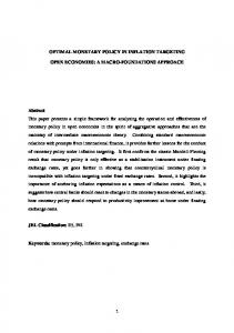
Figure 1 plot two output gap measures obtained from the Hodrick-Prescott filter and smoother with λ equal 1600 using quarterly data for Malaysia from 1991(1) to 2006(4). The HP application acts as a smoother of real GDP that is known as a trend component for potential output, and as a true filter at the end of the sample as a cyclical component that for output gap. These two different concepts, the output gap resulting from the filter is consistent with the policy maker’s interpretation of the cyclical component of real output and provides better out-of-sample forecasts of inflation. The output gap resulting from the filter is negative up to 2000, and ambiguous thereafter, while the output gap resulting from the smoother is positive for the whole period. The filter’s measure of the output gap is more variable than that from the smoother. Given the differences between the properties of the output gap resulting from the smoother and that from the filter, it should be concerned about the economic interpretation of these output gaps. If the policy maker is interested in the current output gap, then the smoother conveys misleading information

about the output gap. However, it is shown that the filter or cyclical output outperforms the smoother or trend output by producing better out-of-sample inflation forecasts from Malaysia sample. Below are the results of the two-stage least square (2SLS) test. Table 1 shows the results of the aggregate supply by using the 2SLS method. The pressure on domestic inflation from output gap is well identified. To ensure that domestic inflation converges to the foreign inflation rate in the long run, therefore a homogeneity condition has been imposed. However, the restriction is not rejected for Malaysia for its coefficient is at 0.881482 and p-value 0.2137. Similarly, it finds no link between real exchange rate and domestic inflation. Nevertheless, the result shows that output gap or capacity utilization is statistically significantly correlated with the domestic inflation at 5% critical value (pvalue is 0.0245) in the long run which is 7.682916 coefficient value. This means that 1% increase in output gap in previous year would increase the domestic inflation in the current year at 7.682916%. Indeed, there is no satisfying converge between the variables, but the link between the variables is positively correlated.

LogReal GrossDomesticProduct

11.2 11.0 10.8 10.6

.10

10.4 .05

10.2 10.0

.00

-.05

-.10 1992

1994

1996

LGDP

Source: Data calculation.

1998

2000

Trend

Figure 1: Hodrick-Prescott Filter Application.

2002

2004

Cycle

2006

Year

196

Table 1: Aggregate Supply Result

Variable Coefficient t-statistic Probability C 0.072627 0.057523 0.9545 Output Gap(-1) 7.682916 2.361546 0.0245** Foreign Inflation(-1) 0.881482 1.268684 0.2137 PPP(-1) -0.179483 -0.153093 0.8793 Note: Entries in *, ** and *** are significant at the 1%, 5% and 10% levels, respectively. Source: Data estimation.

Table 2: Aggregate Demand Result

Variable Coefficient t-statistic Probability C 1.061863 1.546447 0.1346 Output Gap(-3) 0.419190 1.870005 0.0732*** Domestic inflation(-1) -0.005221 -0.406594 0.6878 PPP(-2) -0.043747 -0.434916 0.6674 Government Consumption(-2) -0.108876 -1.196199 0.2428 Three month interbank rate(-1) -0.012209 -2.272204 0.0319** Note: Entries in *, ** and *** are significant at the 1%, 5% and 10% levels, respectively. Source: Data estimation.

Table 2 shows the result of the aggregate demand equation 2. It can be seen from the table that only nominal interest rate and lag 3 output gap are correlated and significant to the output gap in the long run in which the coefficient values are 0.012209 and 0.419190 respectively. This imposes that in the long run the changes in the nominal interest rate would influence output gap which in turn stabilizes the inflation at a lower rate. Nevertheless, other variables are failed to prove correlated with the output gap. For example, government consumption as a proxy of fiscal policy is not significant in influencing the output gap which is similarly with the domestic inflation and real exchange rate that are highly unaffected the output gap. Several aspects of the results discussed in this paper are worth emphasizing. First, output gap has been found to be correlated with the domestic inflation rate. Therefore, domestic inflation rate can be classified as endogenous variable since output gap is statistically significant influence inflation. Otherwise, it fails to prove the opposite relationship between these two variables as can be shown in aggregate de-

mand model. Secondly, foreign inflation is not significant in the aggregate supply model. Therefore, the change in domestic inflation is not influenced by the foreign disturbances. Similarly, purchasing power parity is also not important in influencing domestic inflation rate in the model. However, in aggregate demand model nominal interest rate and real exchange rate have been proved to have a significance relationship with output gap, otherwise for the other variables. This shows that fiscal policy is not important in influencing the ratio of output gap in forecasting the domestic inflation rate. Indeed, it is essential for policy makers to maintain the interest rate at certain level in order to achieve a target of low inflation rate. Besides, the changes of foreign price index and domestic price index are important in influencing the change in the output gap by the real exchange rate

CONCLUSION

The paper suggested that the monetary policy applied in Malaysia only consider the output gap to influence the level of domestic inflation rate which otherwise are not important in transmission mechanism of

The Relationship between … (Antoni)

monetary policy in AS model. The results also indicate that there is a clear tradeoff between inflation and the real exchange rate and that flexibility encourages the adoption of different policies in response to different shocks. When one considers these, the results show that monetary policy under an inflation targeting arrangement may be flexible enough to allow the exchange rate to be addressed on the basis of responding to particular shocks. This is important when one considers the degree to which the infla-

REFERENCES

197

tion targeting central banks in Asia appear to manage movements in their exchange rates. Ultimately, this paper has proved the importance of output gap in predicting or achieving the domestic inflation rate which is controlled by instrumental variable such as interest rate as intermediate target. Therefore, inflation targeting in this case can be categorized as central bank’s inflation forecast by setting the instrument in order to achieve the ultimate goal.

Batini, N., R. Harrison and S. Millard (2003), “Monetary Policy Rules for Open Economies,” Journal of Economic Dynamics and Control, 27(11–12), 2059–2094. Corbo, V., M.O. Landerrretche and K. Schmidt-Hebbel (2001), “Assessing Inflation Targeting after a Decade of World Experience,” mimeo, Central Bank of Chile, Santiago. Debelle, G. and S. Fischer (1994), "How Independent Should a Central Bank be?" Working Papers in Applied Economic Theory No. 94-05, Federal Reserve Bank of San Francisco. Epstein, G. (2006), “Employment Targeting Central Bank Policy in South Africa,” Paper Presented at the Alternatives to Inflation Targeting Monetary Policy for Stable and Egalitarian Growth in Developing Countries conference, Centro de Estudios de Estado Y Sociedad (CEDES), Buenos Aires. Friedman, M. (1968), “The Role of Monetary Policy,” American Economic Review, 18(1), 115-136. Gerlach, S. and M.S. Yiu( 2004), “Estimating Output Gaps in Asia: A Cross-Country Study,” Journal of the Japanese and International Economies, 18(1), 115-136. Golinelli, R. and R. Rovelli (2005), “Monetary Policy Transmission, Interest Rate Rules and Inflation Targeting in Three Transition Countries,” Journal of Banking and Finance, 29(1), 183-201. Granville, B. and S. Mallick (2006), “Does Inflation or Currency Depreciation Drive Monetary Policy in Russia?” Research in International Business and Finance, 20(2), 163-179. Guender, A.V. (2003), “Optimal Monetary Policy under Inflation Targeting Based on an Instrument Rule,” Economics Letters, 78(1), 55-58. Haldane, A.G. (1998), “On Inflation-Targeting in the United Kingdom,” Scottish Journal of Political Economy, 45(1), 1-32. Haldane, A.G. and N. Batini (1998), “Forward-looking Rules for Monetary Policy,” NBER Working Papers, 6543.

198

Harvey, A.C. and S.W. Lewis (1986), “Stochastic Trends in Dynamic Regression Models: an Application to the Employment-Output Equation,” Economic Journal, 96(384), 975-986. Hodrick, R.J. and E.C. Prescott, (1997), “Postwar US business cycles: An Empirical investigation,” Journal of Money, Credit, Banking, 29(1), 1-16. Hsiao, C., (1997a), “Statistical Properties of the Two-Stage Least Squares Estimator under Cointegration,” Review of Economics and Statistics, 64(3), 385-398. Hsiao, C., (1997b), “Cointegration and Dynamic Simultaneous Equation Model,” Econometrica, 65(3), 647-670. IMF, International Financial Statistics, Monthly Report from 1990 to 2004. Mendez, G. and D.R. Palenzuela, (2003), “Assessment Criteria for Output Gap Estimates,” Economic Modelling, 20(3), 529-562. Mise, E., T.H. Kim and P. Newbold (2005), “On suboptimality of the Hodrick-Prescott Filter at Time Series Endpoints,” Journal of Macroeconomics, 27(1), 53-67. Mishkin, F.S., (1992), “Is the Fisher Effect for Real?: A Reexamination of the Relationship between Inflation and Interest Rates,” Journal of Monetary Economics, 30(2), 195215 Razzak, W. (1997), “The Hodrick-Prescott Technique: A Smoother versus a Filter: An Application to New Zealand GDP,” Economics Letters, 57(2), 163-168. Rudebusch, G. and L.E.O. Svensson, (2002), “Eurosystem Monetary Targeting: Lessons from U.S. Data,” European Economic Review, 46(3), 417-442. Svensson, L.E.O. (2000), “Open-economy Inflation Targeting,” Journal of International Economics, 50(1), 155-183. Svensson, L.E.O. (1998), “Inflation Forecast Targeting: Implementing and Monitoring Inflation Targets,” European Economic Review, 41(6), 1111-1146. Svensson, L.E.O. (1999), “Inflation Targeting as a Monetary Policy Rule,” Journal of Monetary Economics, 43(3), 607-654. Svensson, L.E.O. (2002), “Inflation Targeting: Should It be Modeled As an Instrument Rule or a Targeting Rule?” European Economic Review, 46(5), 771-780. Taylor, J.B. (1993), “Discreation versus Policy Rules in Practice,” Carnegie-Rochester Conference Series on Public Policy, 195-214. Wesche, K. A., and S. Gerlach (2008), ”Money Growth, Output Gaps and Inflation at Low and High Frequency: Spectral Estimates for Switzerland,” Journal of Economic Dynamics and Control, 32(2), 411-435.