Monitoring and mining GPS traces in transit space* Leon Stenneth1, 2, Philip S. Yu2 Nokia L&C, Chicago, Illinois, USA 2 Department of Computer Science University of Illinois, Chicago, USA
1
[email protected],
[email protected] Abstract Users of mass transit systems such as those of buses and trains normally rely on accurate route maps, stop locations, and service schedules when traveling. If the route map, service schedule, or stop location has errors it can reduce the transit agency’s ridership. In this paper, the problem of deriving transit systems by mining raw GPS data is studied. Specifically, we propose and evaluate novel classification features with spatial and temporal clustering techniques that derive bus stop locations, route geometries, and service schedules from GPS data. Subsequently, manual and expensive field visits to record and annotate the initial or updated route geometries, transit stop locations, or service schedules is no longer required by transit agencies. This facilitates a massive reduction in cost for transit agencies. The effectiveness of the proposed algorithms is validated on the third largest public transit system in the United States. General terms Algorithms, Design, Experimentation, Performance Keywords Classification, clustering, GPS tracking, maps, mobile, probe
1. Introduction One goal of transit agencies is to increase the ridership of its transits. A strategy for transit agencies to increase their ridership is to improve the user experience of the commuters who utilize these transit systems. A way of improving the user experience has taken the form of intelligent transportation systems (ITS), where spatial and temporal information such as route geometries, stop locations, real time bus locations, and service schedules are correct and accessible via the Internet. For example, see [5]. There is a high cost associated with these intelligent transportation systems. Commercial ITS providers such as NextBus [1] and Clever Device [3] are the predominant venders. However, usage of these services incurs extensive initial and recurring fees. One transit agency budgeted over $20M USD for implementation of such intelligent transportation systems [2]. Transit agencies in emerging markets or developing countries may not have such substantial transportation budgets. Hence, they cannot provide these basic services to the riders of their transits. Often, transit systems have predetermined knowledge of their transit artifacts such as bus stop locations, schedules, and route geometries (i.e. actual current transit path on maps). The problem for these agencies is maintaining updated artifacts, since artifacts can change due to re-routes, weather, construction, event etc. In this paper, novel technology is presented that automatically derives and updates transit systems from the raw GPS traces of the transits. In other words, using these newly proposed algorithms, transit agencies can derive or update their own transportation systems. This automated strategy to derive a transit system from raw GPS traces reduces cost to the transit agency. __________________________________________________ *This work is supported in part by Nokia L&C, NSF through grants IIS0905215, CNS-1115234, IIS-0914934, DBI-0960443, OISE-1129076, and Huawei grant.
In this work, we use the terms transits and buses interchangeably. This proposed work first tracks the moving objects (i.e. buses) for a period of time. During the tracking phase, the locations and timestamps of the buses are recorded. The location of the buses can be determined by a location enabled smartphone [2] or from an onboard GPS device in the bus. Given the location and timestamp data obtained from the location tracking phase, the transit artifacts consisting of bus stop locations, route geometries, and timetable schedule is derived automatically, using spatial and temporal mining on the collected GPS data. Using data mining technology, we propose three algorithms that can extract transit systems from raw GPS traces [2, 26, 27, 28]. The first is a supervised learning bus stop detection algorithm. The second is a spatial clustering route derivation algorithm. Finally, a temporal clustering scheme that produces a service schedule is proposed. For bus stop detection, there is first a route aggregation phase where GPS data from the same transit route are processed together. With this aggregated route based data, a supervised learning technique that captures the mobility pattern of the probes using a density distribution histogram is considered for automated bus stop detection. This strategy first forms cluster points using a spatial constraint scheme. After this spatial constraining step, the results are then utilized in a subsequent aggregation step, which considers a new spatial requirement. This new spatial requirement enables pattern mining on the residuals, and also acts as a constraint on the distance between the predicted and the true bus stop location. Residuals are clusters associated with the initial spatial constraint. Finally, a density distribution histogram that captures the distribution of the residuals within the latter aggregation is constructed. The 10 normalized bins of the histogram and three other mobility patterns become supervised learning classification features for bus stop detection. For route derivation, a simple yet effective six step spatial clustering algorithm is proposed. This algorithm coalesces the different GPS traces from different buses into a single line string (i.e. successive latitude and longitude pairs) representing the route. Spatial outliers that result from GPS inaccuracies are suppressed and pruned, while the remaining points are used to construct the route. The algorithm operates on historical probe archives or real time probe data streams using a spatial and temporal ordering strategy. For service schedule extraction, the temporal property of the GPS data is mined using a K-means temporal clustering scheme. This scheme computes and utilizes the number of trips for a given bus stop as the K value in K-means. In summary, the research and scientific contributions of this manuscript are as follows.
A supervised learning algorithm for automatically deriving bus stop locations from the collected GPS data.
This algorithm requires no driver interaction or user input. A six stage spatial clustering algorithm that automatically derives the set of service routes and the geometries that represent them. A temporal clustering strategy that generates a given transit agency’s service schedule for each bus stop. An evaluation of the proposed algorithms on the third largest transit system in the USA. Namely, the Chicago Transit Authority (CTA) [4].
The remainder of the paper is organized as follows. Next, we highlight other motivations and challenges. Section 3 deliberates the definitions and model, while the supervised learning bus stop detection strategy and its evaluation are presented in Sections 4 and 5. Section 6 addresses transit route derivation and Section 7 discusses service schedule derivation. The related work and conclusion are in Sections 8 and 9 respectively.
2. Motivation and challenges In this section, the motivation for the research is presented. Additionally, the challenges are highlighted and discussed. In this work, the minimum requirement for a real time transit tracking system is an in-vehicle location tracking device. This invehicle device, sometimes referred to as an Automatic Vehicle Locator (AVL), uses GPS or other localization systems to determine the bus’s current location. The location information is then transmitted over a wireless link to the back office. The back office component is a server that processes the incoming location traces, and typically provides a live tracking website for the public and status monitoring for the transit agency’s dispatchers. Several motivations for this work exist. Transits agencies find it costly to derive and update the transit artifacts (route geometries, stop location, service schedules) of their service areas [1, 2]. These transit artifacts are not static, for example bus stops can be added or removed from a transit route for several reasons, such as, extreme weather or construction. Likewise, the geometry of a route may change due to bus re-routes. Thus, these transit artifacts must be kept updated in order for the correct information to be presented on the map. Using these proposed algorithms, we can derive the updated location of bus stops automatically by tracking the transits and then mining the spatial and temporal data obtained from the tracking phase. Additionally, the historical route geometry and updated deviations from the historical routes can be derived. Thus, the issue of transit agencies paying companies such as NextBus [1] or Clever Devices [3] millions of dollars to derive and monitor the transit network can be avoided. Instead, the transit agency can utilize the proposed algorithms. One transit agency with a budget of over USD $250M paid USD $24M for intelligent transportation services that monitors their transit system [2, 4]. Yet, they still cannot recreate routes on demand or automatically detect addition or removal of bus stops. This work targets these updating problems in mature transit systems. Additionally, the proposed solutions are effective for emerging smaller transit agencies to derive their initial transit information systems. Several challenges exist in this research. These include for example: Localization via GPS can be inaccurate; hence the location that the buses report may not be the true location. Each bus on the same route will report completely different location points.
Buses deviate from their true routes at times. For example, a bus may detour because of an accident. Buses submit GPS reports every 20-30 seconds. Generally, the reports are sparse. Thus, a bus may service a bus stop quickly without submitting a GPS report while at the bus stop. The data model is limited since we consider the minimum requirement which is location and timestamp.
3. Definitions and model In this section, the definitions, model, and architecture are discussed. Definition 1 – Probe – We define a probe P to be a vector of the form (sys_id, route_id, bus_id, locgps). Where sys_id is the identification of the transit agency (e.g. CTA or San Francisco’s BART), route_id is the route that the corresponding bus services, bus_id is the identification number of the bus, and locgps is the location property of the bus. In this work, in order to validate the algorithms we consider the third largest transit network in the United States; this is the Chicago Transit Authority (CTA). In this system, probes are submitted by each bus every 20-30 seconds. Definition 2 - GPS report – We define a GPS report locgps to be a vector of the form (lat, lon, time) where lat is the bus’s latitude and lon and time is the longitude and timestamp of the report respectively. Definition 3 - GPS trace – For a given bus bi, a GPS trace is a temporally ordered sequence of GPS reports submitted by bi. Given n buses b1, b2, b3… bn, where each active bus bi submits a probe at time t. Thus, over time, for each bus bi we have a list of probes where is the last probe submitted by bi. Each probe has a GPS report and from the list of probes we can get a GPS trace for the bus bi. The probes that are submitted by the buses become the input for the algorithms. In order to evaluate the algorithms, we utilize over 10,000,000 probes. From the probes, we will use newly proposed supervised and unsupervised data mining techniques to extract the location of bus stops, route geometries, and service schedule. Assumption: We assume that buses may stop periodically at the start or end of trips.
3.1 Architecture and data flow The architecture is depicted in Figure 1. As illustrated in Figure 1, the buses possess a tracking component that periodically transmits its location data to the location server. This data can be transmitted over a cellular link. The in-vehicle location device may be permanently installed in the bus (e.g. on-board GPS) or carried by the driver (e.g. smartphone with localization capabilities). The traces from the buses are then archived. Using the route aggregator, probes from the same routes are aggregated and then processed. After the route aggregation phase, the proposed supervised learning algorithm is then activated for bus stop extraction. Likewise, the spatial clustering route extraction and the temporal clustering schedule extraction algorithms are also activated. The derived bus stop locations, route geometries, and service schedules are called transit artifacts and are archived for use in the transit agency’s information system. Once the transit artifacts are
derived, the buses’ spatial and temporal properties are then monitored for deviations. When deviation occurs, alerts are activated in the system. For example, using transit artifacts we are aware of the route geometry and bus stop locations. If buses deviate from the historical route geometry in the transit artifact, then a re-route alert is activated. We can also generate bus stop removal/addition alerts in real time. Further, if buses deviate from their historical scheduled time, we generate temporal based alerts such as bus delayed or running ahead of schedule.
Figure 1- architecture overview
4. General algorithm for bus stop detection In this work, stop extraction is the process of turning a set of raw GPS traces belonging to a given route into a small set of coordinates; indicating the locations of transit stops. The locations generated by the proposed algorithm are used for producing arrival times for schedule extraction or for drawing stop locations on a route map, this allows travelers to be aware of boarding locations. Here, we define the concept of a mini-cluster. Definition 4: mini-cluster – In this work, a mini-cluster is a cluster formed with probe points that are a spatial requirement of 3m from each other. In this work, 3m is the distance selected, empirically, to balance between sufficient data density and reasonable run time. However, one can tune this spatial requirement and observe the bus stop detection accuracy of the machine learning model before system deployment. The cluster algorithm is purely spatial, and a cluster’s center continues to shift when a new GPS point is added to a cluster. A GPS point can only exist in a single mini-cluster. In general each cluster has a center which is the weighted average of all the points within that cluster. Definition 5 - cmax - We define cmax to be a value corresponding to the size of the densest mini-cluster along the route. Thus, cmax varies per route and across routes. Based on experiments, we found that cmax is at the start or the end of routes. The maximum cluster size is obtained by comparing the number of GPS reports within each mini-cluster along the entire route. Mini-clusters provide information that can be used to distinguish a bus stop from other points. At bus stops, we expect a few mini clusters with high densities. For a stop light along a route, the distribution of the mini-clusters is sparser and density of mini-clusters is lower than at bus stops. Given these mini-clusters, we then form cluster sets which are 20m bounding boxes along a route that contains several mini-clusters. Thus, bus stop detection is approximately within 20m from the true bus stop location.
Definition 6 – cluster set – a cluster set is a square bounding box with coordinates (x, x’, y, y’). In this work, x’-x =20m and y`-y =20m. The value of 20m was chosen empirically and ensures that when the algorithm predicts a bus stop location it is reasonably close to the true bus stop location at most 20m away. One can tune this spatial requirement. The intuition behind this step of mini-clusters being overlaid by cluster sets is that for bus stops, buses always stop close to the bus stop for passengers to board/alight. Consequently, at a bus stop the number of GPS reports should be high (i.e. dense miniclusters). For other points on the route, since the buses are not stopping the number of GPS reports should not be as high as at a bus stop. On the other hand, regions around stop lights and stop signs may also observe a high frequency of reports. However, these objects (stop lights and stop signs) have different distribution patterns which we can use to identify and distinguish between them and bus stops. For one example, at stop signs buses hardly ever stop completely, for a long time. We observe that they (i.e. buses) mostly slow down or stop briefly. For another example, in the case of stop lights, buses stop at arbitrary points when adhering to any given stop light. In other words, for a given stop light, a bus maybe adhering and stops at 400m (e.g. in traffic), 40m, 50m, or 5m from the stop light. This is not the case for bus stops, instead, drivers tend to stop their buses as close as possible to the bus stop because of their business. Using spatial pattern recognition principles, machine learning models are then trained to automatically recognize and identify these mobility patterns. The mobility patterns for classification are then mined from the cluster sets along the route. These mobility patterns capture the mini-cluster density and distribution within the cluster sets using 13 newly proposed classification features. Ten of the 13 classification features are bins of the histogram that represent the density distribution of the mini-clusters within a cluster set. The other 3 features are related to other mobility patterns. With these 13 classification features, multiple supervised machine learning models (e.g. Bayes Net, Random Forest, and Decision Trees) are trained. Then, when bus stop location is to be determined, the unlabeled data is used to create the same features that were used for training. These features are then fed to the machine learning model that is already trained. This trained model can then determine, in a probabilistic format, the presence of a bus stop. Given this trained supervised machine learning model, we can then utilize it on any transit system to discover or update bus stop locations.
4.1 Parameter tuning In this work, the spatial requirements for mini-cluster and cluster set were chosen empirically. Realistically, one should tune these parameters while observing the accuracy of the supervised learning scheme in order to deduce the optimal spatial parameter settings.
4.2 Generate distribution histograms A histogram for each cluster set layered along the route (See Figure 2) is generated. In Figure 2, the boxes represent the cluster set and within each cluster set are the mini-clusters. A distribution histogram is then generated for each cluster set. This histogram captures the distribution of the GPS reports within each minicluster in the cluster set. The histogram contains 10 bins. Each bin of the histogram is a fraction of the maximum cluster size cmax.
4.5 Machine learning component In this section, we present the machine learning model, dataset, and the machine learning algorithms that we considered for evaluation.
4.5.1 Training model Figure 2- Generate histogram for each cluster set More specifically, each bin of the histogram except the last bin contains 5% increment in terms of fraction of cmax. Thus, the first bin contains the number of mini-clusters in the cluster set with number of reports