Publishers, Amsterdam. [16] Peter Folger(2011) Earthquakes: Risk, Detection,. Warning, and Research. Congressional Research Service. 7-5700 www.crs.gov.
International Journal of Applied Information Systems (IJAIS) – ISSN : 2249-0868 Foundation of Computer Science FCS, New York, USA Volume 4– No.3, September 2012 – www.ijais.org
Monitoring and Prediction of Earthquakes using Simulated Temperature Deviation Curve Model Moses E. Emetere Department of Physics, Federal University of Technology of Minna
ABSTRACT The use of thermal anomaly to monitor or predict earthquakes has shown little success. Various methods have been propounded to monitor earthquakes with little emphasis on fundamental soil quantities. This paper propounded a vital factor- soil density ratio which can be used to monitor earthquakes. The magnitude of earthquakes was discovered to increase when the soil bulk density decreases very low. The dynamics of the heat flow was also discussed with respect to the soil density ratio. The importance of the temperature deviation curve to predict both short term and long term earthquakes were discussed with respect to time.
Keywords soil density ratio, temperature deviation, heat frequency, earthquake duration, earthquake magnitude
1. INTRODUCTION Soil temperature is an important factor in predicting soil chemical reactions, solute transport, gas exchange and transport of contaminant (Buchan,2001).The solution of water movement through earth structure using flow net technique(Casagrande,1937)was discovered (Nguyen,1999) to play an important role in geothermal structure of the earth. The existence of the geothermal structure of the earth has been explained severally with respect to soil temperature. Therefore thermal properties of soil are vital because its changes suggest a possible existence of interaction between the lithosphere and the atmosphere in seismic zones prior to the occurrence of earthquakes (Dey et al. 2003) For example, Fan et al. (1996) related the occurrence of earthquakes to a peculiar kind of soil temperature distribution in the Mongolia, Bohai, Chongqing and Xingtai regions of China. Likewise Rezapour et al. (2010) related the ground temperature with the earthquake in Alborz region of Iran. It was reported (Rezapour et al.,2010) that the positive soil temperature anomaly dominated the region or area several months before the earthquake occurrence, and the positive anomaly area enlarges gradually and its intensity also enhances simultaneously. When the earthquake occurs, the positive anomaly area reaches its maximum and the intensity remains the same. The idea of seismogenic soil temperature field was therefore regarded as the shallow layer soil temperature fields around strong earthquakes (whose magnitude is above seven). Fan et al.,(1996) conducted a research on the soil temperature data of three layers of soil depth 0.8 m. 1.6 m, and 3.2 m. The results was used to calculate the shallow layer soil heat flux and changes of shallow layer soil heat flux during the seismogenic period of strong earthquakes. Beyond using soil temperature distribution to predict earthquakes, other parameters have been used, for example, geophysical and
ionospheric parameters was used by Uyeda et al., (2000); meteorological parameters was used by Rezapour et al.(2010); satellite based analysis was used by Qiang (2001);seismoionosphere coupling was used by Gokhberg et al(1995) and Parrot et al(1993); ionosphere precursor of earthquake was used by Pulinets(2004) to predict short time earthquakes; state of the art-elevation maps used by the Department of Geology and Minerals Industrial Mcconnell (2012). Presently, the mapping of Oregon has been interpreted as likely to face earthquake of magnitude 9.0 because Oregon and Japan sit on the same subduction zones where the ocean floor is slowly thrust beneath the land (Mcconnell 2012). Earthquakes have been observed to occur at time intervals within an earthquake prone area(Mcconnell, 2012; Forlger (2011) . For example Alaska in United State of America(U.S.A) experiences a magnitude 7.0 earthquake every year and magnitude 8.0 at every fourteen (14) years on the average(Forlger, 2011). The temperature deviation curve model has shown successes (Uno et al., 2012a;2012b) which includes: determining the susceptibility of Abuja metropolis to soil compaction; calculating the annual amplitude of the surface soil temperatures; analysis of soil heat flux of regions within Abuja and Niger of Nigeria. The importance of the temperature deviation curve model is a simulation programme which is less expensive to be used by research institute in developing countries. This paper demonstrates the use of temperature deviation curve model to predict disaster prone regions through the use of temperatures deviations from its mean soil temperatures over a hypothetical region. Some of the parameters used in this paper where adopted from practical results of Fan et al. (1996) and Rezapour et al.,2010. .
2. MATHEMATICAL FORMUATIONS Fan et al.,(1996) introduces the analytical solution of one dimensional thermal conductive equation as ( (
)
[ ( )√
)
)√ ]
( [1]
Where A is amplitude, ω is circular frequency, β is initial phase, T(z,t) is the soil temperature at time (t), z is the soil depth, Ta is the average soil temperature (oC), A0 is the annual amplitude of the surface soil temperature (oC), d is the damping depth (m). [2] The volume thermal capacity was given as Cw = pc = 1.256 J.cm"-K" by Tang et al. (1990). p is medium density, c is specific heat, a is constant, = soil heat flux, = thermal diffusivity
13
International Journal of Applied Information Systems (IJAIS) – ISSN : 2249-0868 Foundation of Computer Science FCS, New York, USA Volume 4– No.3, September 2012 – www.ijais.org The temperature deviation curve model introduced by Unoh et al.,(2012a) is given by
When
the temperature deviation model becomes (
⁄
(
)
)
[6]
[3] [7] -3
= soil particle density which is a approximately 2.66gcm by Gupta et al.,. (2011), = soil bulk density. ΔT= temperature deviation, A0 is the annual amplitude of the surface soil temperature. At resonance ( , a=0),when the phase angles of equation[1] and [3] are the same, equation [4],[5] are generated
(
) ( )
[8]
K is the hydraulic conductivity. Where M is the magnitude of the earthquake
3. SIMULATIONS OF DERIVATIONS
[4]
[5]
t
t
b
a
ω
ω t
t
c
d
ω
ω
Fig1(A-D):Analysis Of The Time When Frequency Varies From 0.015Hertz To 1500Hertz. Figure 1a Was Analyzed When The Frequency Is 0.015Hertz. Figure 1b Was Analyzed When The Frequency Is 1.5Hertz. Figure 1c Was Analyzed When The Frequency Is 150Hertz. Figure 1d Was Analyzed When The Frequency Is 1500Hertz.
T
T
T
T
Figure 2(A-D): The Relationship Between The Temperature(T) And Heat Flux Density(Qd) As The Time Increases Within The Range Of 1hour To One Year. Fig 2a Was Analysed At One Hour. Fig 2b Was Analysed At One Month. Fig 2c Was Analysed At One Hour Six Month. Fig 2d Was Analysed At One Year.
14
International Journal of Applied Information Systems (IJAIS) – ISSN : 2249-0868 Foundation of Computer Science FCS, New York, USA Volume 4– No.3, September 2012 – www.ijais.org
ΔT
ΔT
ΔT
ΔT
Figure 3: The Deviation The Soil Temperature From Normal During Earthquakes. The Soil Heat Flux And Duration Remains The Same As In Figure 2.
T
Figure 4: Relationships between Soil Temperature Deviations And Soil Density Ratio ( ) Moments Before The Earthquake. Red Line Indicates One Hour, Blue Line Indicates One Month, Green Line Indicates Six Months And Purple Line Indicates One Year.
T
Figure 5: The Temperature Deviation Curve At Different Phase At Durations Ranging From 1hour To One Year. Red Line Indicates One Hour, Blue Line Indicates One Month, Green Line Indicates Six Months And Purple Line Indicates One Year.
15
International Journal of Applied Information Systems (IJAIS) – ISSN : 2249-0868 Foundation of Computer Science FCS, New York, USA Volume 4– No.3, September 2012 – www.ijais.org
Figure 6:The Relationship Between The Magnitude Of Earthquake Soil Density Ratios When The Hydraulic Conductivity Is Less Than Ten. Figure 6a Is When The Frequency Is 0.015Hertz. Figure 6b Is When Frequency Is 1.5Hertz. Figure 6c Is When The Frequency Is 150Hertz. Figure 6d Is When Frequency Is 1500Hz. In All The Figures, The Soil Density Ratios ( ) Is Between 0 And 500.
Figure 7: The Relationship Between The Earthquake Magnitude And The Soil Density Ratio When It Ranges From 0 To 1000.
4. RESULTS AND DISCUSSION Figure 1(a-d) showed a linear relationship between the period of earthquake and the frequency. From the graph, the phase difference between the period of earthquake and the frequency was calculated to be ≤ . The phase differences increases as frequency increases. The soil temperature and the soil heat flux were found to exhibit special features (Figure 2). No negative values for both quantities were obtained which corresponds to Rezapour et al. (2010) discovery of positive soil temperature which he claimed to be a possible trace of natural disaster. Also, the relationship between the soil temperature and the soil heat flux is parabolic. This simply means that the computation of quantities expresses an exponential value which may likely vary from region to region of the globe. The deviation between the normal from its mean temperature (Figure3) indicates that it decreases as the period of earth elongates while its soil heat flux increases within the same period. The lowest value of the soil density
ratio was at about 7(Figure 4). Beyond minimum point (i.e. 7), the soil density ratio starts increasing with respect to the increase of soil temperature. This suggest that heat flow is enhanced when which leads to other occurrences before earthquakes. The possibility of was investigated. A sinusoidal graph was obtained between the temperature deviation and phase difference. The amplitude of equation (6) decreases as the time increases (see figure5) Also, compared with the graphs displayed by Mcconnel(2012), Figure 5 represents series of waves(tsunami) with respect to the temperature increase and the yellow ring represents area of likely earthquake occurence. The relationship between the magnitude of an earthquake and the soil density ratio was investigated in figure 6 and 7. Increase of frequency has reduced or insignificant impact to the magnitude of the earthquakes. However, the soil density ratio reveals that natural disasters e.g earthquake may occur in within a region .
16
International Journal of Applied Information Systems (IJAIS) – ISSN : 2249-0868 Foundation of Computer Science FCS, New York, USA Volume 4– No.3, September 2012 – www.ijais.org
5. CONCLUSION The anomaly in the soil heat flux has been found to be a vital factor for monitoring earthquakes and health hazard on the globe. The sharp anomaly in the soil density ratio is an indication of tremors or earthquake in a region. Places around the globe whose soil bulk densities decreases drastically experienced earthquakes of three and above (≥3). Therefore a earthquake of ≥8, the density ratio (
) would be ≥1500.
6. APPRECIATION This work is self-funded. I appreciate Mrs. Jennifer Emetere for editing the script. I appreciate the Head of Physics Department of the above named institution
7. REFERENCE [1] Buchan, G.D.,2001.Soil Temperature Regime, in Smith, K.A and Mullins, C.E.(Eds). Soil and Environmental Analysis: Physical methods 2nd Ed.2001. Marcel Dekker. Pp, 539-594 [2] Hillel, D. 1982. Introduction to soil physics. Academic Press, San Diego, CA. [3] Uno E Uno, Moses E Emetere, Adelabu J.S.A. 2012. Parametric Investigation Of Soil Susceptibility To Compaction Using Temperature Deviation Curves. Journal of Civil Engineering and Architecture Vol. 2012,issue 2 pp.1-6 [4] Fan Xin-gang and Tang Maocang.1996. The Structural Features of Soil Temperature and Precipitation and Soil Heat Flux Fields of Strong Earthquakes. Chinese Journal of Geophysics 39/2 247-260. [5] Uno E Uno, Moses E Emetere, Eneh C Daniel.2012. Simulated Analysis Of Soil Heat Flux Using Temperature Deviation Curve Model. Science Journal of Physics. Vol. 2012, Issue 2,pp 1-9 [6] Uyeda, S., Nagao, T., Orihara, Y., Yamaguchi, T., and Takahashi,I. 2000. Geoelectric potential changes:
Possible precursors to earthquakes in Japan, Proc. Nat. Acad. Sci., 97, 4561–4566 [7] Rezapour N., Fattahi, M. and Bidokhti A. A. 2010.Possible soil thermal response to seismic activities in Alborz region (Iran) Nat. Hazards Earth Syst. Sci., 10, 459–464, [8] Casagrande, A. 1937. Seepage through Dams. J. New England Water Works. 51 295-336 [9] Dey, S. and Singh, R. P.2003 Surface latent heat flux as an earthquake precursor. Nat. Hazards Earth Syst. Sci., 3, 749–755 [10] Nguyen, T.M.T.1999. Solution of saturated/unsaturated seepage problems using a general partial differential solver. M.Sc. Thesis, University of Saskatchewan, Saskatoon, Canada [11] Qiang, Zuji, 2001. Satellite-Based Prediction Earthquakes. News letter, EARSEL 47, 21-26
of
[12] Tang Maocang and Hu Zong-hai(1990) Statistical analysis of strong earthquake influencing precipitation, Nonhwestem Seismological Journal (in Chinese), 12 (I), 19-29 [13] Vicki S. McConnell (2012) Oregon Department of geology and mineral industries Magazene. www.oregongeology.com [14] Sergey Pulinets(2004) Ionospheric Precursors of Earthquakes; Recent Advances in Theory and Practical Applications. TAO, Vol. 15, No. 3, 413-435 [15] Gokhberg, M. B., V. A. Morgounov, and O. A. Pokhotelov, 1995: Earthquake Prediction.Seismoelectromagnetic phenomena. Gordon and Breach Science Publishers, Amsterdam. [16] Peter Folger(2011) Earthquakes: Risk, Detection, Warning, and Research. Congressional Research Service 7-5700 www.crs.gov
17