ferred to as hot spots (Levine, 1996; Liu, Dong. & Chi, 2010). ..... zi is the deviation of an attribute for feature ifrom its mean; wi j, is the spatial weight between features i and j ..... ics, 63(2), 385â404. doi:10.1016/j.jue.2007.12.002. Environmental ...
International Journal of Applied Geospatial Research, 5(3), 1-20, July-September 2014 1
Monitoring Urban Sprawl and Sustainable Urban Development Using the Moran Index:
A Case Study of Stellenbosch, South Africa Walter Musakwa, Department of Geography and Environmental Studies, Stellenbosch University, Stellenbosch, South Africa Adriaan van Niekerk, Department of Geography and Environmental Studies, Stellenbosch University, Stellenbosch, South Africa
ABSTRACT The management of urban sprawl is fundamental to achieving sustainable urban development. Monitoring urban sprawl is, however, challenging. This study proposes the use of two spatial statistics, namely global Moran and local Moran to indentify statistically significant urban sprawl hot and cold spots. The findings reveal that the Moran indexes are sensitive to the distance band spatial weight matrices employed and that multiple bands should be used when these indexes are used. The authors demonstrate how the indexes can be used in combination with various visualisation methods to support planning decisions. Keywords:
Distance Band, Global Moran I, Local Moran I, Spatial Cluster and Outlier, Sustainable Urban Development, Urban Sprawl
INTRODUCTION Urban sprawl is a fundamental theme in the sustainability debate (Zhao et al., 2011) and literature often equates sprawl with unsustainability (Le Néchet, 2012). However, what is unsustainable about urban sprawl are its wasteful forms, so that future generations can be deprived as a result of dwindling resources used to make way for urban expansion (Gerundo & Grimaldi, 2011). If urban growth is to continue it better be sustainable rather than wasteful (Ewing, 1997;
Veneri, 2010). Planners have accordingly adopted the use of geographic information systems (GIS) and earth observation (EO) data to identify wasteful forms of urban sprawl commonly referred to as hot spots (Levine, 1996; Liu, Dong & Chi, 2010). Most GIS packages are able to do this by providing summary statistics such as means, sums and medians. However, such statistics cannot be generalised over various locations making it difficult to compare various urban centres. Moreover, visual representations of such results are also known to be misinter-
DOI: 10.4018/ijagr.2014070101 Copyright © 2014, IGI Global. Copying or distributing in print or electronic forms without written permission of IGI Global is prohibited.
2 International Journal of Applied Geospatial Research, 5(3), 1-20, July-September 2014
preted (Zhang et al., 2008). What is required are new software and exploratory data analysis techniques that focus on the spatial aspects of the data such as dispersion, concentration and spatial autocorrelation which can be used to capture the impacts of urban sprawl on urban sustainability (Anselin, 1995; Le Néchet, 2012). This provides a scientific basis for improved sustainable land use planning. Similar analyses have been successfully carried out for pollution (Zhang et al., 2008), conflict (Anselin, 1995), disease (Ruiz et al, 2004; Zhang & Lin, 2006) and crime management (Anselin et al., 2000; Lin & Brown, 2006). Concerning urban sprawl, a search on Science Direct, Scopus and Web of Science databases1indicate that Tsai (2005) was the first to apply the global Moran index (Moran I) to distinguish urban sprawl from compactness. Similar studies citing Tsai (2005) ensued, such as Gerundo & Grimaldi (2011), Le Néchet (2012), Sim & Mesev (2011), Zhao et al. (2011) which employed global Moran index (Moran I) and other metrics to distinguish between urban sprawl and compactness in European, American and Asian cities. Moran I has attracted interest from researchers and planners because it is apparently more robust than other metrics (Bhatta, Saraswati & Bandyopadhyay, 2010). To the best knowledge of the authors, no studies exist that have applied the global Moran and local Moran indexes with cluster and outlier analysis to cadastral data to determine sprawl hot spots and cold spots. This study investigates the use of these indexes with GIS software and cadastral data to identify urban sprawl hot spots. Moreover, the impact of various simulations (weights) of the indexes is explored and the practical implementation of this process in policy change and decision making toward sustainable urban development is investigated.
URBAN SPRAWL The debate on measuring and monitoring urban sprawl continues unabated (Bhatta, Saraswati & Bandyopadhyay, 2010). However, there is
consensus that urban sprawl is primarily characterised by three attributes, namely leapfrog and scattered development, commercial strip development and large expanses of low-density or single-use development (Frenkel & Ashkenazi, 2008; Sayas, 2006; Sims & Mesev, 2011; Tsai, 2005). Leapfrog development, strip and low-density development do not necessarily equate to unsustainable urban development. Consequently, it is a matter of degree and the impact of the development that make various types of urban sprawl unsustainable (Ewing, 1997; Vaz et al., 2012). For example, a housing development may leapfrog a rock outcrop and have a mix of uses which support non-motorised transport (NMT), promote accessibility, reduce vehicle miles travelled (VMT), and encourage social interaction. Such developments are unlikely to be unsustainable forms of urban sprawl (Le Néchet, 2012). It is the quantifiable and related impacts that make development patterns urban sprawl (Ewing, 1997). The literature identifies poor accessibility as one of the most important indicators of urban sprawl (Cervero, 2002; Irwin & Bockstael, 2007). Accessibility implies that urban development patterns are spatial and that accessibility can be quantified by indicators such as VMT (Le Néchet, 2012). Other urban sprawl indicators include lack of functional open space, visual aesthetics, spatial geometry and densities (Hayek et al., 2011; Schwarz, 2010). Poor accessibility impacts household travel patterns. Recent studies demonstrate that average trip length and travel time which impact greenhouse gas (GHG) emissions increase with the poor accessibility associated with urban sprawl (Urban Land Institute, 2010). For example, in some low-density single-use developments everything is far apart as a consequence of the separation of land uses leading to increased trip lengths (Irwin & Bockstael, 2007). Gore (1993) has observed that a gallon of gasoline can be used just driving to get a gallon of milk. An important urban development problem related to accessibility is lack of functional
Copyright © 2014, IGI Global. Copying or distributing in print or electronic forms without written permission of IGI Global is prohibited.
International Journal of Applied Geospatial Research, 5(3), 1-20, July-September 2014 3
open space. It is difficult to preserve large open spaces in low-density developments where the emphasis is on subdividing every piece of land, leaving little space for community use or the creation of elite social enclaves (Ewing, 1997; Frank & Engelke, 2001). Furthermore, lack of functional open space normally entails deprived visual aesthetic stimulation, reduced biodiversity support and ineffective flood control (Giarrusso, 2003). Residential areas in many cities in developing countries are located far from areas of economic opportunity, and they have little or no functional open spaces and basic services; the result of pre-independence urban planning policies (Western Cape Department of Environmental Affairs and Development Planning, (WCDEADP) 2009). Convalescing such types of planning will perhaps lead to better accessibility and ultimately gains in urban sustainability. Another indicator of urban sprawl is spatial geometry which determines the configuration and composition of the urban landscape (Frenkel & Ashkenazi, 2008). Urban sprawl’s geometric configuration is usually irregular, scattered or fragmented (Sims & Mesev, 2011), whereas composition refers to homogenous land use and segregation of land uses. Measures to classify geometry and composition include leapfrog measures and the land use mix index. Besides spatial geometry, densities are probably the most common and widely studied measures of urban sprawl (Huang, Lu & Sellers, 2007). Density is the ratio between the quantity of an urban activity, for example buildings or population, and the area within which the activity takes place (Angel, 2010; Burton, 2002). In South Africa, very low building densities of less than 30 buildings per hectare signify a sprawling pattern (WCDEADP, 2009). Although the above indicators do denote urban sprawl, they have to be quantified and measured or scaled to determine the impact of urban sprawl on sustainable urban development. Various studies have been undertaken to determine how these indicators impact urban sustainability (Burton, 2002; Urban Land Institute, 2010).
Urban Sprawl and Sustainable Urban Development Urban sprawl is inevitable, especially given the high rate of urbanisation in many developing countries, and it is not necessarily a detrimental phenomenon. It is the inefficient forms and adverse costs of urban sprawl, namely environmental and socio-economic costs, which are deemed unsustainable (Hall, 2010). Environmental costs include increases in VMT, loss of natural resources, increases in energy consumption and air pollution. Socio-economic costs include increases in infrastructure and public services costs, decay in city centres and psychic and social costs which are deemed unsustainable (Ewing, 1997). Concerning the adverse environmental effects of urban sprawl, recent studies have demonstrated the link between VMT and accessibility. Evidence suggests that households in most accessible locations spend 40 minutes less per day travelling than households in least accessible locations (Victoria Transport Policy Institute, 2010). This results in cost savings as well as lower GHG emissions. Furthermore, a study of 34 European cities found that an increase in density implies that trips get shorter while the share of transit and other modes of transport increases (Le Néchet, 2012). Equally important is the impact of urban sprawl on energy consumption because sprawl affects travel patterns and energy consumption in buildings (Canadian Urban Institute, 2008). Findings point out that as people and buildings continue to be spread across urban space, as measured by average distance between two individuals, energy efficiency is reduced (Newman & Kenworthy, 1999). Le Néchet (2012) has concluded that per capita fuel consumption for motor vehicles is much lower in compact cities than in low-density sprawling cities, even though fuel efficiency is less (Bigazzi & Burtini, 2009; Zhao, Lu & de Roo, 2011). There is consensus that vehicle emissions increase with VMT and decrease with average operating speed (Bigazzi & Burtini, 2009).
Copyright © 2014, IGI Global. Copying or distributing in print or electronic forms without written permission of IGI Global is prohibited.
4 International Journal of Applied Geospatial Research, 5(3), 1-20, July-September 2014
These findings confirm that compact development is more sustainable than urban sprawl given the latter’s effect on increasing GHGs which contribute to global warming. Recent studies in Canada report that despite compact and dense developments having a high energy demand2 compared to low-density areas, they allow energy power plants to run at maximum efficiency and they also ensure better return on investment (Canadian Urban Institute, 2008). Notable findings emerged after the USA reduced its GHG emissions by decreasing the carbon content of fuels and through investments that assisted in reducing energy intensity. These include new compact developments and innovative changes to urban planning guidelines (Transportation Research Board, 2009; Urban Land Institute, 2010). The argument that compact development, in contrast to urban sprawl, reduces harmful environmental costs has gained momentum owing to the increased supply of good-quality data and processing tools. There is agreement that compact development, compared to indiscriminate urban sprawl, is the planning practice that best respects people and the environment (Mubareka et al., 2011; Schwarz, 2010). This view challenges Gordon & Richardson’s (1997) contention that urban growth in any form, including low-density and scattered single-use developments is not much different from the supposed sustainability benefits of compact developments. As for infrastructure and service costs, per capita infrastructure costs tend to fall as densities increase but tend to rise in sprawling low-density areas (Glaeser & Kahn, 2004; Song & Zenou, 2006). At very-high densities, these economies of scale diminish so that specific thresholds have to be met, for example limiting densities to 60 buildings per hectare (Urban Land Institute, 2010). Ewing (1997) found that leapfrog developments that bypass suitable land for residential developments raise costs considerably. Other costs which can be incurred include travel and defraying costs to taxpayers. In addition, dense developments provide a steady revenue source that covers
costs of energy infrastructure and amortises the costs (Zhao, 2010, 2011). Urban sprawl not only raises infrastructure costs but also psychic and social costs (Vaz et al., 2012; Wu, 2006). These costs are difficult to measure as they relate to deprivation of access and environmental delight. Deprivation of access is about lack of access to facilities, services and employment for those without cars (Ewing and Cervero, 2001; Stone, 2008). This severely affects the young, the old and the poor. In contrast, environmental deprivation is the absence of elements that provide activity and stimulation (Brown et al., 2009). Studies indicate that urban sprawl’s uniformity deprives residents of interaction compared to compact developments that allow social vibrancy (Eid et al, 2008). This is a characteristic of cities in developing countries such as South Africa (Poulsen, 2010). Urban sprawl also induces loss of natural resources (Angel, 2010). If urban expansion results in rapid losses of flora and fauna, farmland, protected areas and areas of national heritage, they ought to be curtailed as they lead to an impoverishment of resources for future use (Vaz et al., 2012). To minimise loss of resources, planning regulations should be enforced along with raising the awareness of the need for the conservation of natural resources. Finally, urban sprawl can lead to the decline of city centres as new developments favour out-of-town locations (Glaeser & Kahn, 2004; Song & Zenou, 2006). For example, developments north of the Durban central business district (CBD) in South Africa have attracted far more development than central Durban has (EThekwini Municipality, 2007). Similarly, in Harare, Zimbabwe, there has been a flight of capital from the CBD to the north-eastern part of the city, leaving the CBD to invasion by informal businesses (Muronda, 2008). Such developments can lead to inner-city decline as jobs become located farther away and they discourage social and spatial mixing because they promote the creation of social enclaves. In summary, urban sprawl impacts on urban
Copyright © 2014, IGI Global. Copying or distributing in print or electronic forms without written permission of IGI Global is prohibited.
International Journal of Applied Geospatial Research, 5(3), 1-20, July-September 2014 5
sustainability through its wasteful forms which have unfavourable effects for contemporary and future generations (Figure 1). Measuring and monitoring the environmental and the socio-economic costs of urban sprawl is challenging. The advent of EO and GIS tools has provided a range of techniques that could potentially be used for this purpose (Frenkel & Ashkenazi, 2008; Schwarz, 2010). However, most of these techniques capture the negative effects of sprawl visually, but remain uninformative regarding the statistical significance of what they visualise (Zhang & Lin, 2006; Zhang et al., 2008). Moreover, urban planners, particularly in sub-Saharan Africa, have a long history of using exploratory data analysis which ignores the spatial aspects of data despite urban planning and urban sprawl being essentially spatial processes (Mabogunje, 1990; Sayas, 2006). The field of exploratory spatial data analysis (ESDA) which takes into account spatial aspects of data may offer a solution. Anselin (2012) defines ESDA as a “collection
of techniques to describe and visualise spatial distributions, identify atypical locations or outliers, discover patterns of spatial heterogeneity” (p. 137). Urban planners have adopted ESDA and GIS to derive statistics which rigorously quantify spatial relationships (spatial distribution and spatial autocorrelation3) so that conclusions can be drawn which facilitate decision making (Anselin & Getis, 1992).
Indicators of Urban Sprawl Urban sprawl indicators should be able to capture the various adverse effects of the different dimensions of urban sprawl. Urban sprawl indicators should be able to locate urban sprawl hot spots (Sayas, 2006), be statistically significant (Tsai, 2005) and distinguish between a cluster and an outlier (Zhang & Lin, 2006). Several GIS mapping techniques have been used to identify hot spots, but many are not statistically significant making it impossible to distinguish between clusters and outliers
Figure 1. Urban sprawl and its impacts
Copyright © 2014, IGI Global. Copying or distributing in print or electronic forms without written permission of IGI Global is prohibited.
6 International Journal of Applied Geospatial Research, 5(3), 1-20, July-September 2014
(Zhang et al., 2008). The global Moran I and local Moran I indexes have been shown to be more effective in detecting urban sprawl hot spots, clusters and outliers (Table 1) than other indicators such as the Tango index and spatial scan statistics which tend to have a bias toward positive autocorrelation (Zhang & Lin, 2006). Furthermore, global Moran I characterises different aspects of urban sprawl (e.g. density or leapfrogging), which means that separate indexes are not required. This also eliminates the need for synchronisation and weighting of different indexes (Tsai, 2005).
Global Moran I The global Moran I dates from 1948 as a measure of spatial autocorrelation, which quantifies the spatial association between the same variable in neighbouring locations (Moran, 1948). Positive spatial autocorrelation arises when neighbouring areas have similar variable values, while negative spatial autocorrelation occurs when the values of neighbouring areas vary considerably (Anselin, 1995). Global Moran I is expressed as: n I =n So
n
n
i =1
j =1 i , j
∑ ∑
∑
n
w zi z j z i2
(1)
i =1
where z i is the deviation of an attribute for feature i from its mean; wi, j is the spatial weight between features i and j; n is the total number of features; and So is the aggregate of the weights4 (ESRI, 2010). Moran I ranges from -1 to 1 with 1 indicating strong positive spatial autocorrelation (i.e. clustering of similar values), 0 indicates random spatial ordering and -1 indicates strong negative spatial autocorrelation (i.e. a checkerboard pattern) (Moran, 1948). Concerning urban sprawl, global Moran I can be used to determine the level of compactness or density of land parcels in an urban area by taking into account a feature’s location and its value (area) in an urban area. It evaluates whether land parcels are clustered, dispersed or randomly scattered (Tsai, 2005). A high positive value indicates close clustering of subareas or land parcels, a value of zero indicates random scattering (Tsai, 2005), while -1 represents scattered, dispersed or chessboard patterns of development of land parcels. A positive value denotes sustainability, whereas a negative value denotes unsustainability due to its associated high environmental and social-economic costs. When interpreting results of global Moran I, one must note that it is an inferential statistic
Table 1. Selected indicators of urban sprawl Indicator
Unit of Measurement
Global Moran I
-1 to 1
Local Moran I
A positive value denotes spatial clustering and a negative value indicates presence of outliers.
Spatial cluster and outlier identification
High-high (HH), low-low (LL), low-high (LH) and high-low HL. HH and LL are spatial clusters while LH and HL are outliers.
Analysis Scale
Significance and Thresholds
Global
A value close to 1 denotes compactness which is highly sustainable, a value close to 0 indicates random scattering, while -1 denotes a dispersed pattern which is highly unsustainable.
Neighbourhood
HH and HL denote hot spots which are relatively unsustainable, whereas LL and LH denote cold spots which are relatively sustainable.
Sources: Adapted from Anselin (1995) and Anselin et al. (2000)
Copyright © 2014, IGI Global. Copying or distributing in print or electronic forms without written permission of IGI Global is prohibited.
International Journal of Applied Geospatial Research, 5(3), 1-20, July-September 2014 7
and has to be interpreted within the context of its null hypothesis (Anselin, 2003; ESRI, 2010). The null hypothesis states that the spatial processes promoting the observed pattern of values are random 5.
Local Moran I Unlike global Moran I which evaluates the overall level of spatial autocorrelation in an urban area and assumes homogeneity, local Moran I is a local indicator of spatial autocorrelation (LISA) and shows the level of spatial autocorrelation at various individual locations within an urban area (Anselin, 1995). Local Moran I is therefore a decomposition of global Moran I. Conversely, global Moran I is a summation of individual cross-products of local Moran I (Anselin, 1995; 2003; Anselin et al., 2000). Local Moran I is expressed as: Ii = z
i
∑w
ij
z ji
(2)
j
where observations z i and z j are deviations from the mean and the summation over j is only that neighbouring values of j ≠ i are included (Anselin, 1995). The weight wij can be determined using a distance band and is normally in row-standardised form (Anselin, 2003). Unlike global Moran I, local Moran I does not range between -1 and +1. However, a positive value still implies positive spatial autocorrelation (clusters) and a negative value indicates negative spatial autocorrelation (outliers) (Zhang et al., 2008). The distribution of these clusters and outliers can be shown in a Moran scatter plot which has four quadrants. The x-axis of the scatter plot represents the standardised values (area) of the geographical object (cadastral unit) and the y-axis measures the mean standardised values of neighbouring objects. The upper-right quadrant of the scatter plot contains the cases where the geographical objects and their neighbours have high values (i.e. relatively large extents). These so-called high-high (HH) situations are associated with
clusters. The lower-left quadrant shows cases where the geographical objects and their neighbours are relatively small (i.e. a low-low or LL situation) which also signifies clustering. The lower-right quadrant contains the high-low (HL) cases while low-high (LH) cases are shown in the upper-left quadrant (Anselin, 1995; 2003; 2005). The latter two quadrants (LH and HL) represent outliers. HH cases are referred to as grouped hot spots and LL cases as grouped cold spots, whereas HL and LH are referred to as individual hot spots and cold spots, respectively (Anselin, 2005). The HH, HL, LH and LL cases can be mapped to better understand the spatial distribution of hot and cold spots and to see where clustering occurs. When applied to land parcel (cadastral) data, this type of visualisation helps in the identification of areas with a concentration of large land parcels (hot spots) and areas with a large concentration of small land parcels (cold spots). Areas classified as HH are characterised as having sprawling lowdensity land parcels (Table 2) that are located close together (spatial clustering), while a HL classification is indicative of low-density land parcels close to high-density6 developments (spatial outliers). In contrast, high-to-medium density land parcels close to each other occur in areas classified as LL, while high-to-medium density land parcels close to low-density land parcels are classified as LH. Analogous to global Moran I, local Moran I and cluster and outlier identification are inferential and have to be interpreted using the null hypothesis which states that the observed spatial pattern is random (Anselin et al., 2000; Anselin, Sybari & Kho, 2006). This paper explores the use of global Moran I and local Moran I to describe the relationships between the size and location of land parcels as key identifiers of urban sprawl hot spots and cold spots in Stellenbosch, South Africa.
Copyright © 2014, IGI Global. Copying or distributing in print or electronic forms without written permission of IGI Global is prohibited.
8 International Journal of Applied Geospatial Research, 5(3), 1-20, July-September 2014
Table 2. Typology of land parcel sizes Land Parcel
Size
Characteristics
Low density
Large land parcels of approximately 75 m x 365 m
One house or building per plot, with private front and back garden
Medium density
Narrow land parcels with a frontage of 10 m to 15 m. The length varies.
Can be single storey, double storey, detached or semi-detached.
High density
Narrow land parcels with small street frontage of 5 m to 7 m
Predominantly single-storey row houses; may also be apartments
Source: adapted from Western Cape Department of Environmental Affairs and Development Planning (2009)
METHODS Study Area Stellenbosch, a university town in the Western Cape province of South Africa, is located approximately 55 km east of Cape Town’s CBD (Figure 2). The N1 and N2 freeways link Stellenbosch and Cape Town via R44. The town is located between latitude -33.9333°
(33°55’59.88”) South and longitude 18.8500° (18°51’) East. Stellenbosch is an appropriate study area as it has developed rapidly over the last two decades. Its population increased from 60 000 in 2001 to 90 000 in 2010 at a mean annual growth rate of 8.5% (InterStudy, 2009; SA Statistics, 2001; Stellenbosch University, 2010). The town is well known for the world-class Stellenbosch University which forms a distinct part of the urban fabric and contributes to the town’s cul-
Figure 2. Location of Stellenbosch within the south-western cape
Copyright © 2014, IGI Global. Copying or distributing in print or electronic forms without written permission of IGI Global is prohibited.
International Journal of Applied Geospatial Research, 5(3), 1-20, July-September 2014 9
tural heritage. The economy has also witnessed a transition from servicing a rich agricultural hinterland to a diversified economy based on niche sectors such as tourism, finance, science and technology, the latter two ably supported by the university (Stellenbosch Municipality, 2011). This diversity of economic activities is largely why Stellenbosch was rated as one of the six non-metropolitan settlements in the Western Cape with a very high development potential (Van Niekerk et al., 2010). Stellenbosch thus faces the daunting challenge of balancing urban and economic growth with expansion into and consumption of valuable agricultural land, and the preservation of its natural and cultural heritage. Identifying sprawl patterns in Stellenbosch will help planners to mitigate the negative impacts of urban sprawl.
Data Collection, Preparation and Analysis Very-high resolution (0.5 m) ortho-rectified colour aerial photographs of Stellenbosch were obtained from Chief Directorate: National GeoSpatial Information for 2000 and 2010. Multispectral (10 m) and panchromatic (2.5 m) SPOT5 imagery were acquired from the South African National Space Agency (SANSA). The SPOT imagery was pre-processed (orthorectified and subjected to atmospheric and radiometric corrections) in PCI Geomatica. The multispectral and panchromatic images were fused using the PANFUSE function in PCI Geomatica. To demarcate the built-up urban extent, a land cover classification was performed on the fused SPOT imagery using supervised geographical object-based image analysis (GEOBIA) in eCognition software. A land cover classification was performed on the fused SPOT5 imagery with a supervised geographical object-based image analysis (GEOBIA) approach in eCognition software. Validation of the land cover classification was done by creating 50 random reference points for each land cover class using geospatial modelling environment (GME) software. Verification was done by extensive field visits,
analysis of aerial photographs and with Google Earth‘s Street View tool. The overall accuracy of the land cover classification was 86% for 2000 and 88% for 2010. Due to the unavailability of SPOT5 imagery for 2000 (SPOT5 was launched in 2002), aerial photography was used for producing a comparable (i.e. one with a similar classification scheme) land cover map of 2000. By overlaying the 2010 land cover map on the 2000 aerial photographs the significant land cover changes between the two dates were identified. The 2000 land cover map was subsequently created by manually editing the 2010 map. The urban extent was used for visual interpretation to separate predominantly urban land uses from agricultural uses and to map new urban developments, which have consumed agricultural land use since 2000. Cadastral data for 2000 and 2010 was obtained from the Centre for Geographical Analysis (CGA). GeoDa (version 1.0.1) was selected for calculating global Moran I and local Moran I because it provides a wide range of functions (e.g. spatial weights construction, sensitivity analysis and visualisation) and it is relatively easy to use (i.e. no programming is required) (Anselin, Sybari & Kho, 2006). GeoDa is also compatible with the popular ESRI ArcGIS software suite (ESRI Inc, 2010) which was used for the spatial analyses and mapping. When calculating the indexes, distance band spatial weight matrices (SWMs) of 1 km7, 1.5 km and 2 km were created to test the impact of various distance bands on the results. Distance band refers to sphere of influence or moving window used to define spatial relationships of the data (ESRI Inc, 2010). There is no specific criterion for choosing distance bands, but they should not be longer than half of the study area’s length8 (Zhang et al., 2008). The SWMs were row-standardised to ensure that results of global Moran I do not fall outside the -1 to 1 range (ESRI Inc 2010). SWMs were created using the weights function (threshold distance) in GeoDa. Polygon centroids and Euclidian distances were used to conceptualise the SWM. The extent (area) of land parcels and unique polygon IDs were used to calculate the indexes and to create
Copyright © 2014, IGI Global. Copying or distributing in print or electronic forms without written permission of IGI Global is prohibited.
10 International Journal of Applied Geospatial Research, 5(3), 1-20, July-September 2014
the SWMs (ESRI Inc, 2010). Rate smoothing, using the empirical Bayes (EB) function in GeoDa, was employed to calculate the indexes so as to prevent potentially biased results (Anselin, 2003). In addition, a significance level of < 0.05 was set in GeoDa to calculate the indexes. Execution of local Moran I analyses (at all distance bands) in GeoDa created new attribute fields (local Moran I, p value, as well as cluster and outlier type (COT)). Local Moran I and COT with a p value of > 0.05 was regarded as statistically insignificant. COT was mapped and visually displayed in ArcGIS 10 to show the spatial distribution of the hot and cold spots of urban sprawl. Cross-tabulation techniques in ArcGIS were used to show the percentage change in the distribution of the urban sprawl hot and cold spots. To test the sensitivity of global Moran I to leapfrogging, the index was recalculated after the removal of such areas.
RESULTS AND DISCUSSION
shaped or wing-shaped nature of the urban extent of Stellenbosch (see Figure 3) contributes to this pattern and makes the provision of transit services difficult. It also reduces connectivity between sub-areas (Glaeser & Kahn, 2004; Song & Zenou, 2006). Sprawling leapfrog developments near De Zalze, Paradyskloof and Stellenbosch Square (Figure 5) reinforce the discontinuous nature of Stellenbosch. Interestingly, when these leapfrog areas are eliminated from the analysis for 2010, the global Moran I values increase slightly by 0.006 which shows that the global Moran I is sensitive to such developments. The ability of the index to respond to minor differences in urban structure demonstrates that it is an effective and practical tool for urban sprawl monitoring at town or city levels (Tsai, 2005). However, because it is an overall estimate, it does not show the spatial distribution of sprawl within the town, a feature which is of practical importance to decision makers.
Local Moran I Analysis
Global Moran I Analysis Table 3 summarises the global spatial autocorrelation of Stellenbosch cadastral units at all distance bands. Over the ten-year period there was minimal change, the global Moran I values of close to 0 indicating a pattern of random scattering. Tsai (2005) and Le Néchet (2012) observed that a global Moran I value of close to 0 represents a discontinuous or less compact pattern of urban development which tends to increase the environmental, social and environmental costs that presage unsustainable development (Tsai, 2005). The almost cross-
Table 4 gives the overall areas of the hot and cold spots expressed as percentages. Between 2000 and 2010 there was an overall increase in the cold spots and a decrease in the hot spots for all distance bands, likely due to new developments and cadastral subdivisions (Figure 3). The spatial distribution of hot and cold spots within Stellenbosch is shown in Figure 4 while Table 5 differentiates the share of hot and cold spots occurring inside and outside the 2000 urban edge. When a 1-km distance band is used, some 52% of the developments outside the
Table 3. Change in global Moran I from 2000 to 2010 Distance Band (Kilometres)
Moran I 2000
Moran I 2010
Moran I 2010 (Excluding Leapfrogged Areas)
1
0.008
0.002
0.010
1.5
0.005
0.002
0.007
2
0.001
0.001
0.006
Copyright © 2014, IGI Global. Copying or distributing in print or electronic forms without written permission of IGI Global is prohibited.
International Journal of Applied Geospatial Research, 5(3), 1-20, July-September 2014 11
Figure 3. Distribution of new subdivisions in Stellenbosch
Copyright © 2014, IGI Global. Copying or distributing in print or electronic forms without written permission of IGI Global is prohibited.
12 International Journal of Applied Geospatial Research, 5(3), 1-20, July-September 2014
Table 4. Percentage hot and cold spots for 2000 and 2010 calculated using three distance bands (1, 1.5, and 2 km) 1 km
1.5 km
Area and Change (%) 2000
2010
Hot spots
30.83
26.45
Cold spots
36.12
Not significant
33.04
Change
2 km
Area and Change (%) 2000
2010
-4.38
30.84
37.72
48.77
12.65
36.13
24.78
-8.27
33.03
Change
Area and Change (%) 2000
2010
Change
6.88
58.19
41.24
-16.95
52.23
16.10
39.90
56.43
16.52
10.05
-22.98
1.91
2.34
0.43
Figure 4. Hot and cold spot distribution in Stellenbosch using a distance band of 1 km (a) 2000 and (b) 2010
2000 urban extent can be considered wasteful forms of urban sprawl (HH and HL COT). Only 32% of this area was classified as having LL and LH COT which indicate efficient utilisation of space. The proportions remain similar when 1.5-km and 2-km distance bands are used. It is clear from these results that some developments are unsustainable. For example, the new De Zalze housing estate presages unsustainable urban development as its extent is covered by a
majority (57%) of hot spots (HH and HL COT) and only 23% cold spots (LL and LH COT) using a 2-km distance band (Figure 6). In contrast, using the same distance band, Welgevonden Estate consists of a majority (92%) cold spots (LL and LH COT), mainly due to its overall compactness. Decision makers should promote urban growth like that of Welgevonden as it ensures efficient use of space.
Copyright © 2014, IGI Global. Copying or distributing in print or electronic forms without written permission of IGI Global is prohibited.
International Journal of Applied Geospatial Research, 5(3), 1-20, July-September 2014 13
Table 5. Percentage hot and cold spots within and outside the 2000 urban extent calculated using three distance bands (1, 1.5, and 2 km) 1 km
1.5 km
2 km
Percentage of Area
Percentage of Area
Percentage of Area
Outside 2000 Urban Extent
Within 2000 Urban Extent
Outside 2000 Urban Extent
Within 2000 Urban Extent
Outside 2000 Urban Extent
Within 2000 Urban Extent
Hot spots
52.25
12.01
52.25
12.01
63.46
12.01
Cold spots Not significant
31.59
61.05
32.47
62.99
35.70
87.76
16.16
26.94
15.29
25.00
0.84
0.23
Figure 5. Hot and cold spot distribution in Stellenbosch using a distance band of 1.5 km (a) 2000 and (b) 2010
Cluster outlier analysis seems to be a very useful measure for distinguishing between sustainable and unsustainable urban sprawl. It is recommended that the local Moran I be used in combination with global Moran I because it enables visualization of the COT distribution of the urban sprawl hot and cold spots.
Table 6 shows the changes in clusters and outliers between 2000 and 2010. A negative change in HH clusters was recorded from 2000 and 2010 for all distance bands, while a positive change was observed for LL clusters. This result is attributed land parcel intensification as supported by the large proportion (61% to 88% depending on the distance band) of new
Copyright © 2014, IGI Global. Copying or distributing in print or electronic forms without written permission of IGI Global is prohibited.
14 International Journal of Applied Geospatial Research, 5(3), 1-20, July-September 2014
Figure 6. Hot and cold spot distribution in Stellenbosch using a distance band of 2 km (a) 2000 and (b) 2010
Table 6. Changes in clusters and outliers from 2000 to 2010 as calculated using three distance bands (1, 1.5, and 2 km) 1 km
1.5 km
2 km
Area and Change (%)
Area and Change (%)
Area and Change (%)
2000
2010
Change
2000
2010
Change
2000
2010
Change
High-high
6.33
6.17
-0.16
6.34
6.25
-0.09
7.43
6.30
-1.14
Low-low
35.68
46.75
11.07
35.69
49.00
13.32
37.59
52.21
14.63
Low-high
0.45
2.02
1.58
0.45
3.23
2.78
2.31
4.21
1.90
High-low
24.50
20.28
-4.22
24.50
31.46
6.97
50.76
34.94
-15.81
Not significant
33.04
24.78
-8.27
33.03
10.05
-22.98
1.91
2.34
0.43
subdivisions within the 2000 urban extent of Stellenbosch classified as cold spots (Table 5). Figure 4 shows that significant changes from LH to LL occurred in central Stellenbosch, mainly because of new cold spot (high-density) developments in Plankenbrug, Paradyskloof,
Cloetesville and Welgevonden – all within a 6-km radius from Stellenbosch CBD. It is clear that the change in clusters and outliers is strongly influenced by the proximity of neighbours to each other. If neighbours are close to one another, the change is likely to be higher
Copyright © 2014, IGI Global. Copying or distributing in print or electronic forms without written permission of IGI Global is prohibited.
International Journal of Applied Geospatial Research, 5(3), 1-20, July-September 2014 15
compared to when they are farther apart. This seems to indicate that Stellenbosch is experiencing an increase in sustainable developments. Parcel intensification is known to have a positive effect on sustainable urban development. This alters and reshuffles the overall cluster and outlier distribution in Stellenbosch. For example, Figure 4 shows that at all distance bands there is a significant change in central Stellenbosch from LH to LL because of land parcel intensification.
Effects of Weight Matrices It is evident from Figure 4 and Table 4 that increasing the distance bands9 from 1 km, 1.5 km to 2 km reduces the number of insignificant land parcels (p value above 0.05) from 33% to 2% in 2000 and 24% to 2% in 2010. Percentages are similar for 1 km and 1.5 km distance bands, while a 2 km distance band produced significantly different values. This seems to indicate that there is no optimal distance band. Therefore, multiple distance bands should be employed so that the general patterns that emerge should facilitate decision making. Figure 6 (2-km distance band) appears to produce the most meaningful results as the number of insignificant land parcels is minimal (2%). However, a high level of significance does not necessarily mean that the result is more valuable. It simply indicates that the number of parcels within the distance band was large enough to produce a statistically significant result. This increase in significance is achieved at a cost of detail, as a larger distance band produces more generalised results. There are, however, patterns that emerge at all distance bands. For instance, there are more cold spots for new subdivisions within the 2000 urban extent than outside. Conversely, there are more hot spots for new subdivisions outside the 2000 urban extent. This indicates wasteful forms of urban sprawl which should be reduced if sustainable urban development is to be achieved. Even with increasing distance bands the CBD is abutted in 2000 by individual LH cold spots and HL hot spots which had diminished in intensity
by 2010. Similarly, De Zalze, Technopark and western Kayamandi are identified as hot spots.
Practical Implications and Conclusion This research found that the global and local Moran indexes are useful tools for monitoring the sustainability of towns and cities. As Venable (2012) insists, “you cannot manage what you do not know or measure” (p: 1). Accordingly, this study demonstrates that by using global Moran I the overall level of urban sprawl in a town can be determined. At all distance bands the global Moran I value for Stellenbosch is close to 0 which signals a discontinuous and less compact pattern of development. However, using global Moran I alone is not very useful for identifying problematic areas within a town or city and should be complemented by a local Moran I analysis which enables spatial visualisation of the urban sprawl hot and cold spots. Local Moran I was not mapped because COT is more useful to decisions makers because it assists in the identification of best practices and problem areas. Spatial visualisation of COT assists planning authorities and decision makers to identify the location of sprawl hot spots so as to develop mitigatory measures, attain local targets, learn from best practices, model future scenarios and effect policy changes. In the attainment of local targets and the development of mitigatory measures, cluster and outlier analyses can be used to direct densification and infill strategies, particularly in areas with large proportions of HH land parcels. Such a densification approach is in line with Stellenbosch Municipality’s infill policy (Stellenbosch Municipality, 2010). However, the use of land parcels alone is insufficient as the density of development on each parcel is not taken into account (e.g. a parcel may be vacant). Other data, such as building footprints and heights, is required for more accurate densification analyses. There are also other land use considerations, such as heritage sites or open spaces, which should be taken into account when interpreting the Moran indexes. But generally, cluster and
Copyright © 2014, IGI Global. Copying or distributing in print or electronic forms without written permission of IGI Global is prohibited.
16 International Journal of Applied Geospatial Research, 5(3), 1-20, July-September 2014
outlier analysis is very useful and can be employed to promote settlement restructuring that encourages a mixture of land parcel sizes. This promotes sustainability as it encourages both social and physical integration which ensures that complementary uses are located in close proximity. Mixing sizes of land parcels allows for a mix of income groups, thus preventing enclave formation within urban areas. For example, the De Zalze Estate and Technopark are dominated by an HL outlier type (Figure 4) and may require a rebalancing of land parcel sizes. It was found that most of the urban development outside the 2000 urban extent was classified as being sprawl hot spots and can consequently be considered to be wasteful. The only exception is Welgevonden which can be regarded as a best-practice model for sustainable urban growth because it consists of 92% cold spots. This study also demonstrated that using global Moran I and local Moran I captures the various dimensions of urban sprawl, namely spatial geometry, low-density development and leapfrogging developments, which make urban sprawl unsustainable due to the associated costs and wasteful forms. The findings show that removing leapfrogging developments from the analysis results in a positive change in global Moran I. Similarly, because of the cross-shaped geometry of Stellenbosch’s urban extent, global Moran I values at all distance bands are close to 0. Moreover, the significant changes in the Stellenbosch CBD were attributed to property subdivisions. The research also showed that the use of different distance bands had an effect on the results and simulations at different distance bands are vital if local authorities wish to identify problematic areas. The global Moran I and local Moran I can be applied in urban centres of any size to plan for sustainable urban growth and to make efficient use of space. It is recommended that various visualisation methods be used to better understand the distribution of hot spots and cold spots. More research is needed to test the sensitivity of the Moran indexes in different contexts (e.g. metropolitan areas) and to find a surrogate for
cadastral data in areas for which such data is unavailable. The use of very-high resolution EO data and remote sensing techniques should be investigated for the improved monitoring and managing of urban sustainability, particularly in developing countries where suitable spatial data is often unavailable.
ACKNOWLEDGMENT The authors are grateful to the Centre for Geographical Analysis and South African national Space Agency for supplying data used in this study.
REFERENCES Angel, S. (2010). Making room for a planet of cities. Cambridge: Lincoln Institute of Land Policy. Anselin, L. (1995). Local indicators of spatial association. Geographical Analysis, 27(2), 93–115. doi:10.1111/j.1538-4632.1995.tb00338.x Anselin, L. (2003). GeoDa 0.9 users guide. Phoenix: Spatial Analysis Laboratory. Anselin, L. (2005). Exploring spatial data with GeoDa™: A workbook. Phoenix: Spatial Analysis Laboratory. Anselin, L. (2012). From SpaceStat to CyberGIS: Twenty years of spatial data analysis software. International Regional Science Review, 35(2), 131–157. doi:10.1177/0160017612438615 Anselin, L., Cohen, J., Cook, D., Gorr, W., & Tita, G. (2000). Spatial analysis of crime. Retrieved January 6, 2012, from https://www.ncjrs.gov/criminal_justice2000/vol_4/04e.pdf Anselin, L., & Getis, A. (1992). Spatial statistical analysis and geographic information systems. The Annals of Regional Science, 26(1), 19–33. doi:10.1007/ BF01581478 Anselin, L., Sybari, I., & Kho, Y. (2006). GeoDa: An introduction to spatial data analysis. Geographical Analysis, 38(1), 5–22. doi:10.1111/j.00167363.2005.00671.x
Copyright © 2014, IGI Global. Copying or distributing in print or electronic forms without written permission of IGI Global is prohibited.
International Journal of Applied Geospatial Research, 5(3), 1-20, July-September 2014 17
Bhatta, B., Saraswati, S., & Bandyopadhyay, D. (2010). Quantifying the degree of freedom, degree of sprawl, and degree-of-goodness of urban growth from remote sensing data. Applied Geography (Sevenoaks, England), 30(1), 96–111. doi:10.1016/j. apgeog.2009.08.001 Bigazzi, Y. A., & Bertini, R. L. (2009). Adding green performance metrics to a transportation data archive. Paper presented at 88th Annual Meeting of the Transportation Research Board January, Washington DC. doi:10.3141/2121-04 Brown, B. B., Yamada, I., Smith, K. R., Zick, C. D., Kowaleski-Jones, L., & Fan, J. X. (2009). Mixed land use and walkability: Variations in land use measures and relationships with BMI, overweight, and obesity. Health & Place, 15(4), 1130–1141. doi:10.1016/j. healthplace.2009.06.008 PMID:19632875 Burton, E. (2002). Measuring urban compactness in UK towns and cities. Environment and Planning. B, Planning & Design, 29(2), 219–250. doi:10.1068/ b2713 Canadian Urban Institute. (2008). Energy mapping study. Toronto: Canadian Urban Institute. Cervero, R. (2002). Built environments and mode choice: Toward a normative framework. Transportation Research Part D, Transport and Environment, 74(4), 265–285. doi:10.1016/S1361-9209(01)00024-4 Eid, J., Overman, H. G., Puga, D., & Turner, M. A. (2008). Fat city: Questioning the relationship between urban sprawl and obesity. Journal of Urban Economics, 63(2), 385–404. doi:10.1016/j.jue.2007.12.002 Environmental Systems Research Institute. (2010). Spatial autocorrelation. Retrieved January 6, 2012, from http://webhelp.esri.com/arcgisdesktop/9.2/ index.cfm?TopicName=Spatial_Autocorrelation_% 28Morans_I%29_%28Spatial_Statistics%29 Ewing, R. (1997). Is Los Angeles style sprawl desirable? Journal of the American Planning Association, 63(1), 107–127. doi:10.1080/01944369708975728 Ewing, R., & Cervero, R. (2001). Travel and the built environment: A synthesis. Washington, DC: Transportation Research Board. Frank, L., & Engelke, P. (2001). The built environment and human activity patterns: Exploring the impacts of urban form on human health. Journal of Planning Literature, 16(2), 202–218. doi:10.1177/08854120122093339
Frenkel, A., & Ashkenazi, M. (2008). Measuring urban sprawl: How can we deal with it? Environment and Planning. B, Planning & Design, 35(1), 56–79. doi:10.1068/b32155 GeoDa Centre. (2012). Feedback from GeoDa users. Retrieved May 10, 2012, from https://geodacenter. asu.edu/software/products Gerundo, R., & Grimaldi, M. (2011). The measure of land consumption caused by urban planning. International Conference on Green Buildings and Sustainable Cities, GBSC 2011, Bologna. doi:10.1016/j. proeng.2011.11.2124 Giarrusso, T. (2003). Combating urban sprawl. Atlanta: Environmental Systems Research Institute. Glaeser, E. L., & Kahn, M. E. (2004). Sprawl and urban growth. In Handbook of regional and urban economics (pp. 2481–2527). Amsterdam: Elsevier. Gordon, P., & Richardson, H. W. (1997). Are compact cities a desirable planning goal? Journal of the American Planning Association, 63(1), 65–105. doi:10.1080/01944369708975727 Gore, A. (1993). Earth in the balance: Ecology and the human spirit. New York: Penguin. Haase, D., & Nuissl, H. (2010). The urban-to-rural gradient of land use change and impervious cover: A long-term trajectory for the city of Leipzig. Journal of Land use. Science, 5(2), 123–141. Hall, W. P. (2010). Decision consequence analysis: A paradigm for decision making. In Sustainable land development and restoration: Decision consequence analysis (pp. 75–85). Amsterdam: Elesevier. doi:10.1016/B978-1-85617-797-9.00005-8 Hayek, U. W., Jaeger, J. A. G., Schwick, C., Jarne, A., & Schuler, M. (2011). Measuring and assessing urban sprawl: What are the remaining options for future settlement development in Switzerland for 2030? Applied Spatial Analysis and Policy, 4(4), 249–279. doi:10.1007/s12061-010-9055-3 Huang, J., Lu, X. X., & Sellers, J. M. (2007). A global comparative analysis of urban form: Applying spatial metrics and remote sensing. Landscape and Urban Planning, 82(4), 184–197. doi:10.1016/j. landurbplan.2007.02.010 InterStudy. (2009). Stellenbosch university. Retrieved November 11, 2011 from http://www.interstudy. org/u/23-stellenbosch-university
Copyright © 2014, IGI Global. Copying or distributing in print or electronic forms without written permission of IGI Global is prohibited.
18 International Journal of Applied Geospatial Research, 5(3), 1-20, July-September 2014
Irwin, E. G., & Bockstael, N. E. (2007). The evolution of urban sprawl: Evidence of spatial heterogeneity and increasing land fragmentation. Proceedings of the National Academy of Sciences of the United States of America, 105(52), 20673–20677. PMID:18093930 Le Néchet, F. (2012). Urban spatial structure, daily mobility and energy consumption: A study of 34 European cities. European Journal of Geography. Retrieved February 4, 2012 from http:cybergeo. revues.org/24966 Levine, P. (1996). Spatial statistics and GIS: Software tools to quantify spatial patterns. Journal of the American Planning Association, 62(3), 381–391. doi:10.1080/01944369608975702 Lin, S., & Brown, D. E. (2006). An outlier-based data association method for linking criminal incidents. Decision Support Systems, 41(3), 604–615. doi:10.1016/j.dss.2004.06.005 Liu, L., Dong, X., & Chi, S. (2010). Quantitative delimitation of metropolitan areas based on a synthetic method: Case study in the Lanzhou metropolitan area. Journal of Urban Planning and Development, 136(4), 357–364. doi:10.1061/(ASCE)UP.19435444.0000029 Mabogunje, A. L. (1990). Urban planning and the post-colonial state in Africa: A research overview. African Studies Review, 33(2), 121–203. doi:10.2307/524471 Moran, P. A. P. (1948). Interpretation of statistical maps: Series B (methodological). Journal of the Royal Statistical Society. Series A (General), 10(2), 243–251. Mubareka, S., Koomen, E., Estreguil, C., & Lavalle, C. (2011). Development of a composite index of urban compactness for land use modelling applications. Landscape and Urban Planning, 103(3-4), 303–317. doi:10.1016/j.landurbplan.2011.08.012 Municipality, E. (2007). Ethekwini municipal report. Durban: Ethekwini Municipality. Municipality, S. (2011). Stellenbosch municipality integrated development plan. Stellenbosch: Stellenbosch Municipality. Muronda, T. (2008). Evolution of Harare as Zimbabwe’s capital city and a major central place in southern Africa in the context of by Byland’s model of settlement evolution. Journal of Geography and Regional Planning, 1(2), 34–40.
Poulsen, L. (2010). A room in the city: Strategies for accessing affordable accommodation. Urban Forum, 21, 21-36. Ruiz, M. O., Tedesco, C., McTighe, T. J., Austin, C., & Kitron, U. (2004). Environmental and social determinants of human risk during a west Nile virus outbreak in the greater Chicago area, 2002. International Journal of Health Geographics, 3(1), 8–26. doi:10.1186/1476-072X-3-8 PMID:15099399 Sayas, J. P. (2006). Urban sprawl in the peri urban coastal zones of Athens. Epitheorese Koinonikon Ereunon, 121, 71–124. Schwarz, N. (2010). Urban form revisited—Selecting indicators for characterising European cities. Landscape and Urban Planning, 96(1), 29–47. doi:10.1016/j.landurbplan.2010.01.007 Sims, S., & Mesev, V. (2011). Measuring urban sprawl and compactness: Case study Orlando, USA. Proceedings of the 25th International Cartographic Conference, Paris. Song, Y., & Zenou, Y. (2006). Property tax and urban sprawl: Theory and implications for US cities. Journal of Urban Economics, 60(3), 519–534. doi:10.1016/j.jue.2006.05.001 Statistics, S. A. (2001). Census 2001. Retrieved February 2, 2011, from http://www.statssa.gov.za/ census01/html/WCPrimary.pdf Stellenbosch University. (2010). Fast fact statistics 2010. Stellenbosch: Stellenbosch University. Stone, B. Jr. (2008). Urban sprawl and air quality in large US cities. Journal of Environmental Management, 86(4), 688–698. doi:10.1016/j.jenvman.2006.12.034 PMID:17368703 Transportation Research Board. (2009). Driving and the built environment the effects of compact development on motorized travel, energy use, and CO2 emissions. (No. 298). Washington, D.C: National Research Council. Urban Land Institute. (2010). Land use and driving: The role compact development can play in reducing greenhouse gas emissions. Washington, DC: Urban Land Institute. Van Niekerk, A., Donaldson, R., Du Plessis, D., & Spocter, M. (2010). A revision of the 2004 growth potential of towns in the Western Cape study discussion document. Stellenbosch: Stellenbosch University.
Newman, P., & Kenworthy, J. (1999). Sustainability and cities. New York: Island Press.
Copyright © 2014, IGI Global. Copying or distributing in print or electronic forms without written permission of IGI Global is prohibited.
International Journal of Applied Geospatial Research, 5(3), 1-20, July-September 2014 19
Vaz, E., Cabral, P., Caetano, M., Nijkamp, P., & Painho, M. (2012). Urban heritage endangerment at the interface of future cities and past heritage: A spatial vulnerability assessment. Habitat International, 36(2), 287–294. doi:10.1016/j.habitatint.2011.10.007 Venable, G. (2012). You cannot manage what you do not measure. Retrieved May 5, 2012, from http:// www.ipeweek13.org/media/docs/2012_IntrotoManagementRelease.pdf
Zhao, P. (2010). Sustainable urban expansion and transportation in a growing megacity: Consequences of urban sprawl for mobility on the urban fringe of Beijing. Habitat International, 34(2), 236–243. doi:10.1016/j.habitatint.2009.09.008 Zhao, P. (2011). Managing urban growth in transforming china: Evidence from Beijing. Land Use Policy, 28(1), 96–109. doi:10.1016/j.landusepol.2010.05.004
Veneri, P. (2010). Urban polycentricity and the costs of commuting: Evidence from Italian metropolitan areas. Growth and Change, 41(3), 403–429. doi:10.1111/j.1468-2257.2010.00531.x
Zhao, P., Lu, B., & de Roo, G. (2011). The impact of urban growth on commuting patterns in a restructuring city: Evidence from Beijing. Papers in Regional Science, 90(4), 735–754. doi:10.1111/j.14355957.2010.00343.x
Victoria transport Policy Institute. (2010). Land use impacts on transport: How land use factors affect travel behaviour. Retrieved September 9, 2011, from www.vtpi.org/landtravel.pdf
ENDNOTES
Western Cape Department of Environmental Affairs and Development Planning. (2009). Western Cape provincial spatial development framework. Retrieved May 16, 2010, from http://www.capegateway.gov. za/other/2009/9/settlement_restructuring_explanatory_manual_mar_09_final.pdf Wu, J. (2006). Environmental amenities, urban sprawl, and community characteristics. Journal of Environmental Economics and Management, 52(2), 527–547. doi:10.1016/j.jeem.2006.03.003 Yu-Hsin, T. (2005). Quantifying urban form: Compactness versus sprawl. Urban Studies (Edinburgh, Scotland), 42(1), 141–161. doi:10.1080/0042098042000309748 Zhang, C., Luo, L., Xu, W., & Ledwith, V. (2008). Use of local Morans I and GIS to identify pollution hotspots of Pb in urban soils of Galway, Ireland. The Science of the Total Environment, 398(1-3), 212–221. doi:10.1016/j.scitotenv.2008.03.011 PMID:18440599 Zhang, T., & Lin, G. (2006). A supplemental indicator of high-value or low-value spatial clustering. Geographical Analysis, 38(2), 209–225. doi:10.1111/ j.0016-7363.2006.00683.x Zhang, T., & Lin, G. (2006). A supplemental indicator of high-value or low-value spatial clustering. Geographical Analysis, 38(2), 209–225. doi:10.1111/ j.0016-7363.2006.00683.x Zhao, J., Song, Y., Shi, L., & Tang, L. (2011). Study on the compactness assessment model of urban spatial form. Shengtai Xuebao. Acta Ecologica Sinica, 31(21), 6338–6343.
1
2
3
4
5
6
7
8
9
Search done on 02 April 2012. The search was on ‘Moran index’ filtered to ‘urban sprawl’. Energy demand or consumption is measured in gigajoules/hectare (GJ/ha). A high GJ/ha (greater than 3000) is associated with dense development while a low GJ/ha (lower than 300) is associated with low-density developments. Spatial autocorrelation refers to dependency among observations. Positive spatial autocorrelation means similar observations in space are located next to each other. Conversely, negative spatial autocorrelation implies dissimilar values among neighbours in space (Anselin, 1995). The weights can be in row-standardised form for ease of interpretation and the sets can be set to equal weights. If the p-value is greater than 0.05 the result is not statistically significant and the null hypothesis cannot be rejected (i.e. the observed spatial pattern is due to chance). Land parcels larger than 800 m2 are generally regarded as low density, 400-800 m2 as medium density and less than 400 m2 as high density. The minimum cut-off distance where each polygon had a neighbour was 1 km and it was determined automatically by invoking the create weights function in GeoDa. Stellenbosch stretches 9 km from north to south and the maximum distance band chosen was 2 km, which is within the range of not selecting half the distance of the study area. Distance bands determined in GeoDa where the minimum cut-off distance where every land parcel had a neighbour was 1 km.
Copyright © 2014, IGI Global. Copying or distributing in print or electronic forms without written permission of IGI Global is prohibited.
20 International Journal of Applied Geospatial Research, 5(3), 1-20, July-September 2014
Walter Musakwa is currently a Research Fellow in Land Use Planning and Management School of Agricultural, Earth and Environmental Sciences, University of KwaZulu-Natal. He recently completed his Ph.D. in Geography and Environmental Studies majoring in Geographic Information Science, from Stellenbosch University. His main research interests are application of GIS and remote sensing in urban land use planning and sustainable development. Adriaan van Niekerk is the director for Centre for Geographical Analysis and Senior Lecturer in The Department of Geography and Environmental Studies, Stellenbosch University. He holds a Ph.D. in Geography and Environmental Studies majoring in Geographic Information Science, from Stellenbosch University. His main research interest is spatial decision support systems, object-orientated remote sensing, and biogeography.
Copyright © 2014, IGI Global. Copying or distributing in print or electronic forms without written permission of IGI Global is prohibited.