Monoidal Categories, Graphical Reasoning, and Quantum Computation

Monoidal Categories, Graphical Reasoning, and Quantum Computation Lucas Dixon and Aleks Kissinger CAM-CAD 2009 Abstract Graphs provide a natural mechanism for visualising many algebraic systems. They are particularly useful for describing algebras in a monoidal category, such as frobenius algebras and bialgebras, which play a vital role in quantum computation. In this context, terms in the algebra are represented as graphs, and algebraic identities as graph rewrite rules. To describe the theory of a more powerful monoidal algebra, one needs a concise way to define infinite sets of rules. This is addressed by introducing pattern graphs and pattern graph rewriting. An algorithm for matching is described. This is implemented in a tool called Quantomatic1 , which allows a user to explore a graphical theory by constructing graphs and performing automated and semi-automated rewrites.

1

Introduction

A recent series of papers has shown that large chunks of quantum mechanics can be formalised in the abstract setting of symmetric monoidal categories (see e.g. [1, 7, 2, 4]). Due to results from [8] and others, arrows in symmetric monoidal categories have nice graphical presentations. In the next section, we review symmetric monoidal categories, their graphical presentation, and some of the algebraic structures that are useful in the study of quantum computing. The majority of the work on expressing quantum mechanics in monoidal categories presents graphical identities informally, so in the interest of mechanisation, Dixon and Duncan formalised this notion of graph rewriting in [6], which we summarise in section 3. There, they also introduced pattern graphs which cope well with rewriting on inductively-defined graph generators. We outline the notion of pattern-graph rewriting in section 4 where we also introduce an algorithm based on graph-traversal for pattern-graph matching. This provides a significant efficiency improvement with respect to the naive generate-and-test algorithm implicit in the decidability proof (see [6]). 1 The source code for Quantomatic as well as pre-compiled versions are available online. For details, see http://dream.inf.ed.ac.uk/projects/quantomatic.

1

In section 5, we talk briefly about the applications of this work to a graphical theory of complementary observables. In the final section we introduce Quantomatic, an automated tool for working with the rewrite theories induced by these algebraic structures.

2

Monoidal Categories

A monoidal category (V, ⊗, I) is a category equipped with a weakly associative bifunctor ⊗ such that A ⊗ I ∼ = I ⊗ A for all A. We call ⊗ in this case = A ∼ the monoidal product. A braided monoidal category has an additional natural isomorphism with components σA,B : A ⊗ B ∼ = B ⊗ A which commutes with the associativity and unit natural isomorphisms. A symmetric monoidal category is a braided monoidal category with the additional property that σB,A ◦ σA,B = 1A⊗B for all A, B. Arrows in a symmetric monoidal category can be represented by directed acyclic graphs, where tensoring is done by juxtaposition and composition is performed by plugging, or gluing the inputs of one graph to the outputs of another. The unit is represented by an empty graph. f f ⊗ g := f

g

g ◦ f := g

We can express the bifunctoriality of ⊗ and the naturality of σ as follows:

g

f g

2.1

f

=

g = g

f

f

Internal Monoids and Comonoids

For a monoidal category V, a monoid in V is a triple (A, µ, η). Here, µ : A⊗A → A is an associative multiplication and η is its unit. In other words, these arrows satisfy the following commutative diagrams. (A ⊗ A) ⊗ A

µ⊗A

A⊗A

µ

α A ⊗ (A ⊗ A)

A A⊗µ

2

A⊗A

µ

I ⊗A η⊗A

ρ

λ

A

µ

µ

A⊗A

A⊗I A⊗η A⊗A

In the monoidal category (Set, ×, {∗}), this recovers the usual notion of monoid. We can define a commutative monoid by additionally requiring µ ◦ σ = µ. A comonoid in V is a triple (A, δ, ), where δ : A → A ⊗ A and  : A → I satisfy the duals of the above diagrams. Since V is a symmetric monoidal category, these structures have a graphical presentation. A monoid is a triple : A ⊗ A → A, : I → A) such that the following graph identities are (A, satisfied. =

=

Similarly, a comonoid is a triple (A,

=

, ) such that:

=

=

=

Commutative monoids and comonoids obey the following rules, respectively. =

2.2

=

Frobenius Algebras

A frobenius algebra quintuple (A, , , comultiplication interact as follows: (1 ⊗

)◦(

⊗ 1) =

◦

, ) such that the multiplication and

=(

⊗ 1) ◦ (1 ⊗

)

As a graph, these identities are: =

=

If is commutative and is co-commutative, we say A is a commutative frobenius algebra, or CFA. We say a CFA is special if: =

3

A special commutative frobenius algebra (SCFA) satisfies the spider theorem, which is stated as follows: Theorem 1. Any connected graph composed only of 1, σ, determined by its number of inputs and outputs.

,

, , is uniquely

This result justifies to the use of vertices of arbitrary incidence, or spiders, in graphs consisting of special frobenius algebras. ... ...

3

:=

...

Graph Rewriting

We consider directed multigraphs with typed vertices. Vertices are either internal and have a colour, or they are exterior, which is used to indicate dangling, or half-edges. We write X(G) for the graph containing just the exterior vertices of G. Informally, this is the ‘interface’ of the graph. The internal part of G, or G\XG, is written as IG. A rewrite rule is a pair of graphs whose exterior vertices are in bijection.

L:

→R:

The first step of performing a rewrite is to locate a matching, which is typed graph embedding that is locally isomorphic except at boundaries. Here is an example of a matching of L on to some graph G:

L:

:G

We then perform the rewrite by deleting L and gluing R on at the boundaries. In other words, we perform the following pushout, where the left arrow is the restriction of m and the top arrow is the embedding induced by the isomorphism XL ∼ = XR.

4

R

XL m0

G0

G\m(IL) G is the rewritten as follows:

G:

→ G0 :

Note that G → G0 is a valid graph rewrite rule. It is called a derived rewrite.

4

Pattern Graph Rewriting

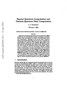
We briefly and informally revisit an extension to graphs, called pattern-graphs, which introduces a graphical notation for describing certain inductive families of graphs. A more detailed and formal account can be found in [6]. Pattern-graphs introduce a new notation, called !-box notation, which draws boxes around subsets of the vertices. These vertices are said to be in a !-box. Pattern graphs come with the following operations on !-boxes: Copy: !-boxes and the subgraph they contain may be copied arbitrarily many times. Any incident edges also get copied. Copying zero times removes their content and all incident edges. Drop: !-boxes may be thrown away, keeping their content. Merge: !-boxes may be merged to form larger bang boxes. The semantics of pattern-graphs is that they represent the inductive family of graphs without !-boxes that can be constructed by the transitive closure of the !-box operations. An illustration of these !-box operations is shown in Figure 1. The !-box notation lets pattern graphs express a limited form of inductive structure. In particular, it allows important equations from quantum computation to be expressed, such as the spider theorem described in section 2.2, which can be formally captured by the rules described in section 5.1. Like the underlying graphs of symmetric monoidal categories, pattern graphs let us express rewrite rules to form an algebraic structure over pattern graphs. These capture an infinite family of rewrites between graphs of the symmetric monoidal categories. For a pair of pattern graphs to form a meaningful rewrite, the following conditions are needed: 5

i1

i2

i3

≤ G

i4

≤ copy({i1 7→ 2}, G)

≤ merge({{i2 , i3 }}, G)

drop({i4 }, G)

Figure 1: An illustration of !-box graph matching using the !-box operations. This involves first copying !-box i0 twice, merging these two !-boxes and finally dropping the merged !-box. • Like the underlying graph formalism, there must be an isomorphism between exterior nodes in the left and right hand sides. • There must be a partial mapping between !-boxes on the left and right hand sides so that the unfolding used when matching a !-box on the left is applied to the mapped !-box on the right before replacement. This ensures that the replacement has the same interface as the original graph. • There must be a bijection between the exterior nodes in each !-box on the left hand side, with each vertices in the mapped !-box on right hand side. The fundamental property that rewriting must preserve, for equations over symmetric monoidal categories to be well formed, is that the interface, must remain unchanged. If an equation is used, then it cannot change the objects in the category. This ensures that composition commutes with rewriting, giving graph patterns the rich compositional structure of 2-categories.

4.1

Matching by Cutting

A useful intuition for matching is that a source graph matches a target graph when a part of the target graph can be cut-out such that it looks identical to the source graph. The crucial technical issue is that we may cut through both edges and vertices. When we cut through a vertex, we may throw away part of the graph which was connected by the incident edges. We also lose any content that was in the vertex. If it was an internal vertex, then it becomes and exterior vertex. Returning to the matching example considered in the previous section, the following cuts can be made:

⇒

6

The idea of matching is extended to !-box’s by allowing the source graph’s !-boxes to be expanded by the !-box rules before the target graph is cut up. Although, the !-boxes in the target may not be cut, their content may. However, the !-boxes in the expanded source must be in isomorphism with those in the cut-out subgraph of the target. Again, further details are in [6]

4.2

The Pattern Graph Matching Algorithm

While matching was proved to be decidable in [6], this proof results in an inefficient generate and test algorithm. Here, we present a more efficient algorithm based on a simultaneous traversal of the two graphs being matched and an incremental expansion of the !-boxes ‘on demand’. We call the graph that corresponds to the left hand side of a rewrite the source, and the graph it is matched against the target. Our algorithm breaks the matching process into a series of steps. Each step takes a matchstate and results in a list of alternative next matchstates. In each successive matchstate, another vertex of the source graph has been matched. There is choice in the matching process which is why the result is a list of possible partial matches. Exterior-vertices with exactly one incident edge, called leaf-vertices, are treated specially for pragmatic reasons: they can match any half-edge. This makes them the most flexible resource in matching. With this in mind, the matchstate is a datatype consisting of: agenda: a mapping from source to target vertices which is used as an agenda of nodes that still need to matched, initially empty. unm src: the source graph with vertices removed as they are matched, initially just the source graph. src lfs: unmatched leaf vertices from the initial source graph that have not yet been matched, initially all leaf vertices. unm tgt: the target graph with edges removed as they are matched, initially the full target graph. bboxmatch: a mapping from !-boxes in the source to !-boxes in the target, initially empty. match: a (partial) match of the underlying graph without !-boxes, initially empty. The invariants these elements are: • The agenda is a partial function V (unm src) 7→ V (unm tgt) (it maps a subset of the vertices in unm src to vertices unm tgt).

7

• src lfs is a subset of the vertices in unm src which are leaf vertices in the source graph. Because the algorithm involves removal of vertices from unm src new leaf-vertices in unm src might be introduced. Hence a separate collection of the original leaf vertices needs to be maintained. • match is a valid matching between a strict subgraph of the source and target graphs. The details of what constitutes a match are presented in [6]. • bboxmatch is a valid !-box match with respect to match (only vertices in the source !-box are mapped to corresponding vertices in target !-box). In particular, this an isomorphism from the expanded source graph’s !-boxes to the targets !-boxes. The top-level of the matching algorithm performs incremental match steps where each step compares a previously unseen vertex from the source to a vertex in the target graph. At each step, the matched edges are removed from the unm tgt, the matched vertices are removed from unm src (as well as all their incident edges), and any matched leaf vertices are also are removed from src lfs. The unm src and unm tgt graphs are used to allow an incremental search over the initial source and target graphs without having to consider vertices or edges more than once. The unm src graph is also used as a secondary agenda for the disjoint parts of the source graph that still need to be matched. Match Steps The top-level of the matching algorithm simply repeats matching steps, producing a lazy list of match-states. The match-step function has one base case: • if there are no more vertices in unm src then matching is complete, and the match and bboxmatch are returned. Otherwise, there are two possible step cases: • If agenda is empty, then a either matching has just started or a disconnected component has finished being matched, and in either of these cases, a new vertex is chosen from the source graph and matched, using the function match2vertices which is described below, against every possible vertex in the target graph. Each matching vertex in the target graph can result in a list of possible new matchstates. The flattened list is the result of the match step. • If agenda is not empty, then it contains a mapping from a source vertex to a target vertex. Matching these vertices, also done by the function match2vertices, results in a list of updated matchstates which are then the result of this match step.

8

Match Two Vertices The crucial operation for matching is function match2vertices which results in a list of new matchstates by attempting match a single vertex in the source graph against a given one in the target graph. This involves expanding any adjacent !-boxes as necessary, matching any optional vertex data, and also constructing maps for all incident edges, and adding any adjacent vertices to the agenda. Only extensions to matching which are consistent with the existing matchstate are returned. If there are no consistent extensions to matching with the two given vertices, it is said to fail and the empty list is returned. The matched vertices and edges, from unm src and unm tgt respectively, are also removed. All the edges from unm src must be matched although some edges may remain in unm tgt - this is why vertices cannot be removed from unm tgt. Local !-box Expansion The first operation is to consider expanding any !-boxes which are adjacent to the source vertex being considered. When the source vertex is an exterior one, then extra edges in the target are allowed. All combinations of expansions of the adjacent !-boxes are considered as long as the resulting arity (number of incident edges) is less than the matched target vertex. If the source vertex internal, then the !-box expansion must result in the target vertex having exactly the same arity as the target vertex. Self-loops The second operation is to match all the self-loops of the source vertex. 1. If the target vertex has fewer self-loops, then matching fails. 2. If the target vertex has exactly the same number of self-loops, then the self-loops are removed from the target. 3. If the target vertex has more self-loops, and the source vertex is internal, then the only way to match the extra-self loops is with leaf vertices adjacent to the source vertex. 4. If the target vertex has more self-loops, and the source vertex is external, then any even number of the source’s leaf vertices can be used to match the self-loops (it requires two leaf vertices to match one self-loop). Any additional target vertices remain unmatched. All !-boxes around leaf vertices which are matched to self-loops get dropped. Once self-loops have been matched, all self-loops are to be removed from the unm src and unm tgt graphs.

9

Adjacent Vertices The third operation is to pair-up adjacent vertices in the source and target and add these to the agenda. Only pairings that respect the edges are allowed. This is done by considering the adjacent vertices in the target graph first. The reason is that when the source vertex is exterior, then target vertices can be ignored. Recursion on the adjacent source vertices cannot decide in advance which target vertices to ignore, and would thus result in repeated, but identical, matches. When the source vertex is exterior, target vertices can be ignored provided that all source vertices are still matched. Every permissible combination of target vertices is considered as an option to be ignored. For each adjacent target vertex that is not ignored, there is a choice of each adjacent pattern vertex to try to pair it up with. Furthermore, when there are multiple adjacent exterior source vertices, any combination of them can be paired against the adjacent target, provided that all edges are matched. All combinations must be consisted for matching to be complete. Any adjacent vertices that are in the same source !-box, must be paired and then matched to a vertex in the corresponding target !-box. The !-box mappings are stored as an injective map from source !-boxes to target !-boxes. This implicitly defines the merges by multiple source !-boxes matching the same target !-box.

4.3

Properties of Matching

There are a number of properties we would like to prove for pattern graph matching. Proving soundness would ensure that only valid matches are produced. This could be proved inductively for each part of the algorithm. In particular, that the matchstate always represents a valid match if the source graph’s vertices held in the agenda are assumed to consist only of exterior vertices, with no additional edges. The algorithm’s termination with an empty agenda then ensures that the final matchstate is a valid match for the whole of the source graph. Proving completeness would ensure that all matches are found. Again an inductive proof can be performed to show that every initial match is found and then every extension to the match is considered. Proving minimality would ensure that every match produced is different (with respect to the identity of the underlying vertices and edges). This can be proved by showing that each step has produced a unique extension to the matching. Because the algorithm is deterministic and only has branches when part of the match is extended uniquely, no two matches will be the same. Minimality with respect to edge-identity produces many additional symmetries when edges contain no data. For this reason it is interesting to consider the stronger minimality criteria of vertex-minimality: every match found is different with respect to the edge-matching. Our implementation is vertex-minimal by treating edges as a uniform resource, essentially as a number, which is decreased to zero when all edges are matched.

10

The development of full proofs of soundness, completeness, and minimality is still future work.

5

Quantum Computation

Quantum computation is the a field of study concerned with the use of data derived from quantum systems (e.g. particle measurement outcomes) to perform computations. This field operates largely (but not totally) in the context of Hilbert space quantum mechanics, where states are represented as vectors in a Hilbert space, state evolutions are represented as unitary linear maps, and measurements as sets of projections. Here, we shall focus on computations where the single-system state space is the two dimensional complex Hilbert space C2 . This is called the space of qubits, the quantum analogue of bits. We can form compound systems by taking tensor products. Furthermore, the category FdHilb of finite-dimensional Hilbert spaces is a monoidal category, taking the usual tensor product as ⊗ and C as the unit. For this reason, we regard C as the empty system. For Hilbert spaces H1 , H2 , let Ψ ∈ H1 ⊗ H2 . If there exists ψ ∈ H1 , ϕ ∈ H2 such that Ψ = ψ ⊗ ϕ, then we say Ψ is separable. If there exist no such ψ, ϕ, we say Ψ is entangled. In the space C2 ⊗ C2 , an example of an entangled state is the Bell state Ψ0 := e1 ⊗ e1 + e2 ⊗ e2 , for {e1 , e2 } an orthonormal basis. Entanglement is essential to quantum computation, as it provides a mechanism for information to flow from one system to another. Notice how the map F : C2 → C2 seems to “flow” across the Bell state:2 (F ⊗ 1C2 )(e1 ⊗ e1 + e2 ⊗ e2 ) = (1C2 ⊗ F T )(e1 ⊗ e1 + e2 ⊗ e2 ) This effect is exploited in protocols such as quantum teleportation, justifying the point of view that bipartite entangled states are like wires. Tripartite states are then like junctions. One state that is particularly useful in the capacity is the Greenberger–Horne–Zeilinger (GHZ) state: e1 ⊗ e1 ⊗ e1 + e2 ⊗ e2 ⊗ e2 Where {e1 , e2 } is an orthonormal basis. We say a state is symmetric when it is invariant under permutation of qubits. We now have the following result. Theorem 2. Symmetric GHZ states are in 1-to-1 correspondence with the special commutative frobenius algebras on C2 . By the usual category theory trick, we shall regard vectors in a Hilbert space H as arrows from the tensor unit C into H. Then, for any symmetric GHZ state Ψ, there exists a unique special commutative frobenius algebra on C2 , such that: 2 Here,

we take (−)T to be transposition in the ei basis.

11

=Ψ

Conversely, any SCFA generates a GHZ state as above.

5.1

A Rewrite Theory

We are now equipped to express a rewrite theory for GHZ dots. Let green dots represent the SCFA generated by the GHZ state from the previous section. These first two rewrites follow from the properties of a CFA. The third rewrite follows from specialness, and gives the full spider theorem.

→

→

→

However, this rewrite system on its own isn’t particularly enlightening. The spider theorem already tells us what it will do, i.e. collapse connected graphs to a single dot. The story becomes more interesting when we introduce a second GHZ state. Define a new orthonormal basis √ √ d1 := 1/ 2 (e1 + e2 ) d2 := 1/ 2 (e1 − e2 ) Let the GHZ state defined on this basis (and the induced SCFA) be represented by red dots. Now, in addition to the three rules above, we have the following identities.

→

→

These and several other rules follow from the fact that the red dots and the green dots correspond to complementary observables. These have a rich (mostly) abstract theory, and can be used to reason about how classical data interacts with quantum systems. For details, see [3, 5].

12

Figure 2: A screenshot of Quantomatic performing a rewrite.

6

Quantomatic

Quantomatic is a tool for automatically performing rewrites on graphical expressions in a monoidal category. After a ruleset, such as the one in this paper, has been imported, the user can manually do rewriting on a graph or a portion of a graph, or he can ask Quantomatic to normalised with respect to all of the activated rules. It also supports attaching expression data, such as phase angles (see [3]) to vertices. To aid in the expansion of a rewrite theory, Quantomatic also interfaces with a Mathematica library to evaluate graphs in the matrix semantics, evaluate entanglement metrics, perform partial traces, solve for free phases, and do many other quantum-information-related tasks. Development is ongoing to implement a full-featured theory editor and a richer matching engine that supports a broader range of pattern-graph-based rulesets.

7

Conclusions and Further Work

We have sketched the relationship between graphs and monoidal categories and highlighted how inductive structure can be formalised to provide a formal theory for rewriting families of graphs. We outlined an algorithm for matching based on

13

graph traversal. This expands !-boxes on demand. Important properties of this algorithm are suggested and proof sketches provided. The utility of using this rewriting mechanism for reasoning about quantum information was presented and the Quantomatic tool was introduced which implements these ideas. Further work includes filling out the sketched proofs for the properties of matching as well as improving the efficiency of matching by observing symmetries in rewrite rules. Developing graph-indexing techniques for the monoidal setting is another important algorithmic challenge.

References [1] Samson Abramsky and Bob Coecke. A categorical semantics of quantum protocols. In Proceedings from LiCS, arXiv:quant-ph/0402130v5, Feb 2004. [2] Bob Coecke. Kindergarten quantum mechanics. arXiv:quant-ph/0510032v1, 2005. [3] Bob Coecke and Ross Duncan. Interacting quantum observables: Categorical algebra and diagrammatics. arXiv:0906.4725v1 [quant-ph], 2009. [4] Bob Coecke, Eric Oliver Paquette, and Dusko Pavlovic. Classical and quantum structuralism. Semantic Techniques for Quantum Computation, page 43, Oct 2008. [5] Bob Coecke, Eric Oliver Paquette, and Simon Perdrix. Bases in diagrammatic quantum protocols. arXiv:0808.1029v1 [quant-ph], Aug 2008. [6] Lucas Dixon and Ross Duncan. Extending graphical representations for compact closed categories with applications to symbolic quantum computation. AISC/MKM/Calculemus, pages 77–92, Jun 2008. [7] Peter Selinger. Dagger compact closed categories and completely positive maps (extended abstract). Electronic Notes in Theoretical Computer Science, 170:139–163, 2007. [8] Peter Selinger. A survey of graphical languages for monoidal categories. http://www.mscs.dal.ca/∼selinger/papers.html, 2009.

14