MONTE CARLO BAYESIAN FILTERING AND SMOOTHING FOR TVAR SIGNALS IN SYMMETRIC α-STABLE NOISE Marco J. Lombardi∗ and Simon J. Godsill Signal Processing Laboratory Department of Engineering University of Cambridge Trumpington Street CB2 1PZ Cambridge, U.K. (Europe) phone: +44 1223 332604, fax: +44 1223 332662, email:
[email protected] web: www-sigproc.eng.cam.ac.uk/˜sjg/
Dipartimento di Statistica “G. Parenti” Universit`a degli studi di Firenze Viale G.B. Morgagni 59 I-50134 Firenze, Italy (Europe) phone: +39 055 4237256, fax: +39 055 4223560, email:
[email protected] web: www.ds.unifi.it/˜mjl/
ABSTRACT In this paper we propose an on-line Bayesian filtering and smoothing method for time series models with heavy-tailed alpha-stable noise, with a particular focus on TVAR models. We first point out how a filter that fails to take into account the heavy-tailed character of the noise performs poorly and then examine how an α-stable based particle filter can be devised to overcome this problem. The filtering methodology is based on a scale mixtures of normals (SMiN) representation of the α-stable distribution, which allows efficient RaoBlackwellised implementation within a conditionally Gaussian framework, and requires no direct evaluation of the αstable density, which is in general unavailable in closed form. The methodology is shown to work well, outperforming the traditional Gaussian methods both on simulated and real audio data. The analysis of real degraded audio samples highlights the fact that α-stable distributions are particularly well suited for noise modelling in a realistic scenario. 1. INTRODUCTION In many real signal processing environments, sources of noise cannot be considered as Gaussian. Here we consider in particular the estimation of processes observed in heavy-tailed noise, i.e. noise having occasional very large values that could strongly affect any inference procedure for the underlying process. We focus on one particular class of heavy-tailed distribution, the symmetric α-stable class, that can be obtained through a generalisation of the central limit theorem when the random variables need not have finite variance, see [7, 22]. Such noise processes have been found appropriate in a number of areas, including signal processing [20] and econometrics [23]. We propose methodology for optimal on-line estimation of stochastic processes observed in α-stable noise. The models chosen are time varying autoregressions (TVAR), which are appropriate for a wide range of signals, including speech, audio, eeg and seismic data. On-line estimation and signal extraction is performed by means of sequential Monte Carlo methods [11, 13, 4]. These methods have been applied to the TVAR model with Gaussian noise in [6, 24, 10]. This paper constitutes an extension to these approaches (and especially that of [24]) to the symmetric α-stable case and, more generally, to any case where the noise distribution ∗ This paper was completed when the first author was visitng the Signal Processing lab at the University of Cambridge. We are indebted to Jaco Vermaak for allowing us to exploit and modify his Matlab source code.
can be represented as a scale mixture of normals (SMiN). The SMiN representation of the α-stable class allows us importantly to employ conditionally linear and Gaussian computational methods within the Monte Carlo filter (via the Kalman filter), hence avoiding any direct evaluations of the noise density function (which is unavailable in most cases for the α-stable model). In [9](see also further references on www-sigproc.eng.cam.ac.uk/sjg) methodology was presented for inference about static AR models in stable law noise. Here this methodology is extended to the sequential Monte Carlo setting for TVAR models in α-stable noise. The methods are able accurately to reconstruct the signal process, the TVAR parameters, and also the stable law parameter α, which is static and thus not easily amenable to particle filter analysis. A real application of the methods is presented for audio signal enhancement. We present compelling experimental evidence that the α-stable distribution is appropriate for certain noise sources in 78rpm gramophone disk recordings which are typically degraded by non-Gaussian clicks. Results are found to be very effective. The structure of the paper is as follows: we begin describing the properties of α-stable distributions and proposing that they are more appropriate than other parametric families in modelling noise in certain audio sources. We then introduce the statistical model and its state-space representation. Bayesian methods are presented for sequential estimation and filtering and we discuss how symmetric αstable distributions can be embedded into this framework. The approach is then compared to the traditional Gaussian framework on both simulated data and artificially corrupted audio samples. An application to real audio data concludes the paper.
2. α-STABLE DISTRIBUTIONS The α-stable family of distributions stems from a more general version of the “traditional” central limit theorem in which the assumption of finite variance is replaced by a much less restrictive one concerning the regular behavior of the tails [7]; the Gaussian distribution then becomes a particular case of α-stable distribution. This family of distributions has a very interesting pattern of shapes, allowing for asymmetry and thick tails, that makes them suitable for the modelling of several phenomena; moreover, it is closed under linear combinations. The family is identified by means of the characteristic
865
function ½ © ¤ª £ πα exp ©iδt − γ α |t|£α 1 − iβsgn(t) tan ¤ª 2 ϕ(t) = 2 exp iδt − γ|t| 1 + iβ π sgn(t) ln |t|
α 6= 1 α=1 (1) which depends on four parameters: α ∈ (0, 2], measuring the tail thickness (thicker tails for smaller values of the parameter), β ∈ [−1, 1] determining the degree and sign of asymmetry, γ > 0 (scale) and δ ∈ IR (location). To denote a stable distribution with parameters α, β, γ and δ we will use the shorthand notation S(α, β, γ, δ). As in the Gaussian case, a random variable X with S(α, β, γ, δ) distribution can be standardized to produce X −δ ∼ S(α, β, 1, 0). Z= γ For the standardized stable distribution, we will henceforth use the shorthand notation S(α, β). Unfortunately, (1) can be inverted to yield a closed-form density function only for a very few cases: α = 2, corresponding to the normal distribution, α = 1 and β = 0, yielding the Cauchy distribution, and α = 12 , β = 1 for the L´evy distribution. This difficulty, coupled with the fact that moments of order greater than α do not exist whenever α 6= 2, has made impossible the use of “traditional” estimation methods such as maximum likelihood and the method of moments. Researchers have thus devised alternative estimation methods, mainly based on quantiles [17], the performance of which is judged unsatisfactory in a number of respects, especially because they are not liable to be incorporated in complex models and thus require a two-step estimation approach. With the availability of powerful computing machines, it has become possible to devise computationally-intensive estimation methods for the estimation of α-stable distributions, such as maximum likelihood based on the FFT of the characteristic function, as in [18], or direct numerical integration as in [21]. These methods, however, present some inconvenience: the accuracy of both the FFT and the numerical integration of the characteristic function is quite poor for small values of α because of the spikiness of the density function; furthermore, when the parameters are near their boundary, their distributions assume non-standard form, making traditional confidence intervals unreliable. Given these computational difficulties, it is perhaps surprising that simulated values from α-stable distributions can be straightforwardly produced with a simple analytic transformation of two uniformly distributed random numbers [3]. The possibility of a simulation based Bayesian approach was first put forth in [2], who shows how to devise an auxiliary variable conditional on which the likelihood can be expressed in closed form. Unfortunately, simulated values from this auxiliary variable cannot readily be generated and one must resort to more elaborate sampling methods. Furthermore, several reparameterizations are needed in order to obtain posterior distributions that can be easily simulated from. This makes the whole procedure quite slow, especially when large sample sizes are involved. In the case of symmetric stable distributions, the situation is much less cumbersome: we can exploit the fact that a symmetric α-stable distribution can be represented as a scale mixture of normals (SMiN) [1]; this observation will enable the efficient conditionally Gaussian simulation techniques proposed later. To put it in a more formal way, let us consider a generic model with symmetric α-stable noise
SMiN property allows us to express the α-stable noise equivalently as √ ² i = δ + γ λ i ui ,
λi ∼ S
¡α 2
¢ , 1 , ui ∼ N (0, 1).
¡ ¢ where λi and its positive stable distribution S α2 , 1 are known as the mixing parameter and the mixing distribution, respectively. Conditionally on λi , we have thus ²i |λi ∼ N (δ, γ 2 λi ).
(2)
and hence in a Monte Carlo environment we will be able to utilise efficient normal/linear computations while avoiding entirely the need to evaluate S(α, 0, γ, δ). It is worth noting that this SMiN representation is exact, and does not involve any approximations such as would be induced through the use of the better known finite mixture of normals approach to heavy-tailed noise modelling. 2.1 Justification for use of α-stable distributions in audio applications The above theoretical arguments in favor of α-stable distributions are supported in our application by a very good fit to real noise data. The noisy data is taken from 78rpm recordings of ethnomusicological sources carried out by Lachmann in the early 20th century. An excerpt of just over one second (44487 observations) of the recording, in which there was no musical signal present, was extracted and fitted to a stable distribution, using an approximate maximum likelihood method based on the FFT of the characteristic function1 . Results are reported in table 1, along with the estimated parameters for a simple Gaussian and a more standard heavytailed Student’s t model. In figure 1 we report the kernel density estimate of the dataset and the normal, the Student’s t and the stable fitted densities. Although not very far from normality, the stable distribution provides a much better fit both in the central part and in the tails of the distribution with respect to both the Gaussian and the Student’s t model. The estimation output of the α-stable model also highlighted a mild degree of negative asymmetry, but in order to be able to exploit the mixture of normals representation we will restrict our attention, in what follows, to the symmetric case. Table 1: Maximum likelihood estimates of an α-stable distribution and test statistics for different null hypotheses. α-Stable Student’s t Gaussian Est. Std. err. Est. Est. α 1.8352 0.0062 ν 5.5145 β -0.2226 0.0282 µ 0.1006 µ 0.0166 γ 3.6343 0.0108 σ 4.6706 σ 5.9642 δ -0.0181 0.0173 -1.0457
3. STATISTICAL MODELS
²i ∼ S(α, 0, γ, δ).
AR processes have been widely and successfully used in the setting of audio enhancememt [8] (and in many other areas of signal processing). Here we adopt the time-varying autoregressive (TVAR) process, in which the AR coefficients evolve over time according to certain specified dynamics. Models of this type have been employed in signal processing by, amongst others, [6], [12] and [19]. The audio signal
If we introduce an auxiliary white noise ui ∼ N (0, 1), where N (0, 1) denotes a standard normal distribution, the above
1 For a more detailed description on how the maximum likelihood procedure is implemented, we refer to [16].
866
−4
0.05
0.08
8
f(x)
f(x) 0.07
so that the model is expressed in conditionally Gaussian state space form. According to this approach, λt would be treated as a unknown parameter and incorporated into θt . The evolution of θt over time (excluding λt ) obeys a first order Markov process, whose parameters are assumed to be fixed and known:
x 10
f(x)
0.04 6
0.06 0.03
0.05
4
0.04
p(θ0 ) p(θt |θt−1 )
0.02
0.03
2
0.02
p(a0 )p(φ²0 )p(φη0 )p(λ0 ) p(at |at−1 )p(φ²t |φ²t−1 )p(φηt |φηt−1 )p(λt )
0.01
with
0.01 0 −20
= =
x
0
20
0
5
15
10
x 20
0 20
25
x 30
Figure 1: Kernel density (solid line), Gaussian fit (grey line), Student’s t fit (dashed line) and α-stable fit (dotted line).
p(φ²0 ) = N (0, δ²20 )
p(φ²t |φ²t−1 ) = N (φ²t−1 , δ²2 ) (8)
p(φη0 ) = N (0, δη20 )
p(φηt |φηt−1 ) = N (φηt−1 , δη2 )
p(λt ) = S( α2 , 1)
p(a0 ) ∝ N (0, ∆a0 )1Ia0 ∈Ap
p(at |at−1 ) ∝ N (at−1 , ∆a )1Iat ∈Ap . at time t is thus modelled as a TVAR (p) process xt =
p X
ak,t xt−k + σ²t ²t ,
²t ∼ N (0, 1),
4. SEQUENTIAL MONTE CARLO METHODS (3)
k=1
and is burued in symmetric α-stable noise such that the observations are yt = xt + γηt ηt ,
ηt ∼ S(α, 0),
(4)
where σ²t and γηt represent, respectively, the standard deviation of the innovations in the true signal process and the scale of the stable noise; both are allowed to be time-varying. We furthermore assume that ²t and ηt are independent. The time-varying parameter vector of the model thus has dimension p + 2 and is given by θ t = (at , φ²t , φηt ) ,
θt ∈ {Ap × IR × IR}
We have already stated that our main goal is to reconstruct, on the basis of the observable noisy signal, the unobservable clean signal. One could be interested in simply obtaining a point estimate x ˆt for every time interval, but in Bayesian terms it is much more interesting to focus our analysis on the filtering distribution p(ˇ xt , θt |y1:t ) or on the fixed-lag smoothing distribution p(ˇ xt , θt |y1:t+L ), on the basis of which we can construct both point estimates and HPD intervals for xt , for example. Expressed in the above formulation, the model is not linear and closed-form algorithms such as the Kalman filter cannot be employed. However, it is immediately observed that, conditionally on θ0:t , the model is linear and Gaussian; p(ˇ xt |θ0:t , y1:t ) can thus be obtained analytically using the Kalman filter. The Kalman filter runs as follows: for k = 1, . . . , t we first set the sufficient statistics for the predictive distributions
with at = (a1,t , a2,t , . . . , ap,t )
φ²t = ln σ²2t ,
φηt = ln γη2t ;
where Ap is the region of stability of a stationary AR(p) process2 . The above model can be readily expressed in state-space form. The system matrices are · ¸ · ¸ σ²t a0t At = Bt = 0k−1×1 Ip−1 0k−1×1 C = [1 0k−1×1 ]
Dt = [γηt ]
vt ∼ N (0, I) ut ∼ S(α, 0).
(5) (6)
Now, exploiting the mixture of normal representation of a stable distribution (2), we can redefine h √ i ¡ ¢ D?t = γηt λt λt ∼ S α2 , 1 and express (6) exactly equivalently as yt = Cˇ xt + D?t wt
wt ∼ N (0, I),
Ak mk−1|k−1
Pk|k−1 (θ0:k ) yk|k−1 (θ0:k )
= =
Ak Pk−1|k−1 A0k + Bk B0k Cmk|k−1 ;
Sk (θ0:k ) = CPk|k−1 C0 + D?k D?0 k , and we finally obtain the parameters of the filtering distribution according to mk|k (θ0:k )
=
¡ ¢ mk|k−1 + Pk|k−1 C0 S−1 yk − yk|k−1 k
Pk|k (θ0:k )
=
Pk|k−1 − Pk−1|k−1 C0 S−1 k CPk|k−1 .
The filtering distribution of the state vector is thus ¡ ¢ p(ˇ xk |θ0:k , y1:k ) = N mk|k , Pk|k ,
(9)
and the likelihood of the last observation is ¡ ¢ p(yk |θ0:k , y1:k−1 ) = N Ak mk|k , D?k + Ak Pk|k A0k . (10) Now, since
(7)
2 This condition is only sufficient and not necessary when dealing with TVAR processes. However, regions of stability for TVAR processes are much more complex to deal with, so we have decided to enforce this simpler condition.
=
we compute
and, defining x ˇt = (xt , xt−1 , . . . , xt−p+1 ), x ˇt = At x ˇt−1 + Bt vt yt = Cˇ xt + Dt ut
mk|k−1 (θ0:k )
p(ˇ xt , θ0:t |y1:t ) = p(ˇ xt |θ0:t , y1:t )p(θ0:t |y1:t ), the problem reduces to one of obtaining simulated values from p(θ0:t |y1:t ) in order to produce a random sample to
867
be used for Monte Carlo inference3 . This is in general difficult, and an importance sampling technique can be employed. Given a probability distribution π(θ0:t |y1:t ) which is easy to simulate from, we produce a set of M random vectors θ0:t from it and assign to each one a weight w0:t (θ0:t ) ∝
p(θ0:t |y1:t ) π(θ0:t |y1:t )
to be used in Monte Carlo inference. 4.1 Particle Filters In the above framework the data are processed in batches and, as new observations arrive, it is necessary to produce a new sample from the importance distribution (with increasingly large sample size) and reassign the importance weights. In many practical situations, however, ranging from the signal processing to the financial field, data are available on a sequential basis, and having to re-run the whole estimation as new data arrives is often not feasible when new observations arrive at a high rate. Particle filtering methods have been recently rediscovered in independent work by [11] and [13]. The idea underlying this approach is to represent the distribution of interest by a large number of particles evolving over time on the basis of a simulation-based updating scheme, so that new observations are incorporated in the filter as they become available. More formally, the objective is to update, at each time interval, p(θ0:t |y1:t ) without modifying the past values of θ. The importance distribution should thus be such that π(θ0:t |y1:t ) = π(θ0:t−1 |y1:t−1 )π(θt |θ0:t−1 , y1:t ), and the weights factorise as w(θ0:t ) = w(θ0:t−1 )wt where wt ∝
p(yt |θ0:t , y1:t−1 )p(θt |θt−1 ) . π(θt |θ0:t−1 , y1:t )
The weights can then be updated recursively, since w(θ0:t ) = w(θ0:t−1 )wt . It was shown in [4] that the optimal importance distribution, that is the one that minimizes the variance of the importance weights, is p(θt |θ0:t−1 , yt ). Unfortunately, this is not easy to simulate from. A simple alternative, as employed in [11, 13], is to use π(θt |θ0:t−1 , y1:t ) = p(θt |θt−1 ), wt ∝ p(yt |θ0:t , y1:t−1 ) i.e. the importance weights are then simply proportional to the marginal likelihood. The weights are then normalized according to ³ w ˜
(i) θ0:t
´
³
(i)
w θ0:t ´, ³ = P (j) M j=1 w θ0:t
(i)
3 This
It turns out that an algorithm of this kind will eventually degenerate, i.e. assign almost all the weight to a single particle. In order to overcome this problem, a resampling step is necessary. In the resampling step, particles with low importance weights are discarded and those with high importance are multiplied. More formally, after producing a set of particles from the importance distribution and having assigned to each one an appropriate weight, we associate P to each particle i a number of offsprings Mi such that M i=1 Mi = M . After this selection step, offspring particles replace the original particles and the importance weights are reset to 1/M , so that the set of particles can be thought of as a random sample. The resampling step can be implemented at every time interval [11], or it can be employed whenever the set of particles crosses a certain degeneracy threshold. A measure of degeneracy of the algorithm is the effective sample size [15], defined as M Me = . 1 + Var(wt ) This quantity can be estimated by ˆe = P 1 M ; 2(i) M ˜t i=1 w ˆ e drops below a certain threshold, the resampling when M takes place. Several different sampling schemes have been proposed in (i) the literature. In the following, we will denote with θ˜t the i-th particle, as sampled from the importance distribution, (i) at time t, and with w ˜t its associated normalized importance weight. In our work, we have employed Systematic sampling, which has smaller variance with respect to other schemes [24]. The number of offsprings is taken to be proportional to the importance weight and is generated by simulating a set U of M uniformly distributed random variables on [0, 1], taking the cumulated sum of the normalized weights qi =
is an example of the Rao – Blackwellized procedure, see
i X
(j)
w ˜t ,
j=1
and then setting Mi equal to the number of points in U that fall between qi−1 and qi . In this case the variance is ´ ³ 0(i) ¯ wt0(i) . ¯w 1−M Var(Mi ) = M ˜t To wrap up, what the algorithm practically implements at each time interval is the following: 1. Sample M particles θt† from the importance distribution † π(θt |θ0:t−1 , y1:t ) and set θ0:t = (θt† , θ0:t−1 ). 2. Evaluate the importance weights according to wt ∝
´
where θ0:t denotes the i-th particle. This is basically the approach employed in the seminal paper by [11], plus the resampling step which we will discuss in the following paragraph.
[4].
4.2 Resampling
† p(yt |θ0:t , y1:t−1 )p(θt† |θt−1 ) . π(θt† |θ0:t−1 , y1:t )
3. Normalize the importance weights: ´ ³ (i) w θ0:t (i) ´. ³ w(θ ˜ 0:t ) = P (j) M j=1 w θ0:t ˆ e below threshold by multiplying or dis4. Resample if M carding particles according to their weight to produce a new set of M particles θ0:t , each with weight w(θ ˜ 0:t ) = 1/M .
868
An issue which is closely related to degeneracy is that of the depletion of samples. When performing the resampling step, particles with high importance weight tend to be sampled a large number of times and it could happen that the initial set of particles ends up in collapsing into a single particle. A method to overcome this problem [14] is to sample from a kernel smoothed estimate of the target density, computed on the basis of the current set of particles. However, the drawback of this approach is that, besides raising problems concerning the choice of a specific kernel and bandwidth, it increases the Monte Carlo variance. We will examine in what follows two situations in which the depletion of samples should be seriously taken into account. 4.3 Fixed-lag smoothing In some cases, in order to obtain a smoother estimate of the state, it is useful to consider the distribution at time t after a certain number of time intervals L. In more formal terms, instead of considering p(ˇ xt |y1:t ), we focus on p(ˇ xt |y1:t+L ). It is hoped that expanding the information set by the use of an appropriately chosen lag window L improves the estimates of the states. In principle, fixed-lag smoothed densities can be straightforwardly obtained by the general algorithm proposed above, by simply extracting signal estimates at time t − L + 1 from the particles. However, it turns out that such a scheme, where states at time t − L + 1 could have been resampled up to L times, leads to serious degeneracy as L grows larger. In order to overcome this degeneracy problem, an MCMC approach similar to [24] can be adopted. Let us consider that, at time t + L, the particles are distributed according to p(θ0:t+L |y1:t+L ); the idea is to apply to each particle a Markov transition kernel K ∗ with invariance distribution p(θ0:t+L , y1:t+L ) in order to introduce diversity among the particles. 0(i) If we denote with θ0:t+L the i-th particle after the resampling stage, the MCMC proceeds by sampling each particle (i) (i) and state θk according to target density p(θk |θ−k , y1:t+L ), where ´ ³ (i) 0(i) 0(i) (i) 0(i) (i) θ−k = θ0:t−1 , θt , . . . , θk−1 , θk+1 , . . . , θt+L , and k = t, t + 1, . . . , t + L. A Metropolis-within Gibbs sampling MCMC scheme is used to achieve this and full details, including the forward-backward Kalman filter for efficient implementation, may be found in[24]. 4.4 Static parameters The degeneracy problem is however much more severe whenever the particle filter has to deal with the estimation of static parameters. The prior p(θt+1 |θt ) would have probability mass 1 at θt , so the particles are never updated and rejuvenated and they eventually collapse on a few – and sometimes even one – single value. In our specific case, we have up to now assumed the stable law tail parameter α to be known. This is rarely the case in practical applications. Furthermore, whereas in static estimation problems one could somehow pre-estimate static parameters, in our sequential estimation case this is obviously impossible. Fixing the static parameters to arbitrarily chosen guesses is in general very bad practice. In our specific case, however, a few experiments, not reported here for sake of brevity, have reported that, even if the guessed α is not very close to the actual one, the results are still satisfactory and the improvement in the SNR remains at the same order of magnitude. However, it would surely be preferable to estimate α together with the other parameters as the data are processed. Several approaches to this problem are available. The MCMC schemes above for fixed lag smoothing can be
adapted to the static parameter case, for example, although in our case this led to a filter of ever growing computational complexity and so was not adopted. Another approach to overcome the degeneracy problem is to introduce artificial parameter evolution, that is, simply pretending that static parameters are indeed time-varying by adding a noise term at each time interval. The problem is that in doing so we introduce additional variability by “throwing away” information. [14] propose a method for quantifying this loss of information and devise an artificial parameter evolution scheme immune to this problem. To focus the attention on our specific case, we note that the static parameter is the stability index α. Introducing artificial parameter evolution is equivalent to consider a model in which α is replaced by its time-varying analog αt which evolves according to αt = αt−1 + ζt ,
ζt ∼ N (0, ωt ).
In a situation in which α is fixed, the posterior distribution p(α|y1:t ) could be characterized by its Monte Carlo mean and variance α ¯ t and s2t . It is immediate to observe that, in the case of artificial parameter evolution, the Monte Carlo variance increases to s2t + ωt . The Monte Carlo approximation can be expressed as kernel smoothed density of the particles as p(α|y1:t ) ≈
M X
´ ³ (j) (j) κt N αt+1 |αt , ωt .
j=1
Now the target variance s2t can be expressed as s2t = s2t−1 + ωt + 2Cov(αt−1 , ζt ), so if we choose
ωt 2 we have managed to avoid the loss of information. A simple particular case in which this can be achieved is to consider µ ¶ 1 ωt = s2t −1 , δ Cov(αt−1 , ζt ) = −
where δ is a discount factor in (0, 1]; the authors suggest its value to be chosen around 0.95-0.99. If we define d = 3δ−1 , 2δ the conditional density evolution becomes ¢ ¡ p(αt+1 |αt ) ∼ N αt+1 |dαt + (1 − d)α ¯ t , h2 s2t , (11) where
µ h2 = 1 − d2 = 1 −
3δ − 1 2δ
¶2 ,
so that sampling from (11) is equivalent to sampling from a kernel smoothed density in which the smoothing parameter h is controlled via the discount factor δ. 5. EXPERIMENTS AND RESULTS In this section we will show how the sequential Monte Carlo method outlined above performs on both simulated and real audio data. As a benchmark of model performance, we will use the signal to noise ratio, defined as PT x2t SNR = 10 log10 PT t=1 , 2 t=1 (xt − zt ) where xt is the clean signal and zt represents, in turn, the observed noisy signal and the filtered state. We will start by considering the simplest case, that is the one in which α is
869
Signal sequence
x
6
x
6 4
4
2
2
0
0
−2
−2
−4
−4
−6
−6 0
20
40
60
80
100
120
140
160
180
t
200
Observed sequence
10
0
20
40
60
80
100
120
140
160
180
t
200
Figure 3: Filtered signal (solid line) with 95% quantile bands (dotted lines), stable noise, α = 1.4.
y 5 0 −5
2
−10
α 1.5
−15 −20
0
20
40
60
80
100
120
140
160
180
1
200
t
0
20
40
60
80
100
120
140
160
180
0.5 a
t
0
3
−0.5
Figure 2: Clean and noisy signal, synthetic data.
−1 −1.5
ε
4 Values of α smaller than 0.2 were ruled out in order to avoid overflows.
0
20
40
60
80
100
120
140
160
t180
3
σ
known a priori and we do not perform fixed-lag smoothing, so that there is no need for the MCMC step outlined in the above subsection. The importance function was taken to be the prior p(θt |θt−1 ); as a resampling scheme, we will use systematic sampling, applied at each time step. We have generated a synthetic signal of 200 observations with parameters ∆a0 = 2I, ∆a = 0.0005I, δ²20 = 0.2, δ²2 = 0.005, δη20 = 0.5, δη2 = 0.00005; the signal was then corrupted with symmetric α-stable noise with α = 1.4. The SNR of the noisy observations was 0.83dB. The synthetic data are depicted in figure 2. Using a simple Gaussian model, as the one proposed by [24], obviously leads to poor results. Especially when the signal is highly corrupted by the noise peaks, the filtered states are very near to the observations, according to the low likelihood of such extreme values under the Gaussian noise assumption. Furthermore the extreme observations are somehow “absorbed” by jumps in the variance of the signal. The overall improvement in SNR was of 0.86dB, with RMSE 1.6947. On the other hand, the use of the stable model greatly reduces the influence of the extreme noise observations, achieving a SNR improvement of 5.12dB with RMSE 1.0382; in particular, we note that the filter is not misled by extreme observations as it happened in the Gaussian case. Similar results hold when α is estimated along with the other parameters. The prior we used for α was a simple uniform distribution on [0.2, 2]4 , and we fixed the discount factor δ in (11) to 0.95. The evolution of the stability index is depicted in the top graph of figure 4 along with the 95% quantile bands. The SNR improvement is 5.13dB with RMSE 1.0372, nearly identical to the case analyzed earlier in which we fixed α to its true value. The evolution of the kernel smoothed posterior distribution of α in for the last intervals is presented in figure 5. In order to get insights about the appropriate number of particles to be used, we have performed a Monte Carlo experiment consisting of 50 independent replications. All experiments were performed on a laptop computer with a r r IV processor with 512Mb RAM. Pentium° 2.66GHz Intel° The results, reported in Table 2 seem to indicate that using more than 300 particles does not lead to a significantly
200 a 1 a 2 a
200
2 1 0
0
20
40
60
80
100
120
140
160
180
t
0.5
200
γ
η
0.4 0.3 20
40
60
80
100
120
140
160
180
t
200
Figure 4: Estimated parameters of the model, stable noise.
improved performance despite the increase in computational effort. A number of particles between 100 and 300 seems to be a good compromise between speed and accuracy. Table 2: RMSE and mean and standard deviation (in parentheses) of SNR improvement, over 50 independent replications, for different number of particles M . The last row reports the average time (in seconds) required to process one observation. M RMSE SNR Time
10 1.3688 2.8651
50 0.9921 4.8815
100 0.9893 5.1515
300 0.9892 5.4857
500 0.9892 5.4786
(1.6433)
(0.7991)
(0.5344)
(0.2708)
(0.2222)
0.0219
0.0897
0.1432
0.3810
0.6407
Concerning the fixed-lag smoothing, we have performed a simulation experiment consisting of 50 independent replications over 100 particles for different lengths of the lag window. Results are reported in Table 3 and suggest that an optimal lag window could be between 5 and 10. The last simulation experiment we have performed consisted in artificially corrupting with symmetric α-stable noise a clean audio source; we have used the first 6.75 seconds of the Boards of Canada’s “Music is Math” from the album “Geogaddi”, ripped in PCM format (44.1KHz, 16 bit, mono) from the original CD. This audio source was produced on computer, so it presents no kind of corruption or background noise. The parameters of the artificial noise were set to α = 1.7, δ = 0, and the scale parameter γ was evolved from its initial value 0.01 according to a Markov process as in (8), with δ = 0.01. The resulting SNR is 3.9564. For illustration
870
0.4
x
0.2 0 −0.2 −0.4
60
0
100
200
300
400
500
600
700
800
900
0
100
200
300
400
500
600
700
800
900
0
100
200
300
400
500
600
700
800
900
t
1000
0.5
50
y
40
0
30 20
−0.5
10
0.4
xe 150
0.2 0
170
1.4 180
α
−0.2
1.36
190
t
−0.4
200
Figure 5: Kernel smoothed posterior densities of α in for t = 150, . . . , 200. Table 3: RMSE and mean and standard deviation (in parentheses) of SNR improvement, over 50 independent replications, for different length of the lag window L with 100 particles. The last row reports the average time (in seconds) required to process one observation.
Time
1000
1.44
160
RMSE SNR
t
L=0 0.9892 5.1515
L=5 1.0151 6.1061
L = 10 0.8893 6.1907
L = 20 0.9561 5.8457
(0.5344)
(0.4889)
(0.5483)
(0.6312)
0.1432
1.0734
1.9126
3.5102
purposes, the filter was first run on an excerpt of 1000 observations (200001 to 201000 out of 261072, input SNR 8.72), clean, noisy and filtered signal for this excerpt are displayed in figure 6. We have employed 200 particles, with a fixed-lag smoothing window of length 5; the filter performed remarkably well, achieving a SNR improvement of 8.5308. The same filter was then applied to the whole series, yielding again a remarkable SNR improvement. The reconstructed audio source was then recoded in audio format, and informal listening tests confirmed the reduction of the noise. In particular, the filter performed very well in removing the peaks but left a small amount background noise5 , sounding like a feeble “hiss”. A very sensitive issue we had to deal with was that of the choice of the prior for the scale parameters σ and γ. Preliminary experiments pointed out how values very far from their true counterparts can lead to very poor performance, mainly owing to the trade-off effect between the scale and the tail-thickness parameter and the slow evolution speed of the scale parameter. For example, a too small value of γ can lead α to decrease to compensate the effect. In the present case, we have bypassed the problem by using a strongly informative normal prior centered on the true value of γ, which was obviously known a priori. The issue deserves however further attention, especially because when we are interested to process the observations on-line, unless we decide to discard the very first observations as if it was a sort of burn-in period, it is not even possible to pre-estimate the scale parameter in order to get insights on an appropriate prior from which to sample the initial particles. It would certainly be preferable to specify an appropriate joint prior that takes 5 All audio examples presented in this paper can be downloaded at the URL http://www.ds.unifi.it/mjl/sound.htm.
t
1000
Figure 6: Excerpt of clean, noisy and reconstructed signal for Boards of Canada’s “Music is Math”. into account the dependence structure between the two parameters. This issue however deserves further attention and will be the subject of future research. We are now in position to consider an application of the above methodology to genuine corrupted audio data from the Lachmann database. As we have anticipated, the audio source we will refer to if a set of recordings of songs taken in Palestine in the early twentieth century; this audio source is extremely noisy and corrupted; as we have pointed out in section 2, the noise of this audio source is modelled very well by an α-stable distribution. We have applied the particle filter, with M = 100 and L = 100 to a short an excerpt of two seconds of one of the audio tracks. Given the large number of lags involved, we have decided not to perform the MCMC step in order to reduce the computational time. The results were encouraging: the peaks in the corrupted audio signal were removed, leaving behind a “seemingly white” background noise that could be dealt with by traditional filtering methods. The final estimated value for α was 1.5509. 6. CONCLUSIONS We have proposed and tested methods for performing online Bayesian filtering in TVAR models with symmetric αstable noise distribution. Using such a of distribution allows for more flexibility and permits successful modelling of the heavy-tailed noise which is often observed in empirical audio time series [8]. The performance of this filtering method was assessed on both simulated and real data, and the analysis of a genuinely degraded audio source suggested that α-stable distributions are particularly well suited to model this kind of noise. The reason for which we considered only symmetric cases of α-stable distributions instead of the more general asymmetric version is that they can be represented exactly as a scale mixtures of normals. This useful property, that allows us to use the Kalman filter by expressing the model in conditionally Gaussian form, does not hold for the more general asymmetric case. In the general case, one should resort to more standard techniques to obtain the likelihood of every particle, but the necessity to perform the inversion of the characteristic function via the FFT at each time interval and, within a given time interval, for each particle, would lead to excessive computational requirements, at least according to the power of the machines available to us. In fact we believe from observation that the α-stable distributions involved in audio noise are very close to symmetric, so we do not regard
871
this restriction as a serious limit to the methods in practice. Although we have focused our analysis on symmetric αstable distributions, this approach has much more generality and can routinely be extended to other situations in which the distribution of the noise can be represented as a scale mixture of normals; it is in fact sufficient to modify the distribution of the scaling factor λ. Distributions that can be expressed as scale mixtures of normals include the logistic, Student’s t and power exponential [25]. In particular, the Student’s t and the power exponential distribution are especially appreciated in the setting of noise modelling and we will present here for reference the densities that should be employed for the scale factor λ. If the noise has t distribution with ν degrees of freedom, scale parameter σ and location parameter µ
[3] J.M. Chambers, C. Mallows, and B.W. Stuck, “A method for simulating stable random variables”, Journal of the American Statistical Association, vol. 71 pp. 340–344, 1976. [4] A. Doucet, S.J. Godsill, and C. Andrieu, “On sequential Monte Carlo sampling methods for Bayesian filtering”, Statistics and Computing, vol. 10 pp. 197–208, 2000. [5] A. Doucet, S.J. Godsill, and M. West, “Monte Carlo filtering and smoothing with application to time-varying spectral estimation”, in Proceedings of the IEEE International Conference on Acoustics, Speech and Signal Processing, 2000. [6] W. Fong, A. Doucet, S.J. Godsill, and M. West, “Monte Carlo smoothing with application to speech enhancement”, IEEE Transactions on Signal Processing, 50:438–449, 2002. [7] B.V. Gnedenko and A.N. Kolmogorov, Limit Distributions for Sums of Independent Random Variables. Reading: AddisonWesley, 1954. [8] S. J. Godsill and P. J. W. Rayner, “Digital Audio Restoration: A Statistical Model-Based Approach”, Berlin: Springer, ISBN 3 540 76222 1, 19986
²i ∼ t(ν, µ, σ),
[9] S.J. Godsill, “MCMC and EM-based methods for inference in heavy-tailed processes with α-stable innovations”, In Proceedings of the IEEE Signal Processing Workshop on Higher-order Statistics, 1999.
the scaling factor has inverse gamma distribution with shape parameter ν − 21 and scale parameter 2 [1]: √ ² i = δ + γ λ i ui ,
¡ ¢ λi ∼ Ig ν − 12 , 2 , ui ∼ N (0, 1).
The (standardized) power exponential distribution, sometimes referred to as generalized error distribution (GED), has probability density function ¡ ¢ f (x) ∝ exp |x|−α , with α ∈ [1, 2]; the case α = 2 obviously corresponds to a Gaussian distribution, and α = 1 to a Laplace, or double exponential, distribution. If ²i has power exponential distribution with parameters α, µ and σ, the scaling factor can be shown [25] to have density
[10] S.J. Godsill, A. Doucet, and M. West, “Monte Carlo smoothing for non-linear time series”, Journal of the American Statistical Association, in press, 2004. [11] N.J. Gordon, D.J. Salmond, and A.F.M. Smith, “Novel approach to nonlinear/non-Gaussian Bayesian state estimation”, IEE Proceedings-F, vol. 140 pp. 107–113, 1993. [12] P. Ha, and S. Ann, “Robust time-varying prametric modelling of voiced speech”, Signal Processing, vol. 42 pp. 311–317, 1995. [13] G. Kitagawa, “Sequential Monte Carlo filter and smoother for non-Gaussian nonlinear state space models”, Journal of Computational and Graphical Statistics, vol. 5 pp. 1–25, 1996. [14] J. Liu, and M. West, “Combined parameter and state estimation in simulation-based filtering”, In A. Doucet, J.F.G. de Freitas, and N.J. Gordon, editors, Sequential Monte Carlo Methods in Practice. New York. Springer-Verlag, New York, 2001.
¡ −2 α ¢ p(λi ) ∝ λ−2 i s λi ; 2 , 1 ,
[15] J.S. Liu, and R. Chen, Sequential Monte Carlo methods for dynamic systems. Journal of the American Statistical Association, vol. 93 pp. 1032–1044, 1998.
where s(·; α, β) denotes the probability density function of a standard stable distribution with tail parameter α and asymmetry parameter β. Although this density cannot be expressed in closed form, simulated values can be readily obtained using the approach of [3]. In general, t distributions and power exponentials are far more popular than the α-stable for heavy tailed modelling purposes; in our opinion this is mainly because of their simplicity. However, as we have observed in section 2, the α-stable distribution fits our data much better than the Student’s t. Moreover, in our framework the α-stable and GED models will involve approximately the same computational burden as that for the (apparently simpler) Student’s t case, since the generation of stable law random numbers takes roughly the same magnitude of computation as that needed to produce inverse gamma distributed random numbers. To conclude, we have presented practical Monte Carlo methods for on-line estimation of TVAR models in the presence of α-stable noise. The methods are accurately able to infer the signal state as well as unknown parameters, including the challenging α parameter of the stable distribution. Results so far are promising for some of the most demanding degraded audio sources obtained from early ethnomusicological archives.
[16] M.J. Lombardi, “Bayesian inference for α-stable distributions: A random walk MCMC approach”, Dipartimento di Statistica “G. Parenti”, Universit degli studi di Firenze, 2004.
REFERENCES
[17] J.H. McCulloch, Simple consistent estimators of stable distribution parameters. Communications in Statistics: Simulation and Computation, vol. 15 pp. 1109–1136, 1986. [18] S. Mittnik, S.T. Rachev, T. Doganoglu, and D. Chenyao, “Maximum likelihood estimation of stable Paretian models”, Mathematical and Computer Modelling, vol. 29 pp. 275–293, 1999. zwiecki and K. Cisowski, “Adaptive scheme for elimi[19] M. Nied´ nation of broadband noise and impulsive disturbances from AR and ARMA signals”, IEEE Transactions on Signal Processing, vol. 44 pp. 528–537, 1996. [20] C. L. Nikias and M. Shao, “Signal Processing with α-Stable Distributions and Applications”, John Wiley and Sons, 1995. [21] J.P. Nolan, “Numerical computation of stable densities and distribution functions”, Communications in Statistics: Stochastic Models, vol. 13 pp. 759–774, 1997. [22] G. Samorodnitsky and M.S. Taqqu, “Stable non-Gaussian random processes: stochastic models with infinite variance”, New York: Chapman and Hall, 1994 [23] E.G. Tsionas, “Monte Carlo inference in econometric models with symmetric stable distributions”, Journal of Econometrics, vol. 88 pp. 365–401, 1999. [24] J. Vermaak, C. Andrieu, A. Doucet, and S.J. Godsill, “Particle methods for Bayesian modelling and enhancement of speech signals”, IEEE Transactions on Speech and Audio Processing, vol. 10 pp. 173–185, 2002. “On scale mixtures of normal distributions”, [25] M. West, Biometrika, vol. 74 pp. 646–648, 1987.
[1] D.F. Andrews and C.L. Mallows, “Scale mixtures of normal distributions”, Journal of the Royal Statistical Society B, vol. 36 pp. 99–102, 1974. [2] D.J. Buckle, “Bayesian inference for stable distributions”, Journal of the American Statistical Association, vol. 90 pp. 605–613, 1995.
6 see
872
http://www-sigproc.eng.cam.ac.uk/sjg/springer/