Sep 17, 2011 - Monte Carlo calculation of the quantum partition function via path integral formulations. H. Kono and A. Takasaka. Department 0/ Basic ...
Monte Carlo calculation of the quantum partition function via path integral formulations H. Kono and A. Takasaka Department 0/ Basic Technology, Faculty 0/Engineering, Yamagata University, Yonezawa 992, Japan
S. H. Lin Department o/Chemistry, Arizona State University, Tempe, Arizona 85287
(Received 30 December 1987; accepted 4 February 1988) Using Bennett's Monte Carlo (MC) method, we calculate the quantum partition functions of path integral formulations. First, from numerically exact results for a harmonic oscillator and a double-well potential, we discuss how fast each approximate partition function converges to the exact value as the number of integral variables involved in the formulation is increased. It turns out that most effective and most suitable for the MC simulation is Takahashi and Imada's path integral fomulation based on a modified Trotter formula in which the original potential is replaced with an effective one. This formulation is well balanced between the following two factors: the effect of zero potential energy is underestimated, resulting in an improper increase in the partition function; and, on the other hand, effective potential restricts the motion of fictitious particles born in the formulation so that the partition function value tends to be smaller. Fictitious particles can be treated as classical ones. We therefore can apply Bennett's MC method to calculating the ratio of two quantum partition functions (of a system under consideration and a reference system). As the number of fictitious particles N is increased, choice of reference system becomes less and less important and multistage sampling becomes dispensable. This, to some extent, compensates for the expense that N is larger than the real particle number. The tunneling mechanism of fictitious particles in the simulation is discussed.
I. INTRODUCTION
The evaluation of the entropy or free energy of a quantum-mechanical system requires the calculation of the most fundamental function in equilibrium statistical mechanics, namely, the partition function. If the system is of only a few degrees of freedom, one may be able to solve the time independent Schrodinger equation by a basis set expansion or some other methods. From the eigenvalues obtained, one can calculate the partition function. However, if the system has many degrees offreedom, those methods face intractable problems associated with the treatment of numerous basis functions, etc. The purpose of this paper is to provide a Monte Carlo (MC) technique for yielding values of the partition function for such systems. For the present, the most promising approach is to express the quantum partition function according to a path integral (PI) prescription. 1- 3 Variables to be integrated in the expression can be sampled by a MC technique such as the Metropolis or "smart" MC scheme. 4 ,s In the past few years, two types of PI formulation have been competing for the goal: one is the Fourier coefficient PI formulation 6-9 and the other is the discretized PI formulation. W-14 In this paper we focus our attention on the question as to which type is most effective in calculating the partition function. The best formulation is expected to be competent also for calculating quantities such as energy. A question also arises here as to which type is most suitable for MC simulation. Of course, the expressions of the partition function based on these formulations, which include an infinite number of integral variables, are strictly equivalent to the origi6390
J. Chem. Phys. 88 (10), 15 May 1988
nal partition function. It is however desirable that the number of variables is modest. It is generally recognized that the statistical errors inherent in MC simulation results grow as the number of sampling variables increases. Some kind of elimination of variables is demanded in the PI formulations in order that computation for systems with many degrees of freedom can be executed without numerical effort as much as in the basis set expansion technique. We test the efficiencies of such approximate representations of the partition function investigating how fast they converge to the exact value. To begin with, comparison in convergence should be made for typical potentials in one-dimensional space. The approximate partition functions can be exactly calculated for those systems. At this stage, it is better to avoid MC simulation because statistical errors involved may make unclear the difference in efficiency between the PI formulations. To go into more detail, what we are examining are two types of discretized PI formulation and two types of Fourier coefficient PI formulation. The discretized PI formulation is normally derived from Trotter's formula 1s (1.1 )
where ZN
= Tr[exp(
- /3K)exp( - /3V) ]N.
( 1.2)
Since the number of variables that one can deal with is limited, one must be satisfied with the use of an approximate expression Z N with a finite N. It is known that the leading term of Z N - Z is on the order of 1/N 2. To accelerate con-
0021-9606/88/106390-09$02.10
© 1988 American Institute of Physics
Downloaded 17 Sep 2011 to 140.113.224.194. Redistribution subject to AIP license or copyright; see http://jcp.aip.org/about/rights_and_permissions
6391
Kono, Takasaka, and Lin: Path integral formulation
vergence, many groups have been trying to improve the accuracy of the approximate partition function (1.2).9,11,13,16-20 Takahashi and Imada l3 have proposed a new type of Trotter's formula in which the original potential V in Eq. ( 1.2) is replaced with an effective potential and the difference Z N - Z decreases as fast as 1/N 4 • We scrutinize in what cases this formula functions best. In the Fourier coefficient PI formulation, paths from point to point are expanded in terms of an infinite Fourier sine series; Fourier coefficients are to be integrated or sampled. As an approach, it is then natural to truncate the series after some modest number of Fourier coefficients. Recently, Coalson et 01.9 have designed another approach to incorporate the effect due to the neglected Fourier coefficients and have reported that considerable improvement can be achieved by the procedure. Even in classical MC simulation, it is not an easy task to estimate the partition function compared with estimating such quantities that are averaged over the distribution function. 2l ,22 The denominator in the distribution function is nothing but the partition function, but the denominator itself cannot be determined in the course of the simulation. The quantum mechanical case is also in the same situation. In the field of classical statistical mechanics, several M C methods have been presented for calculating the partition function. 2l ,22 Most of them are applicable to estimating the discretized PI representations of the quantum partition function without any modification, since the fictitious particles born in the discretized PI formulations can be treated as classical particles. At this point, the discretized PI formulations are superior to the Fourier coefficient PI formulation. The MC method adopted here is the acceptance ratio method proposed by Bennett23,24 and later extended by Voter. 25 In a previous paper,26 using this method, we have calculated sorption characteristics in zeolite on the basis of classical statistical mechanics. We believe that this MC method is the best existing one for calculating the partition function. In Sec. II, the path integral formulations of the quantum partition function are briefly reviewed. Efficiencies of those formulations are tested in Sec.III for a harmonic oscillator and a double-well potential. For the harmonic oscillator, all the PI representations are given analytically; for the doublewell potential, results are given numerically by means of the symmetrically split operator fast Fourier transform method. 27-31 In Sec. IV Bennett's MC technique is outlined and is applied to the discretized PI formulations. The final part of the paper consists of some concluding remarks and discussions. II. DISCRETIZED AND FOURIER COEFFICIENT FORMULATIONS OF PATH INTEGRATION
In this section, we would like to briefly review the path integral formulations of the partition function. Among various ones, the discretized and Fourier coefficient formulations are chosen in this paper. Efficiencies of those methods will be examined in Sec. III. A. Dlscretlzed path Integral formulations
The partition function of a quantum mechanical system is written as a trace of the density matrix p:
(2.1 )
Z=Trp, with p = exp [ -
P(K + V)],
(2.2)
where K is the kinetic energy term and V is the potential energy term. By making use of Trotter's formula, IS one may introduce an approximant ZN
= Tr PN'
(2.3)
with the approximate density matrixPN: PN
=
[exp( -pKIN)exp( _PVIN)]N.
(2.4)
It is well known that as N grows infinitely Z N converges to the exact one Z. In this article the expressions will be limited to one degree of freedom, r. Generalization to many degrees of freedom in multidimensional space is straightforward. Utilizing the completeness relation in coordinate representation, one obtains a discretized PI formula to ZN: ZN
=
J
dr(l) "'dr(N)ii (r(j+ 1)1 l
Xexp( -pKIN)exp( -pVIN)lr(j»,
(2.5)
where r(N + l)=r(1). This formula is referred to as the primitive discretized path integral (PDPI) formulation. It is a simple matter to show l O- I4 ZN
=
J
dr(1)"'dr(N) Nm
X ( 211'prr
)N12 exp [ -
PUN (r
N )],
(2.6)
where r Nrepresents the set {r(1 ),r(2), ... ,r(N)}, and UN (rN) =
-£
j= 1
N:..2 [r(j + 1) - r(j) F 2{3 n-
I
N
+- I
V [r(j) ].
(2.7)
Nj=1
The function UN (rN) can be regarded as a potential energy function and Eq. (2.6) then looks like the classical partition function for a cyclic chain consisting of N "beads." Each bead in the ring interacts with the two neighboring beads through harmonic potential and is also immersed in the potential V(r)1N. On this occasion, it is a matter of course to apply classical Monte Carlo methods to this "classical" N bead system. In general, any Monte Carlo method becomes less efficient as the number of particles in the system is increased. 2l ,22 It is to be desired that ZN rapidly approaches the exact value of Z as N increases. The leading term of ZN - Z in PDP I is on the order of 1/N 2. Takahashi and Imada have shown that the leading term of ZN - Z is on the order of 1/N 4 if the potential Vin Eq. (2.5) is replaced with an effective potential VN (r) 13,20: VN(r)
=
VCr)
+ (~y (a~~) Y124m.
(2.8)
Let us call this formulation the corrected discretized path integral (CD PI). It is expected that Z N in the CDPI formulation converges much faster than in the PDPI formulation.
J. Chern. Phys., Vol. 88, No.1 0, 15 May 1988 Downloaded 17 Sep 2011 to 140.113.224.194. Redistribution subject to AIP license or copyright; see http://jcp.aip.org/about/rights_and_permissions
6392
Kana, Takasaka, and Lin: Path integral formulation
B. Fourier coefficient path integral formulations
In this subsection, we provide a digest of the Fourier coefficient PI formalism. Detailed accounts have been given by Doll et af. 6--9 In the path integral expression of the density matrix (r'lplr), one has to sum up all paths from rto r'. Such paths can be expanded in terms of an infinite Fourier sine series
roo (u)
00
I
= r + (r' - r)ul{31i +
a k sin(k1Tul{3Ii),
k=1
(2.9) where u represents imaginary time and proceeds from 0 to {31i [roo (u) = r at u = 0 and roo (u) = r' at u = {31i). The integral over all paths in the density matrix can be written as an integral over the Fourier coefficients a k :
(r'lplr)
= (~)1I2( 21T{31i
xex p [ -
xI X
IT 21Tui) -112
k= I
~2 (r- r')2] 2{3li
dal' "da oo exp {-
I:
I
k = I
aU2u i
-~ Ii
du V [ roo (u)] } , (2.10)
where U U
i
i =
is given by
2/3 (~)2. m
(2.11)
k1T Equation (2.10) and the associated Eq. (2.9) may be truncated after some modest number k m of Fourier coefficients [i.e., 00 in Eqs. (2.9) and (2.10) are replaced with k m ]. The more oscillatory sine wave contributions to a typical path would be constrained to have smaller and smaller amplitudes according to Eq. (2.11). Let us denote such density matrix by Pk m and the corresponding partition function by Zk m ' This approximation of the Fourier coefficient path integral formulation is in this paper abbreviated to FPI. Recently, Coalson et al. 9 have proposed a method which incorporates the major effect brought about by sine waves with k > k m without explicitly considering individual higher order paths. In this method called the partial averaging Fourier coefficient path integral formulation (PA-FPl), the density matrix is the same as in FPI except that the potential function V [rkm (u)] in FPI is replaced with au-dependent effective potential Veff [ rk m (u) ,u] . The most notable trait is that the density matrixPkm in PA-FPI provides a strict lower bound to the exact one.
two examples, a harmonic oscillator and a double-well potential. At this stage, it is better not to resort to Monte Carlo simulation because the statistical errors inherent in simulation results may make the discussion of convergence ambiguous. The results for the harmonic oscillator are obtained from analytical expressions of the approximate partition functions 9 •13 ; the results for the double-well potential are given numerically by the symmetrically split operator fast Fourier transform method. 27- 31 The comparison between the discretized and Fourier coefficient PI formulations is, however, not unique. From the viewpoint of convergence, while the approximate partition functions of PDPI and CDPI change with the number of beads N those ofFPI and P A-FPI change with the number of Fourier coefficients, k m • Since we are interested in Monte Carlo simulation, it is natural to introduce, as a common scale, the number of variables involved in simulation, M'. For PDPI and CDPI, M' = N; for FPI and PA-FPI, M' = k m + 1. Alternatively, one may propose M that is equal to M' - 1. It would not be a serious error to say that M is the number of newly introduced variables to describe quantum effect: for PDPI and FPI the approximate partition function becomes the classical one if we set M = O. The variable M may be regarded as a measure of how much extra work is necessary in comparison with the classical Monte Carlo simulation. In what follows, we adopt M as the common scale (M = N - 1 for PDPI and CDPI; M = k m for FPI and PA-FPI). For simplicity, we write ZM=ZN for PDPI and CDPI. A. Harmonic oscillator
For the harmonic oscillator, the approximate partition function Z M have been obtained analytically. 9,13 The analytical solutions are as follows: for PDP I, I qM+ I)-I , (3.1 ) Z M -- (...M+ '11 2 where ql = ~1 + a + a and q2 = ~1 + a - a, and a = {3froJ/2 (M + I); for CDPI, Z M can be obtained by replacing a in Eq. (3.1) with a' ing y = {3froJl1T: M
ZM
= (r
- 4 k~1
= a~ 1 + a 2/3; for FPI, defin-
[1 _ ( _ l)k) ) + (kly)2)k2
-
112
[1
x(r)l [1 + (Ylk)2))-1I2,
(3.2)
which, multiplied by the following factor, yields ZM for PAFPI: exp
{-L[r-6.f (l/k)2]}. 12
(3.3)
k= I
III. NUMERICALLY EXACT RESULTS
In Sec.II, we have outlined four PI formulations, namely, PDP I, CDPI, FPI, and PA-FPI. The next step is to decide which ofthem is the most effective (and the most suitable for Monte Carlo simulation). The key point is how fast the approximants of the partition function converge, since the number of variables in Monte Carlo simulation should be as small as possible. Comparison in convergence is made for
In Fig. 1, values of approximate partition functions are plotted against M. Comparison is made among FPI (dotted line), PO PI( broken), and CDPI( solid). We take {3froJ = 5, the exact value of the partition function being 0.082 64. First of all, we notice that the FPI approximant converges noticeably slower than those of the discretized formulations. Even if M is as large as 20, the difference between the FPI and exact values is over 5% and will exceed statistical errors in MC simulation. Those prescriptions which need
J. Chem. Phys., Vol. 88, No.1 0, 15 May 1988
Downloaded 17 Sep 2011 to 140.113.224.194. Redistribution subject to AIP license or copyright; see http://jcp.aip.org/about/rights_and_permissions
6393
Kono, Takasaka, and Lin: Path integral formulation 95~.--------~----------------------,
..
\ \
..
"'\.
\
.'....•.
\
'0 :: 9.0
z o
..
............................
"'"
::l U.
5~ as 0:
..... , ... FPl
\,\
~
~
......
................
'\
~
a:
., .....
\
-",
-
..... • , •• , ••,-•• - ••••• _____
POPI
.. _-----------COPI
S.0'----:!S:------:'10'::-----:'1'="5----=20'::---'
FIG. 1. Comparison among the partition functions of the FPI( dotted line), PDPI( broken), and CDPI( solid) expressions. The system under consider· ation is the harmonic oscillator equilibrated at (JfwJ = 5. As the number of variables to describe quantum effect M is increased, all the functions approach the exact value 0.082 64.
We have also calculated the partition function by PAFPI. The PA-FPI formulation gives as accurate values as COPI. To discern between the abilities of PA-FPI and COPI, we look into the case of pw = to. Shown in Fig. 2 are values of the PA-FPI and CDPI partition functions. The two functions converge to the exact value of 6.738X to- 3 indicated by the horizontal line. As was designed, PA-FPI provides a strict lower bound and is improved to a great extent compared with FPI. It is seen that the PA-FPI approximant converges a little more slowly than the COPI. Although the difference in efficiency between PA-FPI and COPI is not decisive at the present, we prefer COPI because MC simulations are implemented more easily in the COPI formulation. A further developed version ofPA-FPI, namely, the second cumulant PA-FPI proposed by Coalson et al. 9 shows a quicker convergence than the CDPI does, but it is in practice less suitable for MC simulations, on account of its awkward expression. B. Double-well potential
more than 20 variables for such a simple system as a harmonic oscillator are ineligible for MC simulations at which we are currently aiming. It is also seen that the CDPI approximant converges much faster than the POPI one. The differences between the COPI and exact values is less than 2% at M = 2 and, as was predicted, decreases as fast as lI(M + 1)4 [in POPI, the decrease is proportional to l/(M + 1)2]. The wall of the effective potential in the CDPI formulation is steeper than the original potential VCr) [see Eq. (2.8)]. Because of this, the value of the COPI partition function is smaller than that of POPI. On one hand, in the discretized PI formalism, the effect of zero point energy is not taken into account adequately when M is small, which leads to an improper increase in the partition function. The reason why COPI is so successful in calculating the partition function for the harmonic oscillator is summarized as follows. By the introduction of the steep potential wall the motion of beads is more restricted and the partition function is going to be smaller; this tendency offsets the increase in the partition function by the underestimation of zero point energy. The fact that the effective potential is steeper than the original potential may sound strange if one expects that the former would take into account the quantum tunneling effect more adequately. In fact, when N is small, a distribution function (rlpNlr)/ZN obtained from the COPI effective potential has much narrower width than the exact one and is worse than that of POPI. It should, however, be noted that these findings do not contradict the statement that COPI is superior to POPI in calculating the partition function (and other quantities). We should recall the following point l3 : after taking trace of the density matrix PN' Takahashi and Imada have proved that Z N ( = Tr PN ) for COPI decreases as fast as liN 4. They never mentioned that the function (rIPN Ir) in COPI is better than that in PDPI as thedistribution function. To get a better distribution function in the CDPI framework, one must use an expression derived in Ref. 13.
To exhibit the competency of COPI, we present results for the double-well potential that consists of a harmonic oscillator well and a Gaussian mound placed at the center32,33
Vex)
=wo{x2/2+Aexp( -Bx2 ) + In(2AB) ]l2B},
- [1
(3.4)
where the dimensionless coordinate x is given by (mwo/ Ii) I 12r and the last term has been introduced so that theenergy of the potential minima is zero. We choose A = 3.0 and B = 1.44. The barrier for this system is about 1.9wo ; one quasi degenerate pair of eigenstates lies beneath the barrier top.
\
\
7.5 \ \
\
\\
.., '0
\"'"
7.0
',_, COPl ' ......
z
..............
o
....u
Z ::::l lI...
.....................................
, ....................
6.5
.."............ PA-FPl
Z
o ;:: ;:: a: ~
_-----------_._---
. /// ....
6.0
...
.:
:/ ./:
5,5 '----4J.-..--'--6J.-..--'--S~-.L.-,.l...O---.J M FIG. 2. Comparison between the PA·FPI( dotted) and CDPl(broken) par· tition functions for the harmonic oscillator at {JfwJ = 10. For a guide to the eye, the exact value is indicated by the horizontal line at 6.738 X 10- 3.
J. Chern. Phys., Vol. 88, No. 10, 15 May 1988 Downloaded 17 Sep 2011 to 140.113.224.194. Redistribution subject to AIP license or copyright; see http://jcp.aip.org/about/rights_and_permissions
6394
Kono, Takasaka, and Lin: Path integral formulation
In most cases, it is impossible to derive an analytical expression of the CDPI or PDPI partition function. We employ here the symmetrically split operator fast Fourier transform method (SSO-FFT) to compute the density matrix elements (rIPNlr) (the value of ZN is obtained by numerical integration with respect to r). Full accounts of this method have been given in many papers,27-31 so that we only give an outline. The matrix element (rIPN Ir) comprises successive operationsofexp( -,BV IN) and exp( -,BK IN) on the ketlr). Each operation can be represented by either (r' lexp( -,BV I N) I~) or (r'lexp( -,BK IN) I~), wheretheketl~) is a resultant function by the operations prior to the present one and r' must scan the range, say rL to rR , outside which the amplitude of the resultant function is negligibly small. The former type of operation is simply recast into exp[ - ,BV(r')IN]~(r'). The gist of the SSO-FFT method consists in that the latter is represented in the form of a finite Fourier series (r'lexp( -,BK IN) I~)
NI2
I.
=
4.0
...... N I
a 3.5
z ;:: 0
u Z
:::J 11.
Z 0
;:: ;::
3.0
a: 2. This conjecture is supported by that for M>2 the CDPI values are smaller than the exact one (see Fig. 3). Unfortunately, for the double-well potential, it seems impossible to obtain numerically exact results of the FPI and PA-FPI partition functions. Our best guess is that the qualitative discussion applying to the harmonic oscillator will not be amended, since, at low temperature, the double-well potential is viewed as a pair of harmonic oscillators. IV. A MONTE CARLO METHOD AND RESULTS
The PDPI or CDPI representation of a quantum partition function is formally equivalent to the classical partition function for an ensemble of beads as shown in Sec.I1 A. Classical MC methods can thus be applied without any modification to the ensemble of beads. The MC method adopted here is the acceptance ratio method proposed by Bennett23 ,24 and later extended by Voter. 2S Among various MC methods, Bennett's idea seems to have the most merits. In what follows, we present a summary of the method and simulation results for the double-well potential. Consider two systems (i and /) containing the same collection of n classical particles but with different potential energies U~ (rn) and U tern), where rn denotes the set of particle positions {rl>r2 , ... ,rn }. Let us suppose that / denotes the system of interest and i denotes a reference system. The ratio of the canonical partition function for system f, Z to that for system i, Z ~, is formulated at the same temperature as follows:
t,
f exp[ - {3U~ (rn) ]Mp [
Zt
z~ = f exp[ -
{3U tern) ]Mp [
+ aU fern) ]drn/z~ - aU fern) ]drn/z t ' (4.1 )
where Mp(E) =min[l,exp( -{3E)],
(4.2)
and aU fern) is the potential energy difference at rn:
between the two systems: the numerator represents the "reaction" velocity from ito/; the denominator is the velocity of the inverse reaction. The evaluation ofEq. (4.1) can be implemented by performing two independent MC simulations. The numerator is evaluated by taking a configuration space Metropolis sampling governed by U ~ and the denominator is evaluated by a sampling governed by U The above acceptance ratio method is suitable for evaluating the CDPI and PDPI partition functions. The classical Nbead potential in the CDPI formulation UN (rN) can play thesameroleinEq. (4.1) as ut(r n) or U~(rn). We shall now assume that / denotes the quantum system of interest and i denotes a reference quantum system i. We introduce the following quantities for the quantum systems: Z Jr, z lv, U Jr (rN) and Ulv(r N). The expression corresponding to Eq. ( 4.1) is then given by
t.
s exp[ - {3Ulv(r N) ]Mp [
Z Jr
zlv
+ aU :C(rN) ]dr N/Zlv
= sexp[ -{3UJr(rN)]Mp[ -aU:C(rN)]drN/ZJr'
(4.4) with aU -terN) = U Jr(r N) - Ulv(r N).
(4.5)
The free-energy difference between two systems is related to the ratio of the partition functions of the two systems 22 and can therefore be obtained by using Eq. (4.4). In this case, systems/and i are uniquely given. On the other hand, if one wants to know the absolute value of the partition function ofsystemf, one comes across the problem of what system must be chosen as a reference system. First of all, one must choose such a reference system that the value of its partition function Z lv is already known. From the value of the right-hand side ofEq. (4.4) and the known value of Z lv, one obtains the value of Z Jr. Second, it is desirable that the reference system is similar to the system of interest. This condition is crucial for the success of the MC simulations. If the two systems are radically different (this is often the case), the MC averages in the right-hand side of Eq. (4.4) will too slowly converge. When this is the case, one may resort to a multistage sampling of inserting a number of intermediate systems (say, 1 to m) between systems i and /26:
--=
Zlv
(4.6)
Zlvz1Z;""'Z~-lZ~
When the average potential energy of system i is much different from that ofsystemf, direct application ofEq. (4.4) will also lead to slow convergence. This can be remedied by introducing the fictitious potentials U terN) and U~ (rN) whose zero levels are set to be the average potential energies of systems/andi, (U t> fand (U~) j>26 where ("')f and ( ... ) i indicate the average over system / and that over system i, respectively. It is obvious that the partition functions for the fictitious potentials, Z Jr, and Z lv, are related with Z Jr and Zlv by f
i
-
f
-;
f
;
(4.3)
ZN/ZN = (ZN/ZN)exp[{3«U N)f- (UN);)]' (4.7)
Equation (4.1) reflects the principle of detailed balancing
The above procedure should be applied to intermediate steps
aUf(rn) = ut(r n) - U~(rn).
J. Chern. Phys., Vol. 88, No.1 0, 15 May 1988 Downloaded 17 Sep 2011 to 140.113.224.194. Redistribution subject to AIP license or copyright; see http://jcp.aip.org/about/rights_and_permissions
6396
Kono, Takasaka, and Lin: Path integral formulation
in the multistage sampling if necessary. Both techniques are used in the following MC simulations. Applying Bennett's MC method to the COPI and POPI formulations, we compute the partition function for the double-well potential. The parameters for the double-well potential and the temperature are chosen to be the same as in Fig. 3. For comparison, results by the MC simulation are brushed in Fig. 3 with error bars. The length of an error bar indicates the standard deviation of the MC simulation. We have adopted the following harmonic oscillator as a reference system: VI (r) = limox 2/2, inserting two intermediate systems between the reference system and the system of interest (the three-step multistage sampling). The intermediate systems that we have chosen are described by Eq. (3.4): for the first intermediate system, A = 1.0 and B = 1.44; for the second intermediate A = 2.0 and B = 1.44. For each intermediate stage, we have carried out 20 000 Metropolis sampling steps. It can be said that in Fig. 3 the MC simulation value agrees with the corresponding COPI or POPI value fairly well. For M.;;;;8, the statistical error against the exact COPI value (see, the half-lengths of error bars) is below 5%. The reason why we have performed the three-step multistage sampling is that the· harmonic oscillator chosen as a reference system is considerably different from the double-well potential under consideration (the barrier height is about ten times as large as kn. However, the single-stage sampling is not so bad as anticipated. The claim put forward here is verified by comparing the standard deviation in the single-stage sampling to that in the multistage sampling. Let us denote the ratio of the former to the latter by R.Generally speaking, the ratio R decreases with increasing N as is shown in Fig. 5. While R is about 50 for N = I (this case corresponds to the classical MC simulation), for N;;.4, R is only tens of percent larger than one and the average MC simulation values of the partition function are as good in the singlestage sampling as in the multistage sampling. Our interpretation of the above fact is as follows. Since the potential for a bead in a N bead system is V( r) / N, the difference between a reference system and a system of interest becomes smaller for a single bead as N increases. In the double-well potential, the barrier height for a bead becomes comparable with the magnitude of kT as N approaches ten. In this range of N, the difference between the two potentials to a single bead is so small that it makes little difference whether a single bead is exposed to the harmonic potential or the double-well potential. Because of this, the single-stage sampling gives nearly as good results as the multistage sampling does. In other words, the single-stage sampling in the COPI or POPI formulation includes the effect of the multistage sampling in a manner. It should however be noted that this potential ability of the single-stage sampling is spoiled when the Nbeads bunch up, i.e., when the total potential is equal to N times ( V / N). As will be discussed below, the probability that the Nbeads bunch up increases as N increases (the beads are apt to swarm around potential minima). The concentration of beads is unfavorable for the single-stage sampling method, while a smaller potential difference between the two systems
50
48 a: 4
2
o~~~~~~~~~--~~--~
1
2
3
4
5
6
7
8
9
10
N
FIG. 5. The ratio R of the standard deviation in the single-stage sampling to that in the multistage sampling as a function of N.
is favorable for it. It is indicated in Fig. 5 that the former comes to overwhelm the latter as N goes beyond eight. Motions of beads in the MC simulations are classified into two types: one is the localized type where the beads bunch up and the cluster of beads is localized in either of the two wells; the other is the delocalized type where the beads are scattered on both sides of the potential barrier. As can be expected, from Eq. (2.6), the localized type becomes dominant as N is increased. The first term in Eq. (2.6) that is proportional to N acts as a binding force to beads. If N is relatively small, both types of motion emerge. In a localized motion, all the beads hang around one of the potential minima. A bead can plunge into the other well by taking a long leap, turning the localized motion into a delocalized one. The probability that a bead can take such a long leap would be small depending on the barrier height and thickness. This kind of tunneling connects localized and delocalized motions. If the potential barrier V(r = 0) is higher than kT, there would be little chance that all the beads climb up the barrier in a group. However, the potential barrier for one bead is V( r = 0) / N so that while departing from the cluster some of the beads can jump into the other well followed by the rest of beads, even if the original barrier V(r = 0) is much higher than kT. When N is large, all the beads spend most of the time hanging around either of the wells (the localized motion) and the tunneling of beads takes place in the above way. For a bead to tunnel through the barrier, the bead desires to leave the rest of the beads but is not far away from them because of the binding force. On the other hand, if all the beads are too close to one another tunneling would never happen. While facing this dilemma, the cluster of beads migrates from well to well.
J. Chern. Phys., Vol. 66, No.1 0,15 May 1966 Downloaded 17 Sep 2011 to 140.113.224.194. Redistribution subject to AIP license or copyright; see http://jcp.aip.org/about/rights_and_permissions
Kono, Takasaka, and Lin: Path integral formulation
v. CONCLUDING REMARKS In this article, we have examined efficiencies of the four PI formulations of the partition function. These formulations have been applied to the harmonic oscillator and the double-well potential. It is found that the COPI and PA-FPI approximants converge much faster than FPI or POPI; the COPI approximant converges a little faster than PA-FPI. Although the difference in efficiency between COP I and PA-FPI is not decisive, the COPI formulation seems the best existing one in calculating the quantum partition function by Monte Carlo method, mainly, because of its efficacy and adaptability to Monte Carlo methods. The COPI formulation is well-balanced between the following two factors: the effect of zero potential energy is underestimated, resulting in an improper increase in the partition function; and, on the other hand the COPI effective potential restricts the motion of beads so that the partition function tends to be smaller. The combination of the COPI formulation and Bennett's MC method is very powerful for the present purpose. (It will be fair to add that the PA-FPI and FPI formalisms enable us
sa07
to calculate the temporal evolution of a wave function. ) We believe that the above concluding remark is rather universal, regardless of the shape of a potential. The COPI formulation will however lose validity if the balance between the abovementioned two factors is off for the potential. Our preliminary calculations indicate that the CDPI formulation functions well unless the potential possesses a singular point such as a Coulomb potential. 20 The way of splitting the Hamiltonian in two is arbitrary. Friesner and Levy 19 have instead setKand VinEq. (2.2) as the Hamiltonian for a harmonic oscillator and the deviation part from the harmonic potential, respectively. Obviously, if the system of interest is a harmonic or quasiharmonic oscillator, this approach is of practical use. We, however, suspect that this approach is rather poor for anharmonic systems. We could not obtain a satisfactory result for the present double-well potential. In many papers, the standard umbrella sampling technique 5,21,22 has been used which is based on the undisputable form
I
z£
--= Z~
f exp [ - ,8U~ (rN) ] exp{ -,8 [ U £(rN) - U~ (rN) ]}dr N fexp[ -,8U~(~)]drN
(5.1 )
I While the Bennett acceptance ratio method such as Eqs. ( 4.1) or ( 4.4) contains the averages over a system of interest and over a reference system, Eq. (5.1) contains the average over a reference system alone. The reader may wonder why we did not employ Eq. (5.1). The rel,lson is that the formulation (5.1) may entail a convergence to a spurious average value. As an example, we shall consider two box potential systems f and i: Vf(r) = 0 for O