Journal of Information & Computational Science 3: 4 (2006) 1– Available at http://www.joics.com
Monte Carlo Least-Squares Fitting of Experimental Signal Waveforms Xianming L. Han a,∗, a Department
of Physics & Astronomy, Butler University, Indianapolis, IN 46208, USA
b Department c Department
Vladimir Pozdin a , C. Haridass b , Prabhakar Misra c
of Physical Sciences, Belfry School, Belfry, KY 41514, USA
of Physics & Astronomy, Howard University, Washington, DC 20059, USA Received 28 April 2006; revised 27 July 2006
Abstract This paper focuses on why the regular least–squares fitting technique is unstable when used to fit exponential functions to signal waveforms, since such functions are highly correlated. It talks about alternative approaches, such as the search method, which has a slow convergence rate of 1/N 1/M , for M parameters, where N is the number of computations performed. We have used the Monte Carlo method, utilizing both search and random walk, to devise a stable least–squares fitting algorithm that converges rapidly at a rate 1/N 1/2 , regardless of the number of parameters used in fitting the waveforms. The Monte Carlo approach has been tested for computed data—with and without noise, and by fitting actual experimental signal waveforms associated with optogalvanic transitions recorded with a hollow cathode discharge tube containing a mixture of neon (Ne) and carbon monoxide (CO) gases, and has yielded excellent results, making the developed algorithm both stable and fast for today’s personal computers. Keywords: Monte Carlo technique; Least–squares fit; Exponential functions; Signal waveforms; Optogalvanic transitions
1
Introduction
Least–squares fitting is a common technique for fitting experimental data to theoretical expressions ([1]). In the optogalvanic (OG) effect, we need to fit the time–dependent voltage signals to the theoretical model that contains several exponential functions, and then be able to extract various rate parameters that govern the OG transitions. We can simultaneously fit two exponential functions to an experimental signal by using the normal nonlinear least–squares fitting algorithm ([5]). If an experimental signal has three exponential functions, we can only fit two exponential functions at a time. Since exponential functions are highly correlated, the fitting process frequently blows up. ∗
Corresponding author. Email address:
[email protected] (Xianming L. Han).
c 2006 Binary Information Press 1548–7741/ Copyright ° December 2006
2
X. L. Han et al. /Journal of Information & Computational Science 3: 4 (2006) 1–
Therefore, we need to find a more stable least–squares fitting algorithm. One such method is the search method. In this method, one simply programs a computer to try out different values for the parameters in their corresponding ranges. If M parameters are used in fitting the theory to experimental data, and one wishes to perform N tries, then each parameter gets tried with N 1/M different values. This results in an accuracy proportional to 1/N 1/M = N −1/M , which corresponds to a rather slow rate of convergence. An alternative approach is to use the Monte Carlo method. Generally speaking, this method converges at a rate 1/N 1/2 , regardless of the number of parameters used. Therefore, if more than two parameters are used in the fitting process, the Monte Carlo method will converge faster than the search method.
2
Random Walk Method
Our implementation of the Monte Carlo technique uses the random walk method. The corresponding algorithm can be summarized as follows 1) We choose a set of initial values for the parameters. These values are chosen based on an educated guess and previous research ([1]). 2) χ20 is calculated using the following formula: χ20
=
iX max
[f (ti , P ) − e(ti )]2 ,
(1)
i=1
where f (t, P ) is the theoretical prediction at time t, P represents the set of parameters used in the theory, and e(t) is the experimentally measured signal at time t. 3) Each parameter is added or subtracted a random amount, based on a random number (see below for the random number generator used here), and subsequently χ21 is determined. If χ21 is less than χ20 , the new parameters are adopted as the best-guessed values. Otherwise, the parameters are left unchanged. This process is repeated several times, until χ2 is small enough, or a visual comparison of f (t, P ) and e(t) vs. time appears to be satisfactory. Our random number generator is based on the portable random number generators used in “Numerical Recipes” ([5]). The period of the random number sequence is about 3.5×10¹⁹ , which is effectively taken to be infinity for our purpose. The initial seeds for the random number generators are generated using the built-in random number generator in Microsoft Visual Basic.NET 2003, which in turn is seeded by the current computer time.
3
Testing the Fitting Algorithm
In our OG experiments, the predicted time-dependent signal is given by: jmax
s(t) =
X j=1
aj [exp(−bj t) − exp(−t/τ )], 1 − bj τ
(2)
X. L. Han et al. /Journal of Information & Computational Science 3: 4 (2006) 1–
3
where τ , aj and bj are parameters determined by fitting the expression to experimental data ([1, 2, 3, 4]).
3.1
Testing the fitting: Calculated data without noise
In order to understand how well the fitting algorithm works, we first calculate a set of data using the following parameters: jmax = 3, τ = 0.5, a1 = 2, b1 = 0.2, a2 = −2, b2 = 0.1, a3 = 0.5, b3 = 0.05.
(3)
The values for s(t) between t = 0 and t = 150µs are computed at 600 equal intervals (total 601 points). This set of data is treated as “experimental data” e(t) mentioned above, and is fitted to Eq. (2), in order to extract the parameters τ, aj and bj . By plotting this set of data, we make the following initial “guesses” (intentionally, we start out by making fairly bad “guesses” to test how well the fitting algorithm works). τ = 0.1, a1 = 0.5, b1 = 0.3, a2 = −0.4, b2 = 0.05, a3 = 0.1, b3 = 0.02.
(4)
After running the fitting program for about 20 minutes (on a portable computer with a CPU speed of 1.73 GHz, it takes about one second for trying 1000 sets of parameters), the χ2 and fitted parameters obtained were as follows: χ2 = 3.20 × 10⁻⁷ , τ = 0.511, a1 = 2.07, b1 = 0.202, a2 = −1.90, b2 = 0.107, a3 = 0.334, b3 = 0.0443.
(5)
We also varied the initial “guesses”. The final best-fit parameters do not vary significantly. Fig. 1 shows a plot of the simulated “experimental” data e(t) calculated using parameters given by Eq. (3), and the fitted results calculated using parameters given by Eq. (5). As can be seen from this figure, the two signals virtually overlap. On comparing Eq. (5) with the true values given in Eq. (3), we see that most parameters have converged to within a few percent of their true values, while the third pair (a3 , b3 ) is off a little more. We believe that one reason for this minor discrepancy is that (a3 , b3 ) are small, so that the small differences between their true values and the fitted values amount to a larger percentage difference. The correlations between the parameters also contribute to the fact that the fitted values do not equal the true values.
3.2
Correlations between the parameters
As mentioned previously, the correlations between the fitting parameters cause the failure in the normal nonlinear least–squares fitting algorithm. Fig. 2 shows such a correlation between a1 and a2 . It is a plot of changes ∆a1 and ∆a2 in successive iterations that result in a reduced χ2 . As can be seen, an increase in one parameter is accompanied by a corresponding decrease in the other parameter. This kind of correlation often causes the normal nonlinear least–squares fitting algorithm to fail.
4
X. L. Han et al. /Journal of Information & Computational Science 3: 4 (2006) 1– Simulated Data and Fitted Results 0.4
Experimental Fitted Exptl-Fitted
0.3
Signal (V)
0.2
0.1
0 -5
15
35
55
75
95
115
135
155
175
-0.1
-0.2
Time (Ps)
Fig. 1: Simulated experimental data and fitted results. As can be seen from the graph, the two sets of data are virtually identical. Correlations Between The Exponential Coefficients a 1 & a2 0.004
0.003
0.002
'a2
0.001
0 -0.005
-0.004
-0.003
-0.002
-0.001
0
0.001
0.002
0.003
0.004
0.005
-0.001
-0.002
-0.003
-0.004
'a1
Fig. 2: A plot of variations in a1 vs. a2 in successive iterations that reduced the value of χ2 .
3.3
Speed of convergence
Monte Carlo methods generally converge at a rate of N −1/2 . In order to show the convergence of our fitting algorithm, we plot χ vs. N −1/2 in Fig. 3. As is evident, for large N (N > 100), χ is indeed generally proportional to N −1/2 . In Fig. 4, we plot the parameter b1 vs. N −1/2 , which also converges at the rate of N −1/2 for large N (N > 400).
3.4
Testing the fitting: Calculated data with noise
Real experimental data always contain noise. To test how well our algorithm works in the presence of noise, we add random noise to the above “experimental” data. We use the same initial “guesses”
X. L. Han et al. /Journal of Information & Computational Science 3: 4 (2006) 1–
5
F vs. 1/sqrt(N) 0.040
0.035
0.030
F
0.025
0.020
0.015
0.010
0.005
0.000 0
0.05
0.1
0.15
0.2
0.25
0.3
0.35
0.4
0.45
0.5
0.16
0.18
0.2
1/Sqrt(N)
Fig. 3: A plot of χ vs. N −1/2 . b1 vs. 1/Sqrt(N) 0.45
0.4
0.35
0.3
b1
0.25
0.2
0.15
0.1
0.05
0 0
0.02
0.04
0.06
0.08
0.1
0.12
0.14
1/Sqrt(N)
Fig. 4: A plot of b1 vs. N −1/2 . given in Eq. (4). After running our fitting program for about 20 minutes, the parameters converged to the following values: χ2 = 2.0 × 10⁻⁵ , τ = 0.444, a1 = 2.07, b1 = 0.194, a2 = −1.95, b2 = 0.105, a3 = 0.352, b3 = 0.0446.
(6)
A comparison with the no noise case showed that the resulting parameters are essentially the same. The fact that the value of χ2 is large is due to the presence of noise in the experimental data. Fig. 5 shows the “signal” with the added noise and the fitted results. Thus, we are able to conclude that even when the experimental data contain noise, our fitting algorithm works equally well.
4
Fitting Actual Experimental Data
Fig. 6 shows the fitted results for an actual experimental optogalvanic data set. We were able to fit this data set with three terms in Eq. (2). As can be seen easily, the fit is excellent. Fig. 7
6
X. L. Han et al. /Journal of Information & Computational Science 3: 4 (2006) 1– Fitting Noisy Data 0.4
"Experiment" Theory Experiment-Theory
0.3
Signal (V)
0.2
0.1
0 -10
10
30
50
70
90
110
130
150
-0.1
Time (Ps)
-0.2
Fig. 5: A plot showing the fit of noisy data. Fitting Actual Data 0.45 0.40
Experiment Theory Experiment-Theory
0.35 0.30
Signal (V)
0.25 0.20 0.15 0.10 0.05 0.00 0
5
10
15
20
25
30
35
40
45
50
-0.05
Time (Ps)
Fig. 6: A graph illustrating the fitting of the actual data for I = 10mA in the optogalvanic experiment.
shows the fitting results for a different experimental data set. The data could not be fitted with only three terms in Eq. (2). Once we used four terms, we obtained a good fit. We also note that the fitting process is very stable. The parameters never blew up. In contrast, when we used the normal nonlinear least–squares fitting routine in our previous work ([1]), we could only fit two terms in Eq. (2) at a given time. When required to fit three terms in our previous work on OG waveforms ([1]), we could do so only by fitting two terms at a time, and there was no way for us to possibly fit four terms. Our new Monte Carlo-based fitting algorithm allows us to fit four terms simultaneously without causing any instability.
5
Discussion and Conclusions
We have devised and implemented a Monte Carlo method to perform least–squares fitting of signal waveforms. In comparison with the normal nonlinear least–squares fitting algorithm, it is much more stable, in spite of the fitting parameters being highly correlated. The fitting algorithm is fast enough for today’s desktop PCs.
X. L. Han et al. /Journal of Information & Computational Science 3: 4 (2006) 1–
7
Fitting with Four Terms 0.50
Experiment Three Terms Four Terms
0.40
Signal (V)
0.30
0.20
0.10
0.00 0
-0.10
25
50
75
100
125
150
175
200
Time (Ps)
Fig. 7: A graph showing comparison between fits of the experimental optogalvanic data using three and four exponential terms, respectively. The fit was better with four terms, for current I = 6mA in the experiment.
We would like to highly recommend this fitting algorithm to engineers and scientists who need to fit experimental data using highly correlated bases functions (such as the exponential functions used in fitting the optogalvanic waveforms in our research).
Acknowledgements The authors would like to acknowledge the technical help of Mr. Girum Gugsa in preparing the manuscript for publication. The authors also gratefully acknowledge the financial support provided by the Butler Summer Institute 2005, the Howard University Fund for Academic Excellence, and the NASA-funded Center for the Study of Terrestrial & Extraterrestrial Atmospheres (CSTEA).
References [1]
[2]
[3]
[4]
[5]
C. Haridass, H. Major, P. Misra and X. L. Han, Laser optogalvanic spectroscopy of discharge plasmas in the ultraviolet region, in: P. Misra and M. A. Dubinskii (Eds.), Ultraviolet Spectroscopy and UV Lasers, Marcel Dekker, Inc., New York, 2002, pp. 33-69. C. Haridass, Y. B. She, H. Major and P. Misra, Laser optogalvanic spectroscopy in microgravity combustion, in: Proc. International Conference on Laser ’97, McLean, VA, STS Press, 1998, pp. 514-521. P. Misra, C. Haridass, and H. Major, Laser optogalvanic spectroscopy of neon and argon in a discharge plasma and its significance for microgravity combustion, in: Proceedings of the 5th International Microgravity Combustion Workshop, Cleveland, OH, 1999, pp. 205. A. H. Nur, Laser optogalvanic spectroscopy and laser-induced kinetic studies pertaining to the methoxy radical, Ph. D. Dissertation, Department of Physics & Astronomy, Howard University, Washington DC, 1994. William H. Press, Brian P. Flannery, Saul A. Teukolsky and Villiam T. Vetterling, Numerical Recipes, Cambridge University Press, 1986, pp. 195-199 & pp. 521-528.