MONTE CARLO RANDOM WALK SIMULATIONS BASED ON ... - UNM

MONTE CARLO RANDOM WALK SIMULATIONS BASED ON DISTRIBUTED ORDER DIFFERENTIAL EQUATIONS WITH APPLICATIONS TO CELL BIOLOGY Erik Andries

†,‡ ,

Sabir Umarov

†,∗ ,

Stanly Steinberg

†

Abstract In this paper the multi-dimensional Monte-Carlo random walk simulation models governed by distributed fractional order differential equations (DODEs) and multi-term fractional order differential equations are constructed. The construction is based on the discretization leading to a generalized difference scheme (containing a finite number of terms in the time step and infinite number of terms in the space step) of the Cauchy problem for DODE. The scaling limits of the constructed random walks to a diffusion process in the sense of distributions is proved. Mathematics Subject Classification: 65C05, 60G50, 39A10, 92C37 Key Words and Phrases: random walk, anomalous diffusion, confined diffusion, distributed order differential equation, Monte-Carlo simulation 1. Introduction 1.1. Motivation. In this paper we study simulation models based on distributed order differential equations, which we call DODE simulations. This type of simulation reflects the rich structure of diffusion media, in which a several diffusion modes are possible. Diffusion processes with complex and changing modes are ubiquitous in nature (see, [2, 5, 18, 22, 26] and references therein). One of the motivations for conducting DODE simulations is to model the movement of proteins on the cell membrane. Numerous

352

E. Andries, S. Umarov, S. Steinberg

experiments [8, 9, 13, 20, 21] show that macromolecule movement through the cell membrane is distinct from Brownian motion. Saxton and Jacobson [21] noted that practically all experimental results show apparent transitions among modes of motion. The governing equation, which we take as a basis for our simulation models, in general form, is distributed space fractional order differential equation Z D∗β u(t, x) =

2

0

a(α)D0α u(t, x)dα, t > 0, x ∈ IRN ,

(1)

where 0 < β ≤ 1, D∗β is the Caputo fractional order derivative [3, 10], α D0α = (−∆) 2 is the space fractional order (pseudo-differential) operator with the symbol |ξ|α . Note that D0α can be written in the form of hypersingular integral as well, [19]. The function a(α) is a positive integrable function (or positively defined distribution). Depending on a(α), (1) may become a multi-term fractional order differential equation, which can possibly describe the existence of a finite number of diffusion regimes. Although, the distributed order differential operators were first mentioned by [3, 4] in the 1960s, the intensive study of models based on the distributed order differential equations has been started recently [1, 5, 7, 15, 16, 24, 25]. The present paper is organized as follows. In Section 2, we briefly recall the theoretic platform of the construction of the DODE simulation models announced in [25]. In Section 3 we analyze the difference schemes associated with the DODE models. These difference schemes contain a finite number of terms in the time step and an infinite number of terms in the space step. In the one-dimensional case the analogous schemes are considered in [11, 14]. In Sections 4 and 5 we construct random walk models and simulations based on the transition probabilities introduced in the previous sections. 1.2. Notation. In this paper, IRN is the N -dimensional Euclidean space with coordinates x = (x1 , ..., xN ) while Z N is the N -dimensional integer-valued lattice with the lattice nodes being given by the multi-index notation j = (j1 , ..., jN ). The letters i, j and k will be exclusively used for the multi-indexing of lattice nodes. We denote by xj = (hj1 , ..., hjN ), j ∈ Z N , the nodes of the uniform h-lattice ZhN which is defined as (hZ)N with h being the distance between any two closest lattice nodes. We introduce a spatial grid {xj = jh, j ∈ Z N }, with h > 0 and a temporal grid {tn = nτ, n = 0, 1, 2, ...} with a fixed stepsize τ > 0. Furthermore, let unj denote the discretization of the function u(t, x) on the spatial and temporal grid at x = xj and t = tn , i.e unj = u(tn , xj ).

MONTE CARLO RANDOM WALK SIMULATIONS BASED . . . 353 2. Markovian random walks associated with the DODE 2.1. Particle jumps. Assume X to be a N-dimensional random vector [17] whose values range in Z N . Let a sequence of random vectors X1 , X2 , ... also be N-dimensional independent identically distributed random vectors, all having the same probability distribution coinciding with the probability distribution of X. Consider the sequence of random vectors Sn = hX1 + hX2 + ... + hXn , n = 1, 2, ... taking S0 = 0 = (0, . . . , 0) ∈ ZhN , for convenience. We interpret X1 , X2 , ..., as a sequence of particle jumps with the starting time t = t0 = 0. At time t = tn , the particle takes a jump hXn from Sn−1 to Sn . If unj = u(tn , xj ) is the probability of a particle being at location xj at time tn , then taking into account the recursion Sn+1 = Sn + hXn+1 , we have X (2) un+1 = pk unj−k , j ∈ Z N , n = 0, 1, ..., j k∈Z N

where the coefficients pk , k ∈ Z N , are called the transition probabilities. The convergence of the sequence Sn when n → ∞ means convergence of the discrete probability law (probability mass function) (unj )j∈Z N , properly rescaled as explained below, to the probability law with a density u(t, x) in the sense of distributions (in law). This is equivalent to the locally uniform convergence of the corresponding characteristic functions (see for details [17]). This idea is used in [23, 25] to prove the convergence of the sequence of characteristic functions of the corresponding random walks to the characteristic function of a limit random variable, whose density function is the fundamental solution of a distributed order differential equation. 2.1. Markovian transition probabilities. Let the transition probabilities in Eq.(2) take the form pk = τ qk (h), k 6= 0,

(3)

where Z qk (h) =

0

2·

¢¤2 ¡ ¢ £ ¡ ¸ sin α2 π Γ 1 + α2 a(α)b(α) dα, and b(α) = . |k|N +α hα π 2 2N −α−1

The transition probability p0 can then be defined as X p0 = 1 − pk = 1 − τ q0 (h), k6=0

(4)

(5)

354

E. Andries, S. Umarov, S. Steinberg

where q0 (h) =

X

qk (h) =

k6=0

XZ k6=0

0

2·

¸ a(α)b(α) dα. |k|N +α hα

(6)

Assuming that the condition 0 < τ q0 (h) ≤ 1 is fulfilled, the transition probabilities then satisfy the following properties: X pk = 1; 1. k∈Z N

2. pk ≥ 0, k ∈ Z N . Note that the non-negativity condition1 in property 2 is linked with the Riemann zeta-function. Indeed, introduce the function R(α) =

X k6=0

1 |k|N +α

=

∞ X Mm , 0 < α ≤ 2, mN +α

(7)

m=1

P

where Mm = |k|=m 1. In the one-dimensional case R(α) = 2ζ(1 + α), where ζ(z) is the Riemann zeta-function. Then the condition 0 ≤ p0 ≤ 1 can be rewritten as ¸ Z 2· a(α)b(α)R(α) (8) τ q0 (h) = τ dα ≤ 1. hα 0 It follows from this condition that h → 0 yields τ → 0. This, in turn, yields t/τ → ∞ for any finite t. Theorem 1. Let X be a random vector with the transition probabilities pk = P (X = xk ), k ∈ Z N , defined in (3)-(6) which satisfy properties 1 and 2. Then the sequence of random vectors Sn = hX1 + ... + hXn converges as n → ∞ in law to the random vector whose probability density function is the fundamental solution of the distributed space fractional order differential equation (1) with β = 1. Note, for the simulations used in this paper, it is important to use the multi-term analog of this theorem. Assuming that a(α) =

M X

am δ(α − αm ), 0 < α1 < · · · < αM ≤ 2,

(9)

m=1 1

This condition is equivalent to the stability condition of finite-difference schemes giving the usual stability condition if a(α) = δ(α − 2).

MONTE CARLO RANDOM WALK SIMULATIONS BASED . . . 355 with positive constants am , we get a multiterm DODE D∗β u(t, x) =

M X

am D0αm u(t, x), t > 0, x ∈ IRN .

(10)

m=1

Also note that the coefficients qk (h) in Eq.(4) and Eq.(6) become multi-term as well: ¸ M · X X am b(αm ) qk (h) = , k = 6 0, q = qk (h). (11) 0 N +α α mh m |k| m=1

k6=0

Theorem 2. Let the transition probabilities pk = P (X = xk ), k ∈ Z N , of the random vector X be given as follows: pk = τ qk (h) and p0 = 1 − τ q0 (h) (12) where qk (h), k ∈ Z N , is defined in (11). Moreover, assume M X am b(αm )R(αm ) τ ≤ 1. hαm m=1

Then the sequence of random vectors Sn = hX1 + ... + hXn converges as n → ∞ in law to the random vector whose probability density function is the fundamental solution of the multiterm fractional order differential equation (10) with β = 1. Remark 1. As we noted above these results were announced in [25]. Theoretically the more general case of these theorems corresponding to a fractional β ∈ (0, 1) can be obtained introducing a positive waiting time distribution and corresponding iid random variables [11, 16]. However, in this paper for the study of the fractional case we apply the numerical approach using general explicit difference schemes with a finite number of terms in the time step and an infinite number of terms in the space step. The obtained difference schemes are stable under some condition and has a unique solution. 3. Generalized transition probabilities for the DODE The set of grid points in ZhN used to update u at time t = tn+1 = (n+1)τ is called the stencil. In this section, we start from stating the values of the transition probabilities associated with the stencil for the discretization of the particular space-time-fractional differential equation,

356

E. Andries, S. Umarov, S. Steinberg

D∗β u(t, x) = D0α u(t, x), t > 0, x ∈ IRN , 0 < β ≤ 1, 0 < α ≤ 2,

(13)

and then generalize it to distributed order differential equations. 3.1. Discretization of the time-fractional derivative. Using the Caputo time-fractional derivative [3], the left-hand-side of (13) becomes ¸ Z t· ∂u(s, x) 1 ds D∗β u(t, x) = , 0 < β < 1. (14) Γ(1 − β) 0 ∂s (t − s)β Note that when β = 1, D∗β u(t, x) = ∂u/∂t. When 0 < β < 1, we will use the following discretization (see [14] for the derivation): D∗β unj

≈ =

n Z tn+1 0 X uj (tn+1 − s) 1 ds Γ(1 − β) sβ m=0 tn à ! n X 1 un+1 − cm ujn+1−m − γn u0j , j ντ β

(15)

m=1

where γm = (m+1)1−β −m1−β , m = 0, 1, . . . , n,

cm = γm−1 −γm , m = 1, . . . , n,

and ν = Γ(2−β). The formulas for the coefficients cm and γm and the scalar ν that were used in (15), which were based upon the Caputo time-fractional derivative, easily generalize to other definitions of the time-fractional derivative. For example, in the case of the Grunwald-Letnikov time-fractional derivative, ν = 1 and γm and cm are re-defined as the following [6]: cm

¯µ ¶¯ ¯ β ¯ ¯ ¯ , m = 1, . . . , n, =¯ m ¯

γm = 1 −

m X

ci , m = 0, . . . , n.

i=1

For simplicity of notation, we will now set w0 = γn wi = cn−i+1 , i = 1, . . . , n, and, as a result, (15) can be rewritten as à ! n X 1 n+1 β n m D∗ uj = β uj − wm uj . ντ m=0

(16)

MONTE CARLO RANDOM WALK SIMULATIONS BASED . . . 357 Note that for β = 1, ν = Γ(2−β) = 1 and w0 = · · · = wn−1 = 0 with wn = 1. In this case, (15) reduces to the standard forward-time discretization for ∂u/∂t: un+1 − unj ∂u j 1 n D∗ uj = ≈ . ∂t τ 3.2. Discretization of the space-fractional derivative. Just as the discretization for the time-fractional derivative assumes a simple form when β = 1, the discretization for the space-fractional derivative, based upon centered differences, assumes a simple form when α = 2. For example, when α = 2 and the N = 2, ´ 1³ D0α unj = ∆unj ≈ 2 un(j1 +1,j2 ) + un(j1 −1,j2 ) + un(j1 ,j2 +1) + un(j1 ,j2 −1) − 4un(j1 ,j2 ) . h In N -dimensions, the stencil consists of the point xj , j = (j1 , . . . , jN ) and its nearest 2N neighbors with each nearest neighbor being h units away from xj . For a collection of fractional derivative orders {α1 , . . . , αM }, 0 < α1 < ... < αM < 2, the right hand side of (10) is given by [25]: X qk (h)unj−k , ≈ −q0 (h)unj + (17) k6=0

where the coefficients q0 (h) and qk (h) are defined in (4) and (6) using the multiterm definition of DODE with a(α). The geometric consequence of changing α from α = 2 to α 6= 2 or a multiterm DODE is that the stencil gets enlarged from 2N + 1 grid points to all of the lattice points in ZhN . 3.3. Construction of the generalized explicit difference scheme. Setting the discretizations for the time and space-fractional derivatives equal to each other in (15) and (17), we get ! Ã n X X 1 n+1 m n w u u − = −q (h)u + qk (h)unj−k . (18) m 0 j j j ντ β m=0

k6=0

Solving for un+1 , the following generalized explicit difference scheme, with j a finite difference terms in the time step and an infinite difference terms in the space step, is constructed: un+1 = j

n−1 X m=0

wm um j +

X k∈Z N

pk unj−k ,

(19)

358

E. Andries, S. Umarov, S. Steinberg

where pk = ντ β qk (h), k 6= 0

and p0 = wn − ντ β q0 (h).

When β = 1, the coefficients pk are equivalent to the transition probabilities pk in (12). Furthermore, since all the transition probabilities are nonnegative and taking into account that wn = c1 = 2 − 21−β and ν = Γ(2 − β), we have an upper bound for the stepsize τ : µ ¶1/β 2 − 21−β p0 ≥ 0 ⇒ 0 < τ ≤ . Γ(2 − β)q0 (h) The update un+1 in (19) is determined by Markovian contributions j (those values of u at time t = tn ) and non-Markovian contributions (those values of u at times t = {t0 , t1 , . . . , tn−1 }). The order of the time fractional derivative β determines the effect that the non-Markovian transition probabilities (w0 , . . . , wn−1 ) has on un+1 . This effect can be measured by j examining the sum of all of the transition probabilities in (19):  n−1 X    wm = 1 − wn   n−1  X X m=0 wm + (20) pk = 1,  X  N m=0  k∈Z  pk = wn .   k∈Z N

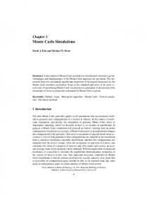
Recall that when β = 1, wn = 1 and w0 = · · · = wn−1 = 0. In this case, the first term in (20) vanishes and p0 = 1 − τ q0 (h). When 0 < β < 1, the values of unj associated with t ∈ {t0 , . . . , tn−1 } are weighted by the coefficients {w0 , w1 , . . . , wn−1 }. Figure 1 plots wm for m = 0, 1, . . . , n where n = 100 and β = 0.8. It is well-known that the sequence {wm }nm=1 are monotone increasing [6], i.e. w1 < w2 < . . . < wn−1 < wn . However, it is not true w0 < w1 . In fact, in Figure 1, w94 < w0 < w95 for both Grunwald-Letnikov and Caputo time-fractional derivative cases. is quite large relative to the other Hence, the contribution of u0j to u101 j n intermediate values of uj . We will see later on that this will have important consequences in non-Markovian random walk numerical simulations. 4. Monte Carlo protocol for the random walk 4.1. General framework. The random walk model corresponding to the governing equation in (13) uses the non-Markovian transition probabilities, wm , and the Markovian transition probabilities, pk to assign where in the ZhN lattice a particle will jump to. This jump can be based upon a

MONTE CARLO RANDOM WALK SIMULATIONS BASED . . . 359

Caputo coefficients G.L. coefficients

0

10

20

30

40

50

60

70

80

90

100

Figure 1: The weight wm associated with the density um j is plotted as a function

of m for both the Caputo and Gr¨ unwald-Letnikov (G.L.) time-fractional derivatives and β = 0.8. The lower dotted horizontal line corresponds to the value of w0 ≈ 0.005 while the upper two dotted lines correspond to wn = c1 for both the Gr¨ unwald-Letnikov (w100 = 0.8) and Caputo derivatives (w100 ≈ 0.851).

partitioning of the unit interval P = [0, 1) into two disjoint subintervals P1 and P2 such that P = P1 ∪ P2 where P1 = [0, 1 − wn ) and P2 = [1 − wn , 1). We will use a two-dimensional walk for illustration purposes. The random walk process begins by generating a uniformly distributed random number r in the unit interval and observing what subinterval (P1 or P2 ) it falls into. If r ∈ P1 = [0, 1 − wn ), then the particle will do a nonMarkovian jump, i.e. the jump will be determined by transition probabilities wm , m = 0, . . . , n − 1. Otherwise, if r ∈ P = [1 − wn , 1), then the particle will undergo a Markovian jump, i.e. the jump will be determined by transition probabilities pk . In effect, the random walk interpretation presented here is a two-dimensional extension of the one-dimensional random walk interpretation given in [11]. 4.2. Non-Markovian jumps. If 0 < β < 1 and r ∈ P1 , then the jump that the particle takes will be determined by wm , m = 0, . . . , n − 1. Let A = {A0 , A1 , . . . , An−1 } be an n-element set such that Ai = wi , i = 0, . . . , n − 1. Furthermore, let the interval P1 be refined in the following way: P1 = [B0 , B1 , . . . , Bn ), P such that B0 = 0 and Bj = j−1 i=0 Ai , j = 1, . . . , n. If r ∈ [B0 , B1 ) = [0, w0 ),

360

E. Andries, S. Umarov, S. Steinberg

then the position of the particle at t = tn+1 is given by S n+1 = S 0 (the origin). Otherwise, if r ∈ [Bj−1 , Bj ), j = 1, . . . , n, then the particle will jump back to the position that it had visited at time t = tj , i.e. S n+1 = S j . 4.3. Markovian jumps when α = 2. If r ∈ P2 = [1 − wn , 1) and α = 2 then the jump will only be to adjacent lattice grid points. Let P2 be partitioned in the following manner: P1 = [B0 , B1 , . . . , B5 ) P where B0 = 1 − wn and Bj = B0 + j−1 i=0 Ai (j = 1, . . . , 5). Here, A = {A0 , A1 , A2 , A3 , A4 } where A0 = wn − 4η and Ai = η = ντ β /hα , i = 1, 2, 3, 4. If r ∈ [B0 , B1 ), then the particle remains at the current position, otherwise if r ∈ {[B1 , B2 ), [B2 , B3 ), [B3 , B4 ), [B4 , B5 )} then the particle will move left, right, up or down, respectively, one lattice position. 4.3. Markovian jumps when DODE is given with the collection Λ = {α1 , . . . , αM }, α1 < ... < αM < 2. If r ∈ P2 = [1 − wn , 1) and Λ = {α1 , . . . , αM }, then the jump will be determined by an infinite partition refinement of P2 . Let A = {A0 , A1 , . . .}; P1 = [B0 , B1 , . . .) P such that B0 = 1−wn and Bj = B0 + j−1 i=0 Ai (j = 1, 2, . . .). In this case, the set A consists of all of the transition probabilities pk , k ∈ Z 2 , with A0 = p0 . If r ∈ [B0 , B1 ) = [1 − wn , (1 − wn ) + p0 ), then the particle will remain at the current position. Otherwise, if r ∈ [Bs , Bs+1 ), then there exists a unique k = (k1 , k2 ) ∈ Z 2 associated with s ∈ IN such that the particle will jump from S n to S n+1 = S n + (k1 h, k2 h). 5. Simulations Our motivation of the numerical simulations presented here is to see how DODE simulations of biomolecular motion of particles on a cell surface differ from those based upon the classical Brownian motion. Although the DODE random walk models are described theoretically for multivariate case in N -dimensions, nevertheless all our simulations are conducted in the two dimensional case since we are interested in the diffusion of proteins on a cell membrane surface, which can be locally approximated by a two-dimensional membrane sheet. In [12], simulated particle motion is based upon the classical Brownian motion scenario (where α = 2 and β = 1) in which the particle

MONTE CARLO RANDOM WALK SIMULATIONS BASED . . . 361 is confined within cytoskeletal barriers (see Figure 2). In these single particle tracking studies, particle appears to be spatially and temporarily confined within transient confinement zones. Although the barriers are never directly observed, it is postulated that the cytoskeletal barriers are the reason for the transient spatial confinement of particle. In principle, DODE simulations provide an alternative explanation for the observed trajectories in single particle tracking studies that does not necessarily require the existence of cytoskeletal barriers to explain transient confinement. In [12], the authors use the mean-squared-displacement formula 4aτ = h2 in which the parameters a (the diffusion coefficient) , τ (the timestep) and h (the lattice width), respectively, are given using the following values: h = 6 nanometers and τ = 1µs (microseconds, or τ = 10−6 seconds). Since the mean-squared displacement formula implicitly assumes that τβ τ p0 = 1 − 4a α = 1 − 4a = 0, h h the diffusion coefficient is then computed as a = h2 /(4τ ) = 9 × 10−12 m2 /s. To facilitate a comparison of our DODE simulations with the simulations of [12, 13], we will also use the same diffusion coefficient (a1 = · · · = aM = a = 9 × 10−12 m2 /s) and the same lattice width (h = 6 nanometers). Using the fact that the transition probabilities sum to 1, n−1 X X 1= wm + pk = (1 − wn ) + p0 + ντ β q0 (h) m=0

k

we can now solve for τ in terms of h, β, Λ and p0 , µ τ = τ (h, Λ, β, p0 ) =

c1 − p0 νq0 (h)

¶1/β

µ =

(2 − 21−β ) − p0 Γ(2 − β)q0 (h)

¶1/β .

As in [12], we set p0 = 0. However, due to the dependence of τ on Λ and β, the relative size of the timestep (from τ = 10−6 s in the case of α = 2 and β = 1) will change as Λ = {α1 , ..., αM } and β vary. Instead of fixing the simulations to have the same stepsize τ , we will fix the duration of the overall walk to be the same. Let T denote the overall duration of the random walk 1 simulation. In all of our DODE simulations, T is set to T = 30 seconds. This is equivalent to 1 frame at video rate where video rate is measured as 30 frames per second. Figure 3 shows various Markovian DODE simulations (β = 1) across various values of components of Λ. The left, middle and right plots in the top row show DODE simulations with the single term α = {2}, α = {1.5}

362

E. Andries, S. Umarov, S. Steinberg

231 165 99 33 −33 −99 −165 −231 −297 −363 −429 −495 −561 −627 −693 −759 −825 −891 −957 −1023 −1089 −1155 −1221 −561 −495 −429 −363 −297 −231 −165 −99

−33

33

99

165

231

297

363

429

495

Figure 2: This random walk simulation depicts classical Brownian motion confined to rectangular cytosketetal barriers. The parameters used in this simulation are as follows: h = 6 nanometers, τ = 10−6 s and a = 9 × 10−12 m2 /s. The barriers are spaced out every 66 nanometers and the the probability of escape is p = 0.01 when a particle encounters a barrier. and with two-terms with Λ = {1.5, 2}, respectively. The first two DODE simulations are actually monofractal DODE simulations with M = 1 while the last one (Λ = {1.5, 2}) is a multi-fractal case with M = 2. The large white dots indicate the first and last positions of the random walk and the starting position is always the origin (0, 0). It is clear that for these DODE simulations with α 6= {2} that the particle travels much longer distances since the probability of jumping to faraway lattice sites is greater than what would be expected for α = 2. Figure 4 shows various non-Markovian DODE simulations (β = 0.999) using the same values of α as in Figure 3. The bottom plot in both Figures 3 and 4 show the plots on top row superimposed on one graph. The dark shaded lines correspond to Markovian jumps (r ∈ P1 ) while the white lines correspond to non-Markovian jumps (r ∈ P2 ). The frequency of the nonMarkovian jumps are given by the size of the P1 interval. For β = 0.999, P1 ≈ [0, 1 − wn ) = [0, 0.00069339). Hence, the probability at every timestep of doing a non-Markovian jump is 0.00069339. The bottom plot in Figure 4 shows the superposition of all three non-Markovian DODE simulations on the same graph.

MONTE CARLO RANDOM WALK SIMULATIONS BASED . . . 363 For Figure 5, we have non-Markovian DODE simulations for a fixed set of α values (Λ = {0.8, 1.3, 1.8}) with β varying. The left, middle and right plots correspond to β = 0.999, β = 0.99 and β = 0.9, respectively. The probability of taking a non-Markovian per timestep for these graphs is 0.00069339 (left), 0.0070 (middle) and 0.0718 (right). For example, roughly 7% of all jumps for the right subplot on the top row are non-Markovian jumps. The effect of decreasing β is clear: the overall distances that the particle traverses is decreased since motion is constrained by jumps to previously visited positions. The average jump sizes associated with Figures 3, 4 and 5 are shown in Table 1. The numbers in the brackets before the colon correspond to the (Λ, β) pair used in the DODE simulation while the number after the colon corresponds to the average jump size. For the non-Markovian walks, the average jump length is larger when, for a fixed set of α values, β is decreased from 1. This is a consequence of the non-Markovian nature of the random walks for 0 < β < 1. Since the particle is allowed to jump back to any previously visited position, the jump size can be quite large if the previously visited position was spatially remote from the particle’s current position (see Figure 5). In particular, in Figure 1, the probability of the particle to jump back to the origin is disproportionately larger than for other previously visited sites. In Figures 4 and 5, one can observe evidence of this phenomenon. Left Plot

Middle Plot

Right Plot

Figure 3

(2,1): 6.0000

(1.5,1): 10.9770

({.5,2},1): 7.3320

Figure 4

(2,0.999): 6.0038

(1.5,0.999): 11.0707

({1.5,2},0.999): 7.3593

Figure 5

({0.8,1.3,1.8},0.999): 17.0328

({0.8,1.3,1.8},0.99): 17.1663

({0.8,1.3,1.8},0.9): 19.8946

Table 1: This table reports the average jump size (after the colon) for all of the DODE simulations in Figures 3, 4 and 5. The numbers before the colon indicates values of the (Λ, β)-pair used in the DODE simulation. 6. Conclusion In this paper we constructed the random walk simulation model based on the so called distributed order differential equations. Analyzing the obtained results and comparing them with the classic Brownian motion and other simulations based on the one-term (monofractal) fractional order differential equations, we can make the following conclusion. Qualitatively,

364

E. Andries, S. Umarov, S. Steinberg

the DODE simulations provide a richer repertoire of motion, compared to monofractal walks when M = 1. We remark that numerically this model corresponds to the explicit scheme (19), which can be considered as a generalization of the classic finite difference schemes. The obtained schemes are stable under some conditions, which we are going to report in another paper. One of the features of the represented model is that, macroscopically, the DODE trajectories tend to cluster together more often than the monofractal walks. The clustering is even more pronounced when the motion is non-Markovian due to the memory the particle has for previously visited positions. Moreover, one does not have to hypothesize the existence of barriers to explain why a particle appears trapped in a transient confinement zone or hops large distances. The clustering of trajectories and large jumps are a natural consequence of the DODE random walk model. However, when the motion is non-Markovian, the particle has a strong propensity to jump back to the origin, a consequence of the disproportionately large weight w0 associated with u0j . While jumping back to previously visited ’compartments’ is observed for experimentally observed single particle tracking data [13], one does not experimentally observe molecules jumping back from its current position to the starting point. Nonetheless, the DODE random walk models closely resemble the data from single particle tracking experiments of molecules moving on cell membranes [12, 13]. This is not surprising since the motion of biomolecules on the cell surface occurs in a very heterogeneous environment. Acknowledgment. This paper is partially supported by NIH grant P20 GMO67594. References [1] R.L. Bagley, P.J. Torvic, On the existence of the order domain and the solution of distributed order equations I, II. Int. J. Appl. Math. 2 (2000), 865-882, 965-987. [2] J. Bouchaud, A. Georges, Anomalous diffusion in disordered media: Statistical mechanisms, models and physical applications. Physics Reports 195 (1990), 127-293. [3] M. Caputo, Linear models of dissipation whose Q is almost frequency independent. II. Geophys. J. R. Astr. Soc., 13 (1967), 529-539. [4] M. Caputo, Distributed order differential equations modeling dielectric induction and diffusion. Fract. Calc. Appl. Anal. 4 (2001), 421442.

MONTE CARLO RANDOM WALK SIMULATIONS BASED . . . 365 [5] A.V. Chechkin, R. Gorenflo, I.M. Sokolov, V. Gonchar, Distributed order time fractional diffusion equation. Fract. Calc. Appl. Anal. 6 (2003), 259-279. [6] M. Ciesielski and J. Leszczynski, Numerical simulations of anomalous diffusion. In: Computer Methods in Mechanics, June 3-6, 2003, Gliwice, Poland. [7] K. Diethelm, N.J. Ford, Numerical solution methods for distributed order differential equations. Fract. Calc. Appl. Anal. 4 (2001), 531542. [8] M. Edidin, Lipid microdomains in cell surface membranes. Curr. Opin. Struct. Biol. 7 (1997), 528-532. [9] R.N. Ghosh, W.W. Webb, Automated detection and tracking of individual and clustered cell surface low density lipoprotein receptor molecules. Biophys. J. 66 (1994), 1301-1318. [10] R. Gorenflo, Yu. Luchko, S. Umarov, On the Cauchy and multipoint problems for partial pseudo-differential equations of fractional order. Fract. Calc. Appl. Anal. 3, No 3 (2000), 249-277. [11] R. Gorenflo, F. Mainardi, D. Moretti, G. Pagnini and P. Paradisi, Discrete random walk models for space-time fractional diffusion. Chemical Physics 84 (2002), 521-541. [12] K. Ritchie, X.-Y. Shan, J. Kondo, K. Iwasawa, T. Fujiwara, A. Kusumi, Detection of non-Brownian diffusion in the cell membrane in single molecule tracking. Biophys. J. 88 (2005), 2266-2277. [13] K. Suzuki, K. Ritchie, E. Kajikawa, T. Fujiwara, A. Kusumi, Rapid Hop diffusion of a G-protein-coupled receptor in the plasma membrane as revealed by single-molecule techniques. Biophys. J. 88 (2005), 3659-3680. [14] F. Liu, S. Shen, V.Anh, I. Turner, Analysis of a discrete nonMarkovian random walk approximation for the time fractional diffusion equation. ANZIAM J. 46 (2005), C488-C504. [15] C.F. Lorenzo, T.T. Hartley, Variable order and distributed order fractional operators. Nonlinear Dynamics, 29 (2002), 57-98. [16] M. Meerschaert, P. Scheffler, Limit theorems for continuous time random walks with slowly varying waiting times, Statistics and Probability Letters 71, No 1 (2005), 15-22. [17] M. Meerschaert, P. Scheffler, Limit Distributions for Sums of Independent Random Vectors. Heavy Tails in Theory and Practice. John Wiley and Sons, Inc, New York (2001).

366

E. Andries, S. Umarov, S. Steinberg

[18] R. Metzler, J. Klafter, The random walk’s guide to anomalous diffusion: a fractional dynamics approach. Physics Reports 339 (2000), 1-77. [19] S.G. Samko, A.A. Kilbas, O.I. Marichev, Fractional Integrals and Derivatives: Theory and Applications. Gordon and Breach Science Publishers, New York and London (1993). [20] M. Saxton, Anomalous Subdiffusion in Fluorescence Photobleaching Recovery: A Monte Carlo Study. Biophys. J., 81, No 4 (2001), 22262240. [21] M.J. Saxton, K. Jacobson, Single-particle tracking: applications to membrane dynamics. Ann. Rev. Biophys. Biomol. Struct., 26 (1997), 373-399. [22] V.V. Uchaykin, V.M. Zolotarev, Chance and Stability. Stable Distributions and their Applications, VSP, Utrecht (1999). [23] S. Umarov, R. Gorenflo, On multi-dimensional symmetric random walk models approximating fractional diffusion processes. Fract. Calc. Appl. Anal. 8 (2005), 73-88. [24] S. Umarov, R. Gorenflo, The Cauchy and multipoint problem for distributed order fractional differential equations. ZAA 24 (2005), 449-466. [25] S. Umarov, S. Steinberg, Random walk models associated with distributed fractional order differential equations. In: High Dimensional Probability, IMS Lecture Notes - Monograph Ser. 51 (2006), 117-127. [26] G. Zaslavsky, Chaos, fractional kinetics, and anomalous transport. Physics Reports 371 (2002), 461-580. †

Department of Mathematics and Statistics The University of New Mexico 1 University of New Mexico, MSC03-2150 Humanities Bldg # 81 Albuquerque, New Mexico 87131, USA

‡

Department of Pathology The University of New Mexico Albuquerque, New Mexico 87131, USA

Received: June 20, 2006

∗

Department of Mathematics and Mechanics The National University of Uzbekistan, Tashkent, UZBEKISTAN

e-mails: [email protected], [email protected], [email protected]

MONTE CARLO RANDOM WALK SIMULATIONS BASED . . . 367

300 2000

2000

100

1500

1500

0

1000

1000

−100

500

500

0

0

200

−200 −300

−500

−500 −400

−1000

−1000

−500 −400

−200

0

−1000

0

1000

−500

0

500 1000 1500

1500

1000

500

0

−500

−1500

−1000

−500

0

500

1000

1500

Figure 3: The first three subplots in the top row correspond to Markovian DODE simulations (β = 1) with different values of α: α = 2, α = 1.5 and Λ = {1.5, 2} for the left, middle and right plots. The bottom plot superimposes all of the top three simulations on one graph.

368

E. Andries, S. Umarov, S. Steinberg

2000 600

2000 1500

400 1500

1000

200

500

0

1000

0

−200

−500

−400

−1000

500

−600

−1500

−800

−2000

0 0

500

1000

−1000

−500

0

0

1000

2000

3000

2500

2000

1500

1000

500

0

−500

−1000

−1000

−500

0

500

1000

1500

2000

2500

3000

3500

Figure 4: The first three subplots in the top row correspond to non-Markovian DODE simulations (β = 0.999) with different values of α: α = 2, α = 1.5 and Λ = {1.5, 2} for the left, middle and right plots. The dark shaded lines correspond to non-Markovian walks while the white lines indicate non-Markovian jumps to previously visited positions. The bottom plot superimposes all of the top three simulations on one graph.

MONTE CARLO RANDOM WALK SIMULATIONS BASED . . . 369

4000

3000 1000

2000

3000

1000

0

0

−1000

−1000

−2000

1000

−3000

0

−4000

−1000

−2000

2000

−3000 −4000 −2000

0

2000

4000

−5000 6000 −4000

−2000

0

2000

0

2000

4000

4000

3000

2000

1000

0

−1000

−2000

−3000

−4000

−5000 −4000

−2000

0

2000

4000

6000

8000

Figure 5: The first three subplots in the top row correspond to non-Markovian DODE simulations with Λ = {0.8, 1.3, 1.8} and different values of β: β = .999, β = .99 and β = .999 for the left, middle and right plots. The dark shaded lines correspond to nonMarkovian walks while the white lines indicate non-Markovian jumps to previously visited positions. The bottom plot superimposes all of the top three simulations on one graph.