Feb 1, 2008 - been made towards answering some basic questions about knots, showing for instance that a sufficiently ..... zontal bonds; (b) perpendicular diagonal bonds; (c) bonds at 135â¦. Case of parallel ..... Thin lines indicate an arbitrary (supposedly drawn ...... In practice, we observe a value a λ1 < 3/4 and λ2 > 1/4 ...
arXiv:cond-mat/9901041v1 [cond-mat.stat-mech] 7 Jan 1999
Monte Carlo Results for Projected Self-Avoiding Polygons: A Two-dimensional Model for Knotted Polymers E. Guitter and E. Orlandini CEA-Saclay, Service de Physique Th´eorique, F-91191 Gif-sur-Yvette Cedex, France February 1, 2008
Abstract We introduce a two-dimensional lattice model for the description of knotted polymer rings. A polymer configuration is modeled by a closed polygon drawn on the square diagonal lattice, with possible crossings describing pairs of strands of polymer passing on top of each other. Each polygon configuration can be viewed as the two-dimensional projection of a particular knot. We study numerically the statistics of large polygons with a fixed knot type, using a generalization of the BFACF algorithm for self-avoiding walks. This new algorithm incorporates both the displacement of crossings and the three types of Reidemeister transformations preserving the knot topology. Its ergodicity within a fixed knot type is not proven here rigorously but strong arguments in favor of this ergodicity are given together with a tentative sketch of proof. Assuming this ergodicity, we obtain numerically the following results for the statistics of knotted polygons: In the limit of a low crossing fugacity, we find a localization along the polygon of all the primary factors forming the knot. Increasing the crossing fugacity gives rise to a transition from a self-avoiding walk to a branched polymer behavior.
1
The statistical properties of self-avoiding polymers are now very well understood, mainly thanks to the famous equivalence of the problem to a field theory, leading to a natural derivation of scaling laws and critical exponents [1]. In three dimensions however, closed polymers will generally form knots, which, for self-avoiding objects, will restrict the accessible configurations. In the last few years, some progress has been made towards answering some basic questions about knots, showing for instance that a sufficiently long polymer is knotted with probability one [2, 3], or computing the distribution of random knots [4]. However, the statistics of a closed polymer with a fixed knot-type is less well understood. Indeed, the usual field theory approach does not account for this distinction of the knot type, but corresponds rather to a summation over all the possible knot topologies. In particular, the natural question of how the critical exponents depend on the knot topology remains an open issue. Knotted configurations are encountered in the description of closed DNA molecules, with an apparent influence of the knot type on some of their properties [5]. An attempt to understand the role of a fixed knot topology was done in [6, 7, 8, 9, 10, 11] where a numerical study of knotted lattice polygons in the cubic lattice Z 3 was performed. There it was shown that, while the connectivity constant and the size exponent ν for the radius of gyration are independent of the knot type, the entropic exponent α for the number of accessible configurations clearly depends on the knot at hand. More precisely, α seems to depend only on the number of primary knots (factors) and increases by one for each added factor in the knot factorization. In practice, all the characterizations of knots involve only their projection in a two-dimensional (2D) plane. Therefore, nothing prevents us from considering a twodimensional model for knotted polymers. Such a model should be in principle much simpler to study, both analytically and numerically. The aim of this paper is precisely to introduce and study numerically a particular model of “projected” polygons on a 2D lattice, describing 2D knotted polymers. In a 2D model for knotted polymers, the self-avoiding constraint in two dimensions is released to allow for what we call “crossings”. By crossings, we actually mean two strands of the chain passing on top of each other in the projection. The object remains self-avoiding in the sense that the underlying and overlying strands cannot be exchanged by passing through each other. With this restriction, each closed polymer has a fixed knot type, which can be preserved in the deformations. Still the object is two-dimensional in the sense that its entropy corresponds to 2D deformations only. In particular, we will recover in some limits some of the usual exponents of 2D self-avoiding walks (SAW). The paper is organized as follows. In the first section, we introduce our lattice model of projected self-avoiding polygons. Section 2 describes the local elementary moves which we use to deform the polygon and explore its accessible phase space at a fixed knot topology. The issue of ergodicity is also discussed in this section where arguments for a proof of ergodicity within a fixed knot type (but not a full proof) are given. The elementary moves are then performed according to a Monte Carlo Metropolis algorithm, drawn to reproduce the most natural grand canonical statistical weight, with a fugacity K per bond of polygon, and a fugacity w per crossing. The updating rules are discussed in section 3. Several improvements of the algorithm are described in section 4. They involve both non local deformations and 2
Figure 1: An example of a PSAP configuration on the square diagonal lattice with six crossings and the topology of a trefoil knot.
multiple chains run in parallel. Our numerical results are presented in sections 5, 6 and 7 for w = 1, w → 0 and w > 1 respectively. We gather our conclusions in section 8.
1
The Model
We present here the model of Projected Self-Avoiding Polygons (PSAP’s) that we shall use to describe two-dimensional knotted polymers. The model is defined on the square diagonal lattice in two dimensions, namely the simple two dimensional square lattice Z 2 completed with the diagonals of the squares. We treat each diagonal as an elementary edge of the lattice, i.e. we consider that the intersection point of the two diagonals is not a vertex of the lattice. The bonds of the polymer can sit on all the edges of the lattice, either vertical, horizontal or diagonal, with at most one bond per lattice edge. Different rules apply for the edges and vertices of the simple square lattice on the one hand and for the diagonal edges on the other hand. We impose a strict self-avoidance at the vertices of the square lattice, i.e. we do not allow two parts of the polymer to either cross each other or even to touch each other at these vertices. We allow crossings to take place inside a square at the intersection point of its two diagonal edges. More precisely, we use the diagonal edges only for crossings, i.e. we impose that a diagonal edge can be occupied if and only if the perpendicular diagonal edge in the same square is also occupied, with the two bonds on these edges forming a crossing. For each pair of occupied diagonal edges inside a square, we distinguish between two different possible crossings according to which of the two bonds of polymer passes on top of the other. We can thus view crossings as a two dimensional projection of a pair of bonds in three dimensions, with one bond 3
I
II
III
Figure 2: The three types (I, II and III) of Reidemeister moves on the projections of knots. Reversing all the crossings also corresponds to allowed transformations.
lying on top of the other. Finally, we limit ourselves to closed polymers. Figure 1 shows an example of an allowed configuration with six crossings and the topology of a trefoil knot. Our model can be seen as a simple extension of the usual model describing selfavoiding polymer loops on the square lattice, also refered to as Self-Avoiding Polygons (SAP). The new ingredient here is the possibility for the polymer, which is strictly self-avoiding on the square lattice, to have crossings taking place on pairs of perpendicular diagonal edges inside a square. Again, these “crossings” are viewed as the two dimensional projection of two bonds of polymer passing on top of each other, with thus two distinct allowed configurations according to which of the two bonds is on top of the other. Thanks to this distinction, our model still describes a particular self-avoiding object in the sense that it mimics the projection in two dimensions of a polymer which would be self-avoiding in three dimensions. We will refer to our model as a model of Projected Self-Avoiding Polygons (PSAP’s). Since we use closed polygons, a PSAP will in general form knots, i.e. will be the two-dimensional projection of a three dimensional knot. In this sense, we can speak of our model as describing two-dimensional knotted polymers. To fully specify the model and to study the corresponding statistics, we need to assign to each PSAP configuration its weight. Since our aim is the study of knotted polymers of a fixed knot type, we want to attach a non-zero weight only to those configurations which have the desired knot-topology. We will be mainly interested below in rather simple topologies, i.e. that of the unknot (∅), that of the trefoil knot (31 ), that of the figure eight knot (41 ) and that of the composite knots made of two trefoils (31 #31 ) or a trefoil and a figure eight (31 #41 ). In practice, we will start with an initial configuration fixing the knot type and we will explore the phase space accessible by performing successive transformations (moves) on the PSAP which preserve its topology. As well known from knot theory, local deformations exist on the projection of a knot which preserve its topology. These deformations are classified 4
as the Reidemeister moves [12], which are of three types as described in figure 2. These topological deformations are sufficient to pass from any two configurations of the same knot type. The set of allowed moves in our lattice model will be described in detail in the next section. For all the accessible conformations of PSAP of a given knot type, we moreover weigh the configuration by a factor π (P) =
nQ K n w c Gτ (Q, K, w)
(1)
where n is the number of bonds of the PSAP configuration P, with a fugacity K per bond, and c is the number of crossings, with a fugacity w per crossing. We also artificially introduce a factor nQ with a factor Q > 1 for numerical convenience. This factor is unimportant for averages at fixed n (canonical ensemble) but it can improve the statistics in a grand-canonical ensemble with varying n. We typically take Q = 2 in the following. The denominator in eq.(1) is the grand-canonical partition function at fixed knot-topology τ , which normalizes the weights so that the total weight for all accessible configurations is equal to unity. For the knot-topology preserving moves, the above weight will dictate the probability to accept or reject the deformation.
2
Local Elementary Moves
In this section, we describe the local part of our algorithm, which is a grand-canonical implementation, since it involves changes in the number of bonds of the projected polygon. Our algorithm uses local elementary moves of four different types depending on how many elementary squares of Z 2 (plaquettes) are involved in the move. We will use single, double, 3-plaquette (or corner) and 6-plaquette moves. We first give here a description of all these elementary moves. The way we decide in the algorithm which type of move we attempt and with which probability we accept or reject the attempted move is described in the next section. Single Moves Single Moves are performed on a single plaquette, and may involve length changes through the addition or subtraction of bonds in the PSAP. This moves are defined as follows: given a horizontal or vertical bond (pi , pi+1 ) of the current PSAP, we pick a unit vector ei perpendicular to (pi , pi+1 ). This defines a plaquette (pi , pi+1 , pi+1 + ei , pi + ei ). A move can occur only if the edge (pi + ei , pi+1 +ei ) is not occupied. The move depends on how many edges are occupied on the plaquette. If exactly two edges are occupied, we exchange occupied and unoccupied edges. This corresponds to a on bead flip (transformation SI in figure 3). If only one edge is occupied, we shift (pi , pi+1 ) one lattice spacing in the direction of ei and complete the PSAP by two additional bonds, either on the sides, creating a kink (transformation SII in figure 3), or on ′ the diagonals, creating a crossing (transformation SIV or SIV in figure 4). If exactly three edges are occupied, we move (pi , pi+1 ) to (pi + ei , pi+1 + ei ) and delete the two other bonds. The result is either a kink deletion (transformation SIII in figure 3) or a crossing deletion (transformation SV or SV′ in figure 4). 5
t
t
t
t
t
t
SI SII
t
t
t
t
� t
t
SIII
Figure 3: Single local c-preserving moves. (SI ) One-bead flip (∆n = 0). (SII ) Kink insertion (∆n = +2). (SIII ) Kink deletion (∆n = −2). SIV
t
t
t
t
� t
t
S2
SV
S4
′ SIV
� t
t
S2
SV′
t t @ @ t @t
S4
′ Figure 4: Single local c-changing moves: Reidemeister I moves. (SIV ,SIV ) Crossing ′ insertion (∆c = +1). (SV ,SV ) Crossing deletion (∆c = −1).
The single moves can be classified into two different sub-groups depending on whether they do or do not preserve the number of crossings c of the PSAP. The c-preserving moves illustrated in figure 3 are known in the literature as the BFACF moves [13, 14, 15]. While the move SI (one-bead flip) is n-preserving, the moves SII (kink insertion) and SIII (kink deletion) change the length of the PSAP respectively by ∆n = +2 and ∆n = −2. The c-changing moves are illustrated in figure 4. In this case, in addition to the change ∆n = ±2 in the length of the PSAP, the number of crossings changes by an amount ∆c = +1 ′ ′ (moves SIV and SIV ) or ∆c = −1 (moves SV and SV′ ). The moves SIV and SV′ are identical to the moves SIV and SV apart from the reversing of the crossing between S 4 and S4 . All these c-changing moves correspond to a Reidemeister I transformation. Double Moves A double move is performed on two adjacent plaquettes. Double moves are selected by first choosing, along the current PSAP, a vertex pi . Different kinds of double moves are considered, depending on the relative orientations of the two bonds (pi−1 , pi ) and (pi , pi+1 ) shared by the vertex pi (see figure 5):
6
pi−1 pi−1
pi
pi+1
t
t
t
pi+1
t @ p @ i @t
t
(b)
(a) pi+1 t
pi−1 pi t
t
(c) Figure 5: Different cases considered for double moves: (a) parallel vertical or horizontal bonds; (b) perpendicular diagonal bonds; (c) bonds at 135◦ .
Case of parallel vertical or horizontal bonds: If the two bonds are parallel, we choose one of the two possible unit vectors ei perpendicular to (pi−1 , pi+1 ), and we check if the vertex pj = pi + ei belongs to the current PSAP configuration. If it does, we look for a 2-plaquette configuration D1 such as that depicted in figure 6. If this 2-plaquette configuration is encountered, we make the local transformation DI by exchanging pi and pj = pi + ei , leading to the configuration D2 with two more crossings, or make the similar transformation DI′ leading to the reversed configuration D2 . Case of perpendicular diagonal bonds: If (pi−1 , pi ) and (pi , pi+1 ) are on perpendicular diagonal edges, the PSAP necessarily has two crossings involving two strands of polygon. We check that we have a configuration of type D2 or D2 i.e. that the two strands are not entangled (see figure 6). If ′ so, we then make the local transformation DII or DII to suppress the two crossings.
Case of bonds at 135◦: If one of the bonds, say (pi−1 , pi ) is vertical or horizontal, and the other bond (pi , pi+1 ) is at 135◦ on a diagonal edge, the procedure is analogous to the case of parallel bonds, with ei the unit vector perpendicular to (pi−1 , pi ) and inside the convex sector (pi−1 , pi , pi+1 ). After checking that the vertex pj = pi + ei belongs to the current PSAP, we look for a 2-plaquette configuration such as the one depicted in figure 7. We then let the crossing diffuse one step, according to transformation DIII of figure 7. A similar procedure is used for the configuration D 3 obtained by reversing the crossing of D3 . Finally, no double move is performed if the two consecutive bonds shared by pi belong to the same plaquette. In this case a corner move (see below) will be attempted instead. Transformations DI and DII can be though of as Reidemeister II moves while transformation DIII is simply a diffusion of the crossing to a neighboring pla7
t
t
DI
t
t -
� t
t
t
t
DII
D1
t t @ @ t @t
D2
Figure 6: Double c-changing moves : Reidemeister II moves.
t
DIII
t t @ @ t @t
t
-
t t @ @ t @t
t t
D3
Figure 7: Double c-preserving move: diffusion of a crossing.
quette. In addition to the configurations described above, there are also 2-plaquette configurations in which the two involved strands of the PSAP are consecutive. We call these configurations degenerate since can be transformed one into another by the same set of double moves above. Some of such configurations are illustrated in figure 8. Corner Moves . In these moves, three plaquettes of the underlying squared lattice are involved. As for the double moves, we first choose a vertex pi of the current PSAP. A corner move can be performed if the bonds (pi−1 , pi ) and (pi , pi+1 ), shared by the chosen vertex pi , are on the two consecutive edges of a square, as illustrated in figure 9. In this case, we check if the vertex pj = −pi + pi+1 + pi−1 . belongs to the current PSAP. If so, we look for local configurations involving three plaquettes such as those depicted in figure 10 (C1 ,C2 ) and in figure 11 (C3 ). If the local 3-plaquette configuration does not correspond to any of such configurations no move is performed. Otherwise, we attempt one of the corner moves illustrated in figures 10 and 11. We can think of the corner
t
t
DI
t
t -
� t
t
t
D1 t t
t
DII DIII
t t @ @ t @t
-
D3
t t @ @ t @t
D2 t t @ @ t @t
t t
Figure 8: Degenerate configurations for double moves. 8
pi
pi+1 t
t
t
3 pj
pi−1
Figure 9: Starting configuration for a corner move. pi
CII t
t
pi
t
t
t
t
tp
t
t
t
� t
t
t
t
pj
t
CI
C1
j
t
C2
Figure 10: Corner c-changing move: Reidemeister II move around a corner.
moves CI and CII as Reidemeister II moves, whereas the corner move of figure 11 corresponds to a diffusion of a crossing through the corner. Note that this diffusion around a corner also involves a rotation of the the crossing on the ′ square lattice. Corner moves CI′ and CII connecting configuration C1 to C 2 are also possible. In addition, as for the double moves, there are again degenerate configurations that can be transformed one into another by the same corner moves described above. Some of them are illustrated in figure 12. 6-plaquette Moves (Reidemeister III moves). This moves are performed by choosing a diagonal bond in the current PSAP. This bond singles out a crossing. We then look for the presence of two neighboring crossings along two adjacent diagonal directions, chosen at random. We finally look for configurations such as the one depicted in figure 13. The performed move RI corresponds to a Reidemeister III move. Here again degenerate configurations exist which can be changed one into another. Note that double, corner and 6-plaquette moves do not change the number n of bonds in the PSAP.
pi
pi t
t
t
t
t
t
t
t
t
t
t
-
pj
CIII
C3
t t pj @ @ t @t
t
Figure 11: Corner c-preserving move : diffusion of a crossing around a corner.
9
pi
CII t
t
pi
t
t
t
t
tp
t
t
t
� -
pi
t
t
t
t
pj
t
CI
C1
pi
t
t
t
t
t
t
t
t
j
t
C2 t
t
t
-
pj
t t pj @ @ t @t
CIII
t
C3
Figure 12: Degenerate cases of corner moves. t
t
t
t
t t @ @ t @t
t
t
t
t
t
t
t t @ @ t @t
t
t
t
t
t -
RI t
R1
Figure 13: 6-plaquette c-preserving move : Reidemeister III move.
To end this section let us mention that: • For all the moves drawn above, equivalent moves exist which are obtained by 90◦ rotations or mirror reflections. • If after our checks we do not find one of the above described environments, no move is performed. • As described in the next section we have an exhaustive procedure to decide which type of move will be attempted. All the moves above clearly preserve the knot-topology. Therefore any possible deformation will maintain the PSAP inside the set of conformations having the same knot type as the conformation one started with. In the following, we will assume that the algorithm is ergodic, although a full proof of ergodicity goes far beyond our goal. By ergodicity, we mean that starting from a given conformation, any other conformation with the same knot-topology can be obtained by a series of successive elementary moves. In the absence of crossings, our algorithm reduces to the BFACF algorithm [13, 14, 15], which is known to be ergodic. More precisely, the BFACF moves (moves SI , SII and SIII ) allow to deform any configuration of a set of selfavoiding paths onto any other configuration with the same topology and, if some of the paths are open, with the same positions of the end-points. Our algorithm completes the BFACF algorithm with knot-topology preserving moves allowing the 10
three types of Reidemeister moves, as well as the migration of a crossing along the PSAP. Although we have no rigorous proof of ergodicity for our algorithm, let us present here what could be the sketch of a proof. Before we proceed, let us note that we can limit ourselves without loss of generality to conformations on which none of the transformations SV , CII or DII (which decrease the number of crossings) can be performed. If such a transformation can be performed, then we do perform it (possibly recursively) so as to eliminate the spurious crossings. We are thus left with configurations where the suppression of a crossing requires more than one elementary move. We then divide the set of remaining conformations with a fixed knot type into subsets of conformations which have precisely the same (topologically speaking) knot projection. The topology of such a subset is characterized by a fixed number of crossings, and a fixed prescription for the connectivity of these crossings. A proof of ergodicity can then be established in two steps: • (1) Proving the ergodicity within a subset, i.e. for a fixed topology of the projection (i.e. a fixed number of crossings and a fixed set of connections between them). • (2) Showing the possibility to pass from a particular element (representative) of one subset to a particular element of another subset if the two different projections represent the same knot. Since two projections representing the same knot can be related by a series of Reidemeister moves, it is enough to prove point (2) that representatives of two different subsets differing by a Reidemeister move can be related one to the other. A good choice of representatives is what could be called expanded configurations, i.e. configurations in which all the crossings are well separated. In a grand-canonical ensemble, such configurations always exist, whatever big is the number of crossings in the projection. A Reidemeister move will involve at most three crossings in the projection. For well separated crossings, the figures 14, 15 and 16 show how to perform a Reidemeister transformation of type I, II or III respectively by use of our elementary moves. For a Reidemeister I move, we can use the BFACF moves to shrink a path with neighboring end-points onto the segment joining these end-points, then use the move SIV or SV to create or destroy a crossing, and use BFACF moves again to re-inflate the path. For Reidemeister moves II and III, the idea is to use the BFACF moves to deform the paths (with fixed end-points) connecting crossings so as to create channels along which the crossings can migrate. The migration of crossings along a channel is performed by use of the elementary moves DIII or CIII (at a corner) until the crossings come in contact and an elementary move DI or DII (Reidemeister II), or RI (Reidemeister III) can be performed. The target expanded configuration can then be reached again by creating channels, moving the crossings to their final positions, and eventually re-deforming the connecting paths. Note that for all these deformations, the moves CI and CII have not been used. This is because these moves are not independent and can be performed by a sequence of DI , DII , DIII , CIII and
11
(a) BFACF
SV
(b) BFACF
SIV
Figure 14: The passage between two expanded configurations (a) and (b) related by a Reidemeister I transformation. Thin lines indicate an arbitrary (supposedly drawn a the square lattice) path joining the crossings. For each step of the transformation, we indicate the type of elementary move involved.
(a)
BFACF
DIII CIII
DII
DI
(b) BFACF
Figure 15: The passage between two expanded configurations (a) and (b) related by a Reidemeister II transformation.
BFACF moves. Still in a Monte Carlo program, it is worth implementing them to accelerate the algorithm. Let us now come to the point (1) of our argument, i.e the ergodicity of the algorithm inside the subset of conformations having the same projection. A topological deformation will involve now only a displacement of the moves and a deformation of the paths connecting them, keeping the global connectivity structure. No Reidemeister move and in particular no creation of crossings have to be performed. Since BFACF moves allow to freely deform the already existing (i.e. with non-zero initial length) paths, and the moves DIII and CIII allow to move any crossing along a channel of connecting paths, the only possible source of blocking is due to situations where crossings have zero length connecting paths, i.e. are nearest neighbors of other
12
(a)
BFACF
DIII CIII
BFACF
RI
(b) BFACF
DIII CIII
BFACF
Figure 16: The passage between two expanded configurations (a) and (b) related by a Reidemeister III transformation.
Figure 17: A blocked configuration with a loop of 14 alternating crossings.
crossings, without path between them. Indeed, our moves do not allow us to move several crossings at once. For this situation to lead to a real blocking, one moreover needs a set of neighboring crossings whose centers form a loop on the dual square lattice (the centers of the squares), so that each crossing in the loop in blocked on both sides (see an example in figure 17). Since spurious crossings have already been removed, these loop conformations require moreover many alternating crossings (at least eight) and correspond to entangled situations with a complex knot topology. We do not expect such conformations to belong to the simple knot topologies that we study here where we consider knots made only of trefoils and figure eight primary knots.
3
Updating and Reversibility
We will now discuss the updating of our system, i.e. how we decide which type of move to attempt and with which probability we accept the move. These choices are dictated by a condition of reversibility of the algorithm and by the nature of the 13
invariant limiting distribution which we want to reach within an ergodicity class, i.e. the weight π(P) of eq.(1) which we assign to a configuration P of the PSAP. The implementation of the algorithm is “Metropolis style”. Let P1 be the current PSAP with n1 bonds and c1 crossings. A tentative move of type M is chosen according to a procedure which we describe below. It may or may not be possible. If it is, it produces a new configuration P2 with length n2 and number of crossings c2 . Then we accept the move with the acceptance rate "
n2 −n1
Acc(P1 → P2 ) = A(M) min 1, K
�
n2 n1
�Q−1 #
h
min 1, w c2−c1
i
(2)
The two min[·] terms correspond to the usual Metropolis acceptance rate dictated by the limiting distribution of eq. (1). In particular, the term involving the ratio n2 /n1 is necessary to reproduce the nQ dependence of π(P). In addition, we also introduce a coefficient A(M) ≤ 1 depending on the type of move M attempted, and which we will determine later. The probability to pass from the configuration P1 to the configuration P2 is thus "
Prob(P1 → P2 ) = A(M) min 1, K
n2 −n1
�
n2 n1
�Q−1 #
h
i
min 1, w c2−c1 × B(P1 , M) (3)
where B(P1 , M) is the probability to have selected the move M among all the tentative moves which could have been tried on P1 . To be sure that the Markov chain converges to the limiting distribution π (P), we impose on Prob(P1 → P2 ) the detailed balance condition π (P1 ) Prob{P1 → P2 } = π (P2 ) Prob{P2 → P1 } (4) This will dictate the choice of A(M) below. The implementation of the algorithm is as follows: 1. To attempt a local move on the current configuration P1 we first select with probability q a bond at random on the configuration or with probability (1 − q) a vertex at random on the configuration. The number q is a free parameter which we can adjust in our simulation. 2. Case of bond selection. In this case, after having chosen the bond at random among the n1 bonds of P1 , we attempt a 6-plaquettes move if the bond is a diagonal bond, or a single move if the bond is vertical or horizontal. (i) 6-plaquette move. Starting from the chosen diagonal bond, we look for a configuration such as those in figure 13 (or their degenerate companions). If such a configuration is not found the move is rejected. Otherwise, the outcome is a PSAP P2 with n2 = n1 and c2 = c1 , and Prob{P1 → P2 } = A(RI ) B(P1 , RI ) ; 14
B(P1 , RI ) =
2q 1 × , n1 4
(5)
The factor 2/n1 is the probability to have chosen among n1 bonds one of the two bonds forming the crossing which is the starting point of the Reidemeister III move, and the factor 1/4 is the probability to have selected the correct diagonal directions of the two other crossings involved. The important point is that every 6-plaquette move has a unique inverse (see figure 13) by design which is also a 6-plaquette move of the same type. Detailed balance holds by choosing A(RI ) = 1
(6)
since, by exchanging P1 and P2 , and using n2 = n1 , we have Prob{P2 → P1 } = Prob{P1 → P2 } and π(P1 ) = π(P2 ).
(ii) Single move. For the single moves, we proceed as described in the previous section. If the considered plaquette has two occupied edges, we do a bead flip SI . Since the bead flip SI keeps the number of bonds and crossings unchanged, the detailed balance follows by noticing that any such move has its own inverse by design. We can thus take A(SI ) = 1.
(7)
If the considered plaquette has a single occupied edge, we must choose between the three moves corresponding to an addition of two bonds (SII ,SIV ′ and SIV ) with n2 − n1 = 2 and ∆c = 0 or 1. We choose at random one of these three moves with even probability 1/3. For convenience, the ac(S) ′ ceptance rates A(SII ), A(SIV ) and A(SIV ) will be taken all equal to A+2 . To fix them, we need to consider the reverse moves, which are performed on a plaquette which has three occupied edges. In this case, the current configuration dictates without ambiguity which transformation SIII , SV or SV′ can be done. Again we take A(SIII ), A(SV ) and A(SV′ ) all equal to (S) A−2 . If P1 and P2 are the two configurations mutually exchanged by some of these transformations, with n2 = n1 + 2, we have Prob{P1 → P2 } =
(S) A+2
"
q 11 n2 min 1, K n2 −n1 n1 2 3 n1 �
�Q−1 #
h
min 1, w c2−c1
i
(8)
while Prob{P2 → P1 } =
(S) A−2
"
n1 q 1 min 1, K n1 −n2 n2 2 n2 �
Choosing (S)
A+2 = 1;
(S)
A−2 =
�Q−1 #
h
min 1, w c1−c2
1 3
i
(9)
(10)
the detailed balance Q n2 c2 n1 c1 nQ 1 K w Prob{P1 → P2 } = n2 K w Prob{P2 → P1 }
is then satisfied. 15
(11)
3. Case of vertex selection. We now suppose that we have selected a vertex, which occurs with probability (1 − q). In this case, we attempt either a double or a corner move, depending on the relative position of the two bonds (pi−1 , pi ) and (pi , pi+1 ) shared by the chosen vertex. For the relative orientations of figure 5, a double move is attempted; for the relative orientation of figure 9, a corner move is attempted. In both cases the number of bonds remains constant (∆n = 0). For the transformations DIII and CIII in which the number of crossings also remains unchanged (figure 7 and figure 11) the detailed balance holds clearly with A(DIII ) = A(CIII ) = 1 (12) by noticing that any such move has its own inverse by design. For the remaining cases (figure 6 and figure 10) the number of crossings between P1 = D1 (or respectively C1 ) and P2 = D2 or D2 (or respectively C2 or C2 ) varies by an amount c2 − c1 = 2 and we simply have to account for the fact that there are two ways to add the crossings while there is just one way to suppress them. (D,C) (D,C) Setting A(DI ) = A(CI ) = A+2 and 2A(DII ) = A(CII ) = A−2 , we have Prob{P1 → P2 } =
(D,C) A+2
×
(
2 1
)
(1 − q) × × n1
(
1 2
1
)
×
i h 1 × min 1, w 2 (13) 2
where the first line is for a double move and the second line for a corner move. The extra coefficients 2 and 1/2 in the case of a double move come respectively from the two different vertices which select the pair of parallel strands under consideration and from the probability 1/2 to make the correct choice of direction ei in which we move the vertex pi . We have conversely Prob{P2 → P1 } = The detailed balance
(D,C)
A−2 2 (D,C) A−2
×
(
2 1
)
×
i h (1 − q) × min 1, w −2 n2
Q n2 c2 n1 c1 nQ 1 K w Prob{P1 → P2 } = n2 K w Prob{P2 → P1 }
(14)
(15)
is then satisfied by choosing (D,C)
A+2
= 1;
(D,C)
A−2
1 = . 2
(16)
The analysis above may seem a little cumbersome. In practice, the only subtle point is the determination of the coefficients A(M), the list of which is displayed in Table 1. These coefficients simply correct the fact that some transformations are in competition (like a kink creation and a crossing creation) while the reverse transformation has no competitor. As usual, the Metropolis criterion simply creates the correct “energy” factor. With the above choices for the acceptance coefficients A(M), the transitions probabilities verify the detailed balance condition (4) for all PSAP’s P1 , P2 , with the invariant limit distribution of eq.(1) 16
Single Moves SI 1 SII 1 SIII 1/3 ′ SIV , SIV 1 SV , SV′ 1/3
Double Moves DI 1 DII 1/4 DIII 1
Corner Moves CI 1 CII 1/2 CIII 1
6-plaquette Moves RI 1
Table 1: Coefficients A(M) for the different local moves.
4 4.1
Improvements of the algorithm Non-local Moves
Algorithms based on local moves are known to have very long autocorrelation times which in turn lead to large statistical errors. For instance, it is known that, for the BFACF algorithm (which in our language simply corresponds to forbid crossings), the so called “exponential” autocorrelation time, which controls the relaxation of the Markov chain from an initial configuration to equilibrium, is infinite [16]. For the same algorithm, the so called “integrated” autocorrelation time, which controls the statistical error in measured quantities, is usually very large. To remedy this problem, algorithms have been proposed [6, 17] which combine local moves and non-local moves. The non-local moves correspond to select two points far apart on the chain and to reverse the part of the chain between them. In these hybrid algorithms, the non-local moves hopefully ensure the rapid equilibration within subspaces of fixed length n, while local moves ensure equilibration between different values of n. Now if one wants to study the statistics of polygons with a fixed knot type, one must make sure that the non-local moves preserve the topology of the polygon. For the usual non-local moves performed on 3-dimensional Self-Avoiding Polygons in Z 3 , this is in general not the case. One way to deal with this problem is then to check potential changes in the knot type by calculating a topological invariant such as the Alexander polynomial at every successful non-local move [6]. This is however computationally costly and it also has the disadvantage that the Alexander polynomial is not a perfect characterization of the knot type and distinct knots can have the same Alexander polynomial. The situation is different in our model where the two-dimensional character of the PSAP allows the introduction of non-local moves that do preserve the topology of the PSAP. The non-local move we consider are performed by first selecting two vertices (p1 and p2 ) in the PSAP with uniform probability. If these vertices are neighbors, no move is attempted; if not, the vertices separate the PSAP into two arcs, say a1 and a2 . If the two arcs have no crossings in common we can perform a rotation by 180◦ of the shortest one, say a1 (see figure 18). Let a′1 be the image of a1 under this rotation. If a′1 and a2 do not intersect each other, no new crossing has been generated and the move is accepted. The important feature of this move is that it does not change the 17
a ’1
a1
a2
a2
Figure 18: Non-local transformation of a PSAP. The arc a′1 is the image of a1 by a rotation of 180◦ . The arc a2 is unchanged.
1
1
1
1 2
2
2
2
Figure 19: The passage from a trefoil to its image by a rotation of 180◦ by use if local Reidemeister moves only. We indicate only the major intermediate steps.
1
2
1
2
1
2
1
2
2
1
Figure 20: The passage from a figure eight to its image by a rotation of 180◦ by use if local Reidemeister moves only. We indicate only the major intermediate steps. 18
topology of the arc a1 and therefore, since we avoid topological interaction between the arcs, it preserves the topology of the entire PSAP. To be more precise, the absence of crossings between the two arcs guarantees that the knots in a1 and those in a2 are well separated and the total knot can be viewed as the compositions of the two knots. It is known that the composition of two knots can give at most two different results according to whether their (arbitrarily fixed) orientations do or do not match in the composition. Note that our transformation reverses this matching of orientations. The result is however unique as soon as at least one of the knots is reversible (i.e. its two opposite orientations are in fact equivalent). This is the case for all the knots that we will use, which are made of trefoils (31 ) and figure eight (41 ) knots only, both of which are reversible. In practice, we can also argue that, for a trefoil (31 ) or figure eight (41 ) knot, the passage from the arc a1 to its image a′1 can be done by using Reidemeister moves which do not involve the arc a2 . This is illustrated for the trefoil knot in figure 19 and for the figure eight knot in figure 20. The non-local move described above is the simplest one that can be implemented. More sophisticated moves can be considered in which the constraint of having no crossings between a1 and a2 can be relaxed to weaker conditions. We however limited ourself to the simplest non-local moves without crossings. In our algorithm, we therefore have an additional free parameter 0 ≤ p < 1 which is the probability that we attempt non-local move rather than a local move.
4.2
Multiple Markov Chain Method
Another way to improve the slow convergence of the local algorithm is by sampling along a set of several Markov chains run in parallel. This method, refered to as the Multiple Markov Chain (MMC) method, has been introduced by Geyer [18] and then adapted to interacting self-avoiding walks with fixed length by Tesi et al [19] (see also [20] for a more detailed analysis of the method). We describe here a variant of this approach suitable for simulations in the grand canonical (n varying) ensemble. The starting point is the single Markov chain whose limiting distribution π(P) depends on the step and crossing fugacities K and w. Here we will consider a procedure with a fixed value of w, hence the w dependence will be omitted in this section. For values of K close to (and below) the critical value Kc where the average length of the PSAP diverges, the Markov chain samples configurations with very large values of n and the convergence of the algorithm is therefore very slow. On the contrary for a value K ′ of the step fugacity such that K ′ nmin the relation pn = µn nα−3 (1 + a/n)
(24)
holds, where a is a free parameter that we can vary to mimic a correction to scaling. By varying nmin and a we can probe the sensitivity of our estimates to scaling. We generally find a region of minimum sensitivity from which we extract the following estimates: µ(∅) = 3.254 ± 0.005, 23
µ(31 ) µ(41 ) µ(31 #31 ) µ(31 #41 )
3.251 ± 0.07, 3.253 ± 0.09, 3.245 ± 0.10, 3.255 ± 0.11.
= = = =
(25)
and for the entropic exponents: α(∅) α(31 ) α(41 ) α(31 #31 ) α(31 #41 )
0.58 ± 0.03, 1.86 ± 0.06, 1.95 ± 0.08, 4.20 ± 0.15, 3.90 ± 0.20.
= = = = =
(26)
All these results are in agreement with the estimates (23) and (24).
5.2
The Metric Exponent ν
For the mean square radius of gyration, we assume the large n behavior hR2 (τ )in = Aν (τ )n2ν(τ )
(27)
where the average is performed over configurations with fixed n. In order to estimate ν from our data in the grand-canonical ensemble, we compute the expected value of the mean square radius of gyration, 2
hR (τ )i =
n hR
P
2
(τ )in nQ pn (τ )K n Q n n n pn (τ )K
P
(28)
Using the asymptotic forms (18) and (27), we get the following approximation for hR2 (τ )i close to the critical Kc : hR2 (τ )i ≃ h(τ ) (1 − Kµ(τ ))−2ν(τ )
(29)
or equivalently, using eq.(19), the approximation: hR2 (τ )i ≃ h′ (τ )hn(τ )i2ν(τ )
(30)
where we now have a relation between hR2 (τ )i and hn(τ )i. A log-log fit of our data to equation (30), where K takes a different value for each chain in our multiple Markov chain Monte Carlo, can be used to estimate ν for each knot type. Our best estimates are ν(∅) = 0.747 ± 0.005, ν(31 ) = 0.758 ± 0.010, ν(41 ) = 0.748 ± 0.010, ν(31 #31 ) = 0.760 ± 0.020, ν(31 #41 ) = 0.720 ± 0.040. 24
(31)
Within the stated error bars, the results above are all identical and consistent with the exact value νSAW = 3/4 [23] for self-avoiding walks or self-avoiding polygons in d = 2. This seems to indicate that although polygons in our model are not strictly selfavoiding since crossings are allowed for w = 1, the presence of these crossings limited to diagonal edges does not modify the scaling behavior of the radius of gyration.
6
Results for w 2, tend to zero. This result is consistent 26
1.0
0.8
λi
0.6
0.4
0.2
0.0 0.374
0.375
0.376
0.377
0.378
0.379
K Figure 23: Average length fraction λ1 and λ2 of the two largest arcs along the PSAP as a function of K for the trefoil (λ1 → ⋄, λ2 → 2), the composite knot 31 #31 (∇ and ∆) and the composite knot 31 #41 (• and × +). The dashed lines indicate the values 3/4 and 1/4 expected for two strictly localized knots moving freely along the PSAP.
with a localized knot which takes place over a number a bonds which is either finite, or at least growth less rapidly than n. This result of localization is corroborated by a direct visualization of a typical configuration, as shown in figure 24. Another interesting case is that of composite knots 31 #31 and 31 #41 , which have respectively cmin(31 #31 ) = 6 and cmin (31 #41 ) = 7. These knots are thus made respectively of exactly 12 and 14 arcs. We have plotted on figure 23 the proportions of the total length n occupied by the two largest arcs in both cases. Although the statistical errors are rather important when K → Kc , we see in each case that these proportions add up to one, with the proportion occupied by all the smaller arcs tending to zero. This result is consistent with a picture of the composite knot as made of two perfectly localized primary factors. The localization of the two primary knots is also directly visible on a typical configuration of the PSAP (see figure 25). If we assume that these localized factors move freely along the PSAP and interact only locally by preventing to pass through one another (which would require creating additional crossings), we should expect that the proportions tend to 3/4 and 1/4. Indeed, for two points at random drawn on a loop of size n, the largest arc between R them has average length (1/n) 0n dx max(x, n − x) = (3n/4) and the complementary arc has thus average length n/4. In practice, we observe a value a λ1 < 3/4 and λ2 > 1/4, which tends to indicate that the primary knots repel each other. This repulsion might however be a finite size effect. Indeed the deviation from the expected asymptotic values 3/4 and 1/4 is larger for the 31 #41 knot than for the 31 #31 knot 27
Figure 24: A typical configuration for the trefoil knot (31 ) at w ∼ 0. The number of bonds is n = 312. We have indicated the location of the knotted section.
as the 41 prime factor typically requires more bonds to be formed.
7
Results for w > 1
Up to now, we have studied only the case w = 1 where no fugacity is associated to the number of crossings and the case w → 0 where we have a minimal number of crossings compatible with the knot topology at hand. Although we obtained different values for the (non universal) connectivity constant µ, we found in both cases a value of ν compatible with the exact result νSAW = 3/4 in two dimensions, which suggest that these two cases are in the universality class of self-avoiding walks, and so is probably any case of the model with a value of w between 0 and 1. In this section, we will rather be interested in the behavior of the model for w > 1.
7.1
Connectivity µ
Let us first concentrate on the connectivity constant µ. If we denote by pn,c (τ ) the number of configurations of PSAP with n bonds, c crossings and the knot topology τ , we can introduce the canonical partition function pn (w, τ ) =
X
pn,c (τ )w c−cmin(τ )
(35)
c≥cmin(τ )
For w = 1, we recover the number pn (τ ) of configurations with knot-topology τ and with n bonds, irrespectively of their number of crossings. For w = 0, we recover the number p(0) n (τ ) of configurations with topology τ , number of bonds n, and with the minimal number of crossings cmin(τ ). We define µ(w, τ ) and α(w, τ ) by the large n behavior pn (w, τ ) ∼ A(w, τ )µ(w, τ )n nα(w,τ )−3 28
(36)
Figure 25: A typical configuration for the composite knot 31 #31 at w ∼ 0. We have indicated the location of the two primary knots.
In the grand canonical ensemble, we have Gτ (Q, K, w)/w cmin(τ ) =
X
pn (w, τ )K n nQ
(37)
n
hence we can again relate µ(w, τ ) to the inverse of the critical value Kc (w) of K for which hn(w, τ )i diverges. Before we present our numerical results, let us first establish a lower and an upper bound for µ(w). Lower bound for w > 1: The canonical partition function pn (w, τ ) is clearly bounded from below by the contribution w c of any acceptable configuration in the given knot-topology class. Since w > 1, we can obtain a larger lower bound by selecting a configuration with the maximum number of crossings. To obtain such a configuration, we start from any particular realization of the knot, as compact as possible. It will have, say, n0 bonds and c0 crossings. On any outermost bond, we can start to grow a linear sequence of crossings, such as the one depicted in figure 26. Note that we can arbitrarily choose any of the two possible crossings for each new crossing added in linear piece. The addition of this linear sequence clearly does not modify the topology of the knot. If n is the total number of bonds in the configuration, we get a total number of crossings equal to c0 + (n − n0 )/2 for any of the 2(n−n0 )/2 such configurations. We thus get n0
pn (w, τ ) > 2− 2 w c0 − 29
n0 −cmin (τ ) 2
n
× (2w) 2
(38)
n0 c0
n - n0 2
Figure 26: The growing of a linear sequence of crossings from a compact knot.
In the large n limit, this directly leads to the lower bound √ µ(w) ≥ 2w
(39)
Upper bound for w > 1: It is clear that any configuration with n bonds can have at most n/2 crossings, irrespectively of its knot type. We thus get for w > 1 n
This directly leads to
pn (w, τ ) < pn (τ )w 2
(40)
√ µ(w, τ ) ≤ µ1 w
(41)
From eqs.(39) and (41), we can deduce that at large w, µ(w) behaves like √ w→∞ µ(w, τ ) ∼ λ w √ with 2 ≤ λ ≤ µ1 ∼ 3.251.
(42)
To complete our analysis, we can also give lower and upper bounds on the case 0 < w < 1. In this case, it is clear that p(0) n (τ ) < pn (w, τ ) < pn (τ )
(43)
2.638 ∼ µ0 ≤ µ(w, τ ) ≤ µ1 ∼ 3.251
(44)
and therefore Figure 27 presents our results for µ(w) together with the above lower and upper bounds. At large √ w, we confirm the behavior of eq.(42) with λ ≃ 1.46 close to the lower bound 2.
7.2
The Metric Exponent ν: Branched Polymer Behavior
We have also estimated the metric exponent ν for different values of w > 1. Our best estimates are ν(w = 2) = 0.668 ± 0.008, ν(w = 3) = 0.665 ± 0.007, 30
12
10
µ(w)
8
6
4
2
0
5
10
15
20
25
30
35
40
45
50
w Figure 27: Estimate of µ as a function of the crossing fugacity w; the solid lines 1 1 correspond respectively to the curves µ = 3.251w 2 (upper bound) and µ = (2w) 2 1 (lower bound). The dashed line corresponds to the fit µ = 1.46(w 2 − 1) + 2.86.
ν(w = 4) = 0.645 ± 0.008, ν(w = 10) = 0.634 ± 0.010, ν(w = 15) = 0.630 ± 0.011, ν(w = 20) = 0.625 ± 0.012, ν(w = 30) = 0.620 ± 0.015, ν(w = 50) = 0.624 ± 0.020,
(45)
These values are plotted in figure 28, together with the values estimated for w → 0 and w = 1. Within the error bars, we distinguish two values for ν. For w ≤ 1, our data are consistent with the value νSAW = 3/4 of self-avoiding walks. For w > 1 however, our estimates are far below this value and approximately located around the value νBP ∼ 0.64 obtained for branched polymers in D = 2 [24, 25]. At large w, the branched polymer picture is corroborated by looking at a typical configuration, as the one depicted in figure 29. Such configurations are naturally selected at large w since long one-dimensional coils maximize the number of crossings and are thus energetically favored, while branching points, occuring at a finite energy cost, are favored for entropic reasons. From our data, a transition from the self-avoiding behavior to a branched polymer type statistics seems to occur at w = 1. For w < 1, crossings are penalized and play a marginal role without changing the asymptotic behavior of the polymer, which can be considered as self-avoiding. On the contrary, for w > 1, a finite density of crossings is present in a typical configuration, which degenerates into a branched polymer conformation. At the transition point w = 1, we find 31
0.80
0.75
ν(w)
0.70
0.65
0.60
0.55
0
10
20
30
40
50
w Figure 28: The exponent ν as a function of w. The dashed lines indicate the values of ν for self-avoiding walks and branched polymers.
occasionally interesting configurations showing a phase separation between a phase rich in crossings and a phase with few crossings (see figure 30). In this case, the largest of the largest value ν = νSAW is observed. Finally, let us note that a similar transition from a self-avoiding behavior to a branched polymer behavior has already been observed in an interacting two-tolerant trail model on the square lattice [26].
8
Conclusions
In this paper, we introduced a two-dimensional lattice model of Projected SelfAvoiding Polygons, describing two-dimensional knotted polymers rings with a fixed knot topology. We made a numerical study of the model using a Monte Carlo algorithm based on both local and non-local moves which preserve the knot topology of the polygon, together with a Multiple Markov Chain procedure. In the absence of a rigorous proof of the ergodicity of our algorithm within a fixed knot type, we gave strong arguments in favor of this ergodicity, together with the guidelines of a possible proof. We presented our numerical results for the connectivity constant µ and the critical exponents ν and α for various topologies and various values of the fugacity w associated to the number of crossings in the projected polygon. The connectivity µ is found to depend only on this fugacity w and not on the particular knot topology at hand. This is somewhat expected since µ typically measures a local property which is not affected by a global constraint such as fixing the knot topology. By measuring the radius of gyration of the polygon, we observe only two possible values for the exponent ν: a self-avoiding value 3/4 found at low w ≤ 1 irrespectively of the knot 32
Figure 29: A typical configuration for the unknot (∅) at w = 30.
Figure 30: A configuration for the unknot at w = 1, with n = 1250 bonds. One clearly sees two domains with very different densities of crossings, one being sparse while the other is dense.
33
type, and a large branched polymer value ≃ 0.64 found at large w > 1 for all knot topologies. Our data suggest that the transition between the two regimes occurs precisely at w = 1. Finally, at fixed w, the exponent α for the number of accessible configurations is found to depend only on the number of prime factors forming the knot. A weak w dependence is also observed. One nice feature of our two-dimensional model is the possibility to have more specific characterizations of the polygon conformations, such as the number of crossings or the arc lengths between successive crossings along the chain. This allowed us in particular to measure the typical extension of a knot inside the polygon. In the limit w → 0, we found for instance that the prime factors in a knotted polygon are localized and weakly interacting. Other applications of this model can be imagined, such as a statistics of the knot type of randomly drawn polygons. For an arbitrary polygon, the determination of the knot topology could be simply achieved in principle by imposing a very low value of w and letting the system evolve toward a configuration with a minimal number of crossings in the projection. In particular, it would be interesting to understand how the knot complexity increases with the number of monomers in the chain.
34
References [1] P. G. de Gennes, Exponents for the excluded volume problem as derived by the Wilson method Phys. Lett. A 38 (1972) 339-340. [2] D.W. Sumners and S.G. Whittington, Knots in self-avoiding walks, J. Phys. A: Math. Gen. 21 (1988), 1689-1694. [3] N. Pippenger, Knots in random walks, Discrete Applied Math. 25 (1989), 273-278. [4] V.V. Ribenkov, N.R. Cozzarelli and A.V. Vologodskii, Probability of DNA knotting and the effective diameter of the DNA double helix, Proc. Natl. Acad. Sci. U.S.A. 90 (1993), 5307-5311. [5] S.Y. Shaw and J.C. Wang, Knotting of a DNA chain during ring closure, Science 260 (1993) 533-536. [6] E. J. Janse van Rensburg and S.G. Whittington, The dimensions of knotted polygons, J. Phys. A: Math. Gen. 24 (1991), 3935-3948. [7] T. Deguchi and K. Tsurusaki, Topology of closed random polygons, J. Phys. Soc. Japan 62 (1993), 1411-1414. [8] T. Deguchi and K. Tsurusaki, Statistical study of random knotting using Vasiliev invariants, in Random Knotting and Linking ed K C Millett and D. W. Sumners (Singapore: World Scientific) (1994), 89-121. [9] S. Quake, Topological effects of knots in polymers, Phys. Rev. Lett. 73 (1994), 3317-3320. [10] E. Orlandini, M.C. Tesi, E.J. Janse van Rensburg and S.G. Whittington, Entropic exponents of lattice polygons with specified knot type, [11] E. Orlandini, M.C. Tesi, E.J. Janse van Rensburg and S.G. Whittington, Asymptotics of knotted lattice polygons, J. Phys A: Math. Gen. 31 (1998), 5953-5967. [12] For an introduction to knot theory, see for instance C.C. Adams, The Knot Book: an elementary introduction to the mathematical theory of knots, Ed. W. H. Freeman and company, New York (1994). [13] B. Berg and D. Foester, Random paths and random surfaces on a digital computer, Phys. Lett. 106B (1981), 323-326. [14] C. Aragao de Carvalho and S. Caracciolo, A new Monte Carlo approach to the critical properties of self-avoiding random walks, Journal de Physique 44 (1983), 323-331. [15] C. Aragao de Carvalho, S. Caracciolo and J. Fr¨ohlich, Polymers and g|φ|4-theory in four dimensions, Nucl. Phys. B [FS7] 215 (1983), 209-248. 35
[16] A.D. Sokal and L.E. Thomas, Exponential convergence to equilibrium for a class of random walk models, J. Stat. Phys. 54 (1989), 797-828. [17] S. Caracciolo, A. Pellissetto and A.D. Sokal, Nonlocal Monte Carlo algorithm for self-avoiding walks with fixed endpoints, J. Stat. Phys (1990), 1-53. [18] C.J. Geyer, Markov chain Monte Carlo maximum likelihood, in Computing Science and Statistics: Proceedings of the 23rd Symposium on the Interface, ed E M Keramidas (Interface Foundation) (1991), 156-163. [19] M.C. Tesi, E.J. Janse van Rensburg, E. Orlandini and S.G. Whittington, Monte Carlo study of the interacting self-avoiding walk model, J. Stat. Phys. 82 (1996), 155-181. [20] E. Orlandini, Monte Carlo study of polymer systems by Multiple Markov Chain method, IMA Proc. Work 7 (1996). [21] A. Berretti and A. Sokal, , J. Stat. Phys. 40 (1985), 1689-1694. [22] S. Caracciolo, A. Pellissetto and A.D. Sokal, Monte Carlo test of hyperscaling relation for the two-dimensional self-avoiding walk:II, J. Phys. A: Math. Gen. 23 (1990), 4509-4517. [23] B. Nienhuis, Exact critical point and critical exponents of O(n) models in two dimensions Phys. Rev. Lett. 49 (1982), 1062-1065. [24] B. Derrida and L. De Seze, Application of the phenomenological renormalization to percolation and lattice animals in dimension 2, J. Physique 43 (1982), 475-483. [25] E.J. Janse van Rensburg and N. Madras, A non-local Monte Carlo algorithm for lattice trees J. Phys. A: Math. Gen. 25 (1992) 303-333. [26] E. Orlandini, F. Seno, A.L. Stella and M.C. Tesi, Collapse from linear to branched polymer behavior, Phys. Rev. Lett. 68 (1992) 488-491, see also L. Turban, Generalised self-avoiding walk, J. Phys. A: Math. Gen. 16 (1983) L643-646.
36