Monte Carlo simulations of rigid biopolymer ... - Python Home Page

THE JOURNAL OF CHEMICAL PHYSICS 123, 124902 共2005兲

Monte Carlo simulations of rigid biopolymer growth processes Jenny Son and G. Orkoulasa兲 Department of Chemical and Biomolecular Engineering, University of California, Los Angeles, California 90095

Anatoly B. Kolomeisky Department of Chemistry, Rice University, Houston, Texas 77005

共Received 25 April 2005; accepted 11 July 2005; published online 23 September 2005兲 Rigid biopolymers, such as actin filaments, microtubules, and intermediate filaments, are vital components of the cytoskeleton and the cellular environment. Understanding biopolymer growth dynamics is essential for the description of the mechanisms and principles of cellular functions. These biopolymers are composed of N parallel protofilaments which are aligned with arbitrary but fixed relative displacements, thus giving rise to complex end structures. We have investigated rigid biopolymer growth processes by Monte Carlo simulations by taking into account the effects of such “end” properties and lateral interactions. Our simulations reproduce analytical results for the case of N = 2, which is biologically relevant for actin filaments. For the case of N = 13, which applies to microtubules, the simulations produced results qualitatively similar to the N = 2 case. The simulation results indicate that polymerization events are evenly distributed among the N protofilaments, which imply that both end-structure effects and lateral interactions are significant. The effect of different splittings in activation energy has been investigated for the case of N = 2. The effects of activation energy coefficients on the specific polymerization and depolymerization processes were found to be unsubstantial. By expanding the model, we have also obtained a force-velocity relationship of microtubules as observed in experiments. In addition, a range of lateral free-energy parameters was found that yields growth velocities in accordance with experimental observations and previous simulation estimates for the case of N = 13. © 2005 American Institute of Physics. 关DOI: 10.1063/1.2013248兴 I. INTRODUCTION

Rigid biopolymers are vital components of the cytoskeleton and the cellular environment. Microtubules, actin filaments, and intermediate filaments are such rigid biopolymers that play a fundamental role in biological systems by facilitating cellular transport, cell motility, and reproduction.1,2 These cytoskeletal biopolymers polymerize and depolymerize, and also move within the cytoplasm.1,2 Polymerization and depolymerization processes display the phenomenon of recurrent growing and shrinking phases which alternate stochastically. This is termed “dynamic instability” and it enables the growing microtubules to explore space and reorganize.3 Although the behavior of microtubules in living cells can be attributed to dynamic instabilities, the exact mechanisms and biological functions are not completely known. Microtubules are rigid, cylindrical tubes with diameter of approximately 25 nm that are composed of N parallel protofilaments. N varies from 10–15, but typically N = 13 is most prevalent for the ones that are nucleated from centrosomes.4 Polymerization and depolymerization dynamics of microtubules have been studied extensively, both experimentally and theoretically. Experimental measurements of growth dynamics of actin filaments and microtubules under external forces have been made,5–7 and theoretical moda兲

Electronic mail: [email protected]

0021-9606/2005/123共12兲/124902/7/$22.50

els, such as polymer ratchet8,9 and phenomenological10,11 models, have been proposed. Despite the fact that the theoretical models provide adequate descriptions of the dynamics of growing rigid biopolymers, they lack information on microscopic structure, geometrical properties of a biopolymer’s lattice, and lateral interactions between protofilaments.12,13 Computer simulations have also been employed for the study of microtubule dynamics.14 These simulations do not describe accurately the geometry of the growing ends in microtubules. Stukalin and Kolomeisky12 developed a model which takes into account the complex structure of the growing end of the biopolymer and obtained analytical solutions for the case of N = 2, which is relevant to actin filaments. In Ref. 12, two models for microtubule growth were considered, “onelayer” and “full” model, respectively. In the one-layer model, the distances between the tips of the protofilaments are constrained to lie within one subunit length in the allowed polymer configurations. In contrast, the full model has no such restriction. Despite the fact that the one-layer model is soluble15 for arbitrary N, analytical solutions cannot be obtained for the cases of N = 10– 15, which are relevant to microtubules, for the full model. Analytical difficulties arise due to the enormous number of configurations associated with N ⬎ 2. The objective of this work is to perform Monte Carlo simulations to obtain results for the growth velocities for the analytically insoluble cases of N ⬎ 2 full model in

123, 124902-1

© 2005 American Institute of Physics

Downloaded 10 Nov 2005 to 128.42.240.135. Redistribution subject to AIP license or copyright, see http://jcp.aip.org/jcp/copyright.jsp

124902-2

J. Chem. Phys. 123, 124902 共2005兲

Son, Orkoulas, and Kolomeisky

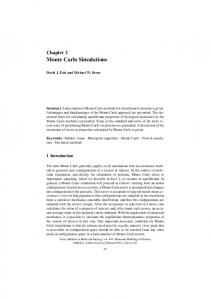
FIG. 1. Matrix diagram. 共a兲 The tip of the microtubule is flat. 共b兲 The tip of the microtubule shows jagged edges.

order to test how well the one-layer approximation describes the growth of rigid biopolymers, as well as to study the effects of activation energy coefficients for specific polymerization/depolymerization processes. For the case in which the activation energy coefficients are nonzero, the models considered in Ref. 12 cannot be solved analytically. Furthermore, for the N = 13 full model, we have found a range of lateral energy parameters that yields growth velocities consistent with experimental observations5 and previous simulations.14 In addition, since growing microtubules are known to generate forces,2,3,5 we have obtained a forcevelocity curve which is in good accord with experimental measurements5 for the analytically intractable N = 13 full model. The difference between our work and previous simulations is that we incorporated the shift distance a between adjacent protofilaments in order to explicitly calculate the magnitude of lateral interactions, whereas previous work did not focus on these microscopic details. II. DESCRIPTION OF THE MODEL

The parallel protofilaments of microtubules are polymers and their building blocks are globular proteins called tubulin subunits. Tubulin subunits are heterodimers that are composed of alternating ␣- and ␤-tubulin monomers, see Fig. 1共b兲. Because of the head-to-tail arrangement of the ␣- and ␤-tubulin subunits in protofilaments, polarity arises and the 共⫹兲– end displays a faster rate of growth than the 共⫺兲– end. In this work, we consider microtubule growth from the 共⫹兲– end only. However, the method of assembly at both ends are analogous, and recently, growth dynamics of rigid twostranded polymers at both ends has been described as a combination of growth processes at each end separately.16 Whereas previous Monte Carlo simulations on microtubule growth dynamics did not take into account the jagged edges of the growing end of the biopolymer,14 the present

work incorporates the detailed microscopic structure in the model, see Fig. 1. Note the omission of the jagged growing end of the microtubule in Fig. 1共a兲. In this schematic, the “surface” of the microtubule tip is flat, whereas in reality, it displays some “surface roughness.” In contrast, note the details of the rough edges in Fig. 1共b兲. The length of the tubulin subunit is d = 8.2 nm, and a is the shifted distance for adjacent protofilaments. Figure 1共b兲 is a much more realistic representation of a microtubule of a B-type lattice with a seam.2 Note that each rectangular tubulin subunit represents a dimer of alternating ␣- and ␤- monomers. Specific to this diagram, the Nth protofilament is termed the “leading” protofilament because it is the longest. The hollow, cylindrical nature of microtubule is simulated by mimicking a contact between the first and last columns 共protofilament 1 and N兲, see Fig. 1. Adjacent protofilaments are shifted by an arbitrary distance a. For real microtubules with N = 13, a = 0.96 nm. However, in the simplified symmetric case where seam effects are not explicitly taken into account, a can be estimated as d / 13 or a = 0.63 nm. The jagged tip of the growing biopolymer can be treated as a surface, where structural roughness arises from attachment or detachment of individual subunits.17 A variable M i is introduced as a measure of the exposed surface and molecular roughness. It represents the lateral interactions that an incoming subunit will have with its adjacent protofilaments. We explicitly calculate 关M 1 , M 2 , . . . , M i , . . . , M N−1 , M N兴 for each ith protofilament. In essence, M i are the sums of the differences in lengths 共xi兲 of protofilaments that are on either side of protofilament i, i.e., M i = 兩xi−1 − xi兩 + 兩xi − xi+1兩

共1兲

and mi =

Mi , d

共2兲

where Eq. 共2兲 represents the fraction of lateral interactions that an incoming subunit will have.18 It is known that microtubule assembly is not diffusionlimited when the tubulin subunits approach the growing biopolymer.19 Therefore, it follows that a careful investigation of the rates of attachment 共rai兲 and detachment 共rdi兲, which are in turn influenced by the complex structure of the growing end, the geometrical properties, and the lateral interactions between the protofilaments, is necessary in order to evaluate the long-time mean velocity. These rates are related by the following thermodynamic expression:12 rai/c = e−共g␷+gim+ghi兲/kBT , rdi

共3兲

where c = 25 ␮M is the concentration of free tubulin subunits used in experiments.5 Note that the appearance of c arises because the rate of attachment is proportional to the concentration of free subunits. In Eq. 共3兲, g␷ is the vertical bond energy, gim is the energy for immobilizing tubulin subunits into the rigid lattice, and ghi is the lateral bond energy. Note that these energies are negative, which is an implication of weak chemical bonds 共microtubules are noncovalent

Downloaded 10 Nov 2005 to 128.42.240.135. Redistribution subject to AIP license or copyright, see http://jcp.aip.org/jcp/copyright.jsp

124902-3

J. Chem. Phys. 123, 124902 共2005兲

Simulations of rigid biopolymer growth processes

polymers2兲. The head-to-tail binding 共vertical兲 and immobilization energies are constant for any configuration, whereas the lateral energy varies depending on the local configuration at the tip of the growing microtubule. Then the lateral energy for the ith protofilament is expressed by the following: ghi = migho ,

共4兲

where gho is a constant and mi is the measure of the fraction of lateral interactions for site i. Subsequently, the rates of attachment and detachment can be written as follows: rai ⬀ e−␪共g␷+gim+ghi兲/kBT ,

共5兲

rdi ⬀ e−共␪−1兲共g␷+gim+ghi兲/kBT .

共6兲

In Eqs. 共5兲 and 共6兲, ␪ reflects the value of the activation barrier for subunit binding, 0 ⬍ ␪ ⬍ 1.12 Attachment and detachment rates for the leading protofilament 共Ra and Rd, respectively兲 have no dependence on ghi, and they can be represented by the following expressions for any configuration:12 Ra/c = e−共g␷+gim兲/kBT . Rd

共7兲

Then rates rai and rdi for protofilaments other than the leading one can be expressed by the following: rai Ra m = ␥ i, rdi Rd

共8兲

where

␥ = e−gho/kBT

共9兲

is the lateral energy parameter. The thermodynamic expression in Eq. 共8兲 can be rewritten in the following form: rai = Ra␥ f i+共1/2兲mi ,

共10兲

rdi = Rd␥ f i−共1/2兲mi .

共11兲

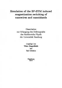
FIG. 2. 共a兲 One-layer model of the rigid polymer. 共b兲 Full model of the rigid polymer.

to the protofilament where a stronger lateral bond is created, and conversely, a slower dissociation where a stronger lateral bond is to be broken, it is necessary to investigate the degree of significance of their effects on the growth velocities of the microtubules. In Ref. 12 two different models of growth were proposed: the one-layer model and the full model. Consider a growing rigid polymer in Fig. 2. The location of the leading protofilament 共the longest protofilament兲 is where ai = 0. Using this as a reference, the one-layer model corresponds to ai ⬍ d for protofilaments other than the leading one, see Fig. 2共a兲. The absence of the constraint ai ⬍ d corresponds to the so-called full model, see Fig. 2共b兲. The ratio of the velocities of these two models are obtained in order to determine how well the simple one-layer model describes the more realistic full model. III. SIMULATION METHODOLOGY

The coefficients f i reflect the different values of activation energies for specific polymerization and depolymerization processes. In this work we first consider the case f i = 0 for the purpose of comparing our results to those of analytical results. After successful reproduction of the analytical results, f i will be explicitly determined for each protofilament under the following criteria:12 − 21 mi ⬍ f i ⬍ 21 mi

共12兲

− 1 ⬍ f i ⬍ 1.

共13兲

or

Equation 共12兲 applies to protofilaments for which the tips are at a distance less than d from the adjacent protofilaments,20 and Eq. 共13兲 applies to protofilaments for which the tips are at a distance greater than d from the adjacent protofilaments. The coefficients f i are related to the amount of lateral interactions that the incoming subunits will have based on the configurations of their adjacent protofilaments 关Eqs. 共12兲 and 共13兲兴. Since these coefficients imply a faster attachment

The growth of microtubules is a nonequilibrium process and it is thus simulated by a kinetic Monte Carlo method. Kinetic Monte Carlo algorithms are based on a dynamic interpretation of the Monte Carlo method through the master equation.21–24 They were developed to address the questions of convergence and accuracy of the Monte Carlo method22 and they also formed the basis for applying the Monte Carlo method to simulate dynamic processes.25 In this work, the growth of microtubules is simulated by a kinetic Monte Carlo algorithm that was developed for Ising systems with nearest-neighbor interactions23 and extended in stochastic formulations of chemical reactions26–28 by Gillespie. The transient behavior of a system that executes a random walk over a discrete set of states 兵S1 , S2 , . . . , Sm , . . . , Sn , . . . 其 is described by the master equation: dP共n兲共t兲 = 兺 P共m兲共t兲 · Wmn − 兺 P共n兲共t兲 · Wnm ˙ , dt m m

共14兲

where P共n兲共t兲 is the probability that the system is in state Sn at time t and Wmn is the transition probability per unit time from state Sm to Sn. Even for cases for which the transition probabilities do not have explicit time dependence 共as it is

Downloaded 10 Nov 2005 to 128.42.240.135. Redistribution subject to AIP license or copyright, see http://jcp.aip.org/jcp/copyright.jsp

124902-4

J. Chem. Phys. 123, 124902 共2005兲

Son, Orkoulas, and Kolomeisky

the case in this work兲, the master equation Eq. 共14兲 is analytically and numerically intractable. An equivalent description of the random walk, well-suited for numerical implementations, may be formulated through the transition probability density function Pn共␶ 兩 m , t兲.27 Given that the system is at state Sm at time t, Pn共␶ 兩 m , t兲d␶ is the probability that the system “hops” to state Sn in the time interval 共t + ␶ , t + ␶ + d␶兲. Pn共␶ 兩 m , t兲 is written as27 Pn共␶兩m,t兲d␶ = ˜P0共␶兩m,t兲 · Wmnd␶ ,

共15兲

where ˜P0共␶ 兩 m , t兲 is the probability that no transition occurs in the time interval 共t , t + ␶兲 共i.e., the system stays in state Sm兲 and Wmnd␶ is the probability that the system moves from Sm to Sn in the time interval 共t + ␶ , t + ␶ + d␶兲. The waiting-time probability ˜P0共␶ 兩 m , t兲 satisfies the following identity: ˜P 共␶ + d␶兩m,t兲 = ˜P 共␶兩m,t兲 · 共1 − W d␶兲, 0 0 m

共16兲

variable functions, ˜P1共␶ 兩 m , t兲 and ␲mn, respectively, see Eq. 共21兲. First, a state Sn or equivalently an integer n is selected with probability ␲mn. Let n

Fm共n兲 = 兺 ␲mj

be the probability that k 艋 n, where k is the number of several independent paths stemming from state Sm.26 If ␰1 is a random number uniformly distributed in 关0, 1兲, then integer n 共and state Sn兲 is selected if the following inequality is satisfied:29,30 Fm共n − 1兲 艋 ␰1 ⬍ Fm共n兲.

Wm = 兺 Wmn ,

共17兲

n

and Wmd␶ is the probability that the system moves away from state Sm within d␶. Rearrangement of Eq. 共16兲 yields ˜ 共␶兩m,t兲 dP 0 = − W md ␶ , ˜P 共␶兩m,t兲

共18兲

0

which can be integrated subject to ˜P0共0 兩 m , t兲 = 1 to give ˜P 共␶兩m,t兲 = e−Wm␶ . 0

共19兲

Using Eqs. 共15兲 and 共19兲, the transition probability density Pn共␶ 兩 m , t兲 can be explicitly written as Pn共␶兩m,t兲 = Wmne−Wm␶ .

共20兲

For continuous-time/discrete-state random walks, it is more convenient to express Pn共␶ 兩 m , t兲 in the following form:27 Pn共␶兩m,t兲d␶ = ˜P1共␶兩m,t兲d␶ · ␲mn ,

共21兲

where ˜P1共␶ 兩 m , t兲d␶ is the probability that a transition from state Sm to another state 共any one兲 occurs in 共t + ␶ , t + ␶ + d␶兲 and ␲mn is the “hopping” probability from Sm to Sn. ˜P 共␶ 兩 m , t兲 and ␲ are given by 1 mn ˜P 共␶兩m,t兲 = 兺 P 共␶兩m,t兲 = W e−Wm␶ , 1 n m

共22兲

n

␲mn =

Pn共␶兩m,t兲 Wmn . = ˜P 共␶兩m,t兲 Wm

共23兲

1

In the implementation of the random walk under consideration, given that the system is at state Sm at time t, one must determine at what time t + ␶ the next step occurs and to which state Sn the system jumps. The specification of the time increment ␶ and the state Sn 共or the integer n兲 is done according to the transition probability density function Pn共␶ 兩 m , t兲 and it is based on the fact that the two-variable function Pn共␶ 兩 m , t兲 can be written as the product of two one-

共25兲

A time increment ␶ must also be generated from the probability density ˜P1共␶ 兩 m , t兲. To this end, consider the probability distribution ˜F1共␶ 兩 m , t兲 defined by ˜F 共␶兩m,t兲 = 1

where

共24兲

j=1

冕

␶

d␩ ˜P1共␩兩m,t兲 = 1 − e−Wm␶ .

共26兲

0

If ␰2 is a random number uniformly distributed in 关0, 1兲, ␶ is found from ˜F1共␶ 兩 m , t兲 = ␰2 or

␶=−

1 ln共1 − ␰2兲, Wm

共27兲

which ensures that ␶ is distributed according to the probability density ˜P1共␶ 兩 m , t兲. Statistical averages are obtained by performing several independent realizations of the random walk according to the previous methodology. In the microtubule growth problem, a state Sm is characterized by a given arrangement of the protofilaments and a new state is obtained by adding or removing a tubulin subunit. If N is the number of protofilaments, the total number of states within reach of the current state is 2N.31 The 2N hopping probabilities ␲mn are defined by

␲mn =

rn

兺 j=1 r j 2N

,

共28兲

where rn is either the rate of attachment or detachment 共rai or rdi 关Eq. 共10兲 or 共11兲兴, respectively兲 of a tubulin monomer to a given protofilament. IV. RESULTS AND DISCUSSION

We have performed Monte Carlo simulations for the cases of N = 2 and N = 13 for both models, one-layer and full, respectively. In the simulations we evaluate the asymptotic 共long-time兲 mean growth velocity 具x共t兲典 ⬇ Vt,

共29兲

where x共t兲 represents the length of the biopolymer at time t. This length is the maximum value among the N protofilaments at time t in order to be consistent with the methods of experimental measurements. Our first goal is to reproduce the velocities obtained in Ref. 12 with zero activation energy coefficients f i for N = 2. The growth velocity of the microtubule is determined by calculating the statistical average 具x共t兲典 as a function of time, see Fig. 7 below. Our results are shown

Downloaded 10 Nov 2005 to 128.42.240.135. Redistribution subject to AIP license or copyright, see http://jcp.aip.org/jcp/copyright.jsp

124902-5

Simulations of rigid biopolymer growth processes

FIG. 3. Ratio of mean growth velocities V共one-layer兲 / V共full兲 for the cases of N = 2 and N = 13 as functions of the lateral energy parameter ␥. 共䊊兲 shows simulation results for N = 2, a / d = 0.6, and 共쎲兲 shows simulation results for N = 2, a / d = 0.1. The solid lines are the analytical predictions of Ref. 12 for corresponding values of a / d. 共䉱兲 shows points for N = 13, a / d = 0.1, and 共䉮兲 shows points for N = 13, a / d = 0.6. The trend for N = 13 is similar to N = 2 model.

in Fig. 3 and are compared with the analytical predictions of Ref. 12. Figure 3 shows that the simulations reproduce the analytical results consistently. Note that the larger protofilament shift distance 共a / d = 0.6兲 results in better agreement for the one-layer and the full model. This is so because more favorable lateral bonds are created for a / d = 0.6, due to the fact that more contact length is created between the incoming tubulin subunit and the protofilaments that are adjacent to the site of event. The ratio of mean growth velocities for the case of N = 13 is expected to display characteristics similar to the N = 2 case. Results for the growth velocities for N = 13 are shown in Fig. 3. The mean growth velocity ratio at ␥ = 1 is 0.907 for both a / d = 0.1 and 0.6, which is higher than the value of 0.5 for the case of N = 2 for the same value of ␥. This means that the one-layer model not only describes the dynamics of growth adequately for the N = 13 model, but also it is a better description of growth for larger N. This behavior is as expected since there are more sites to choose from, and the event is more likely to be distributed evenly among the 13 possible sites. The ratio of mean growth velocities approaches the value of 1 for large values of ␥ and follows the trend of N = 2. The one-layer model is thus an excellent description of the more realistic full model. Whereas the results in Fig. 3 were obtained by assuming the activation energy coefficients to be zero,12 Fig. 4 shows results for the cases of N = 2, where the activation energy coefficients are taken to be nonzero.32 Since these coefficients imply a faster attachment to the protofilament where the stronger lateral bond is created, and conversely, a slower dissociation where a stronger lateral bond is to be broken, it is necessary to investigate the degree of significance of their effects on the growth velocities of the microtubules. Two different schemes are employed for this part of the investigation. First, we consider the case where all f i are positive. In the second scheme, f i are randomly chosen to be positive or negative. It follows from Fig. 4 that the inclusion of f i, whether they are all positive or positive and negative, produces results qualitatively similar to the case where all f i = 0 and the effects of activation energy coefficients on the

J. Chem. Phys. 123, 124902 共2005兲

FIG. 4. Comparison of the ratios of mean growth velocities V共onelayer兲 / V共full兲 for the case of N = 2 as functions of the lateral energy parameter ␥ for nonzero activation energy coefficients f i. 共ⴱ兲 shows the results for f i = 0, 共〫兲 is for positive and negative f i, and 共䊊兲 is for only positive f i.

specific polymerization/depolymerization processes are not significant. For this reason, we did not consider the effects of activation energy coefficients further in this work and assumed f i = 0. We then calculated the mean growth velocities for the analytically intractable case of N = 13 full model by varying the lateral energy parameter ␥. The rates of attachment and detachment of the leading protofilament, Ra and Rd, are taken to be 8.3 and 355 s−1, respectively, to be consistent with the work of Ref. 12 and we utilized them in the N = 13 full model in order to calculate the range of lateral interactions that is significant for microtubule growth. The plot of various ␥ and their corresponding velocities can be seen in Fig. 5. It is found that ␥ ranges from 45 to 280, which corresponds to −6kBT ⱗ gh ⱗ −3kBT. The same range of gh was also found by VanBuren et al.14 by using a simplified stochastic model of microtubule assembly dynamics. Note in Fig. 5 that outside the range of −6kBT ⱗ gh ⱗ −3kBT, either no growth occurs or that the growth velocity plateaus so that no larger value of ␥ 共correspondingly, no smaller value of gh兲 has any significant effect on growth. It is important to note that this model, which includes only the effects of local geometries of the growing end of the biopolymer and the specific lateral interactions of the adjacent protofilaments, captures the essential physical properties of polymerization/depolymerization processes. Another significant aspect of this study is the effect of

FIG. 5. Mean growth velocity as a function of the lateral energy parameter ␥ for the case of N = 13 full model. The range of lateral energy parameter corresponds to values of gh : −6kBT ⱗ gh ⱗ −3kBT.

Downloaded 10 Nov 2005 to 128.42.240.135. Redistribution subject to AIP license or copyright, see http://jcp.aip.org/jcp/copyright.jsp

124902-6

J. Chem. Phys. 123, 124902 共2005兲

Son, Orkoulas, and Kolomeisky

FIG. 6. Force-dependent mean growth velocity as a function of external 共load兲 force for the case of N = 13 full model. 共䉱兲 shows this work. 共䊊兲 are experimental results 共Ref. 5兲.

the forces generated by growing microtubules. These forces are crucial for various forms of mechanisms of cellular motility and cellular transport.2,3,5 For example, assembling microtubules are believed to exert pushing forces on chromosomes during mitosis. Experimentally, these forces are determined by putting the growing microtubules under external loads 共in vitro兲, thus retarding growth. The source of external loads are hard walls and/or optical trap systems.5,6 In order to consider the effect of external loads, the rate equations must be modified. The force F acts locally only on the leading protofilament, and the microtubule produces work equal to F共d − ai兲 when a subunit is attaching to protofilament i. The rates are adjusted as follows:12 +

共30兲

−

共31兲

rai共F兲 = rai共0兲e−关␪i F共d−ai兲/kBT兴 , rdi共F兲 = rdi共0兲e+关␪i F共d−ai兲/kBT兴 ,

where rai共0兲 and rdi共0兲 are the rates 关cf. Eqs. 共10兲 and 共11兲兴 without the external force F. For Eqs. 共30兲 and 共31兲, 共d − ai兲 is the microtubule length change for a monomer binding to the protofilament i. ␪+i and ␪−i are load distribution factors which reflect how the external force affects the activation energy for attachment and detachment processes of the subunit.10,12,33 These load distribution factors may be positive or negative. However, since the load serves to retard growth, the overall constraint is12 N

兺 i=1

共␪+i

+

␪−i 兲

= 1.

共32兲

By modifying the rates this way, a force-velocity relationship for N = 13 case is obtained in Fig. 6 for the full model. Figure 7 shows the mean length 具x共t兲典 of the microtubule for different values of load force F as a function of time t, and the slopes of the lines at large times represent the velocities in Fig. 6. It can be seen in Fig. 7 that the slopes become more horizontal as the load force F increases. The experimentally obtained force-velocity curve of microtubules5 has been fitted with theoretical models.9,10,12 Whereas previous theoretical fits overestimate the “stalling” force Fs 关the value of force for which the mean growth velocity approaches zero due to the hindrance of polymerization by the external force 共or load force兲,8,10,12兴 note in Fig. 6

FIG. 7. Mean length 具x共t兲典 for various values of load force F as a function of time t. The lines correspond, from top to bottom, to F = 1 pN, F = 2 pN, F = 2.5 pN, F = 3 pN, and F = 4 pN.

that our simulation predicts Fs ⬇ 4 pN, very close to the experimental value of 4.1 pN.5 The parameters used in Fig. 6 are d = 8.2 nm, a = 0.63 nm, Ra = 8.3 s−1, Rd = 355 s−1, and ␥ = 48.27. The set of load distribution factors used in the simulations were equal in value for all protofilaments except 1 and 13, and satisfies Eq. 共32兲. They are 0.249 45 for ␪±1 and ± ± 34 ␪13 , and 0.0001 for ␪±2 – ␪12 . This reflects the fact that the load force affects the protofilaments at the seam 共1 and 13兲 much more heavily than the other protofilaments. The value of ␥ was estimated from Fig. 5 and corresponds to the experimentally determined growth velocity 共without load force兲 of 1.2 ␮m / min⬇ 20 nm/ s. In reality, a = 0.96 nm for microtubules. However, we used a = 0.63 nm in our simulations for the purpose of developing a method and checking its validity on the simplified geometry 共see Sec. II兲. Although we employed this simplified geometry in our simulations, the results for realistic geometry are expected to be similar to the present results since the essential physics is the same. In addition, even though the computed force-dependent growth velocity decays faster than the experimentally observed velocity, the estimated stalling force of 4 pN is almost identical to the real value. Such a fast decay in velocity can be attributed to the simplified geometry, and our method may be the ground for further improvement and predictions. V. CONCLUSIONS

Monte Carlo simulations were performed for predicting the growth velocities of rigid biopolymers. The effects of the complex structure of the growing end, the geometrical properties, and the lateral interactions between adjacent protofilaments on the growth dynamics of rigid biopolymers were explicitly taken into account. The simulations successfully reproduced the mean growth velocity ratios of the analytical model for the N = 2 case, and the one-layer approximation was found to be in excellent agreement with the full model, especially for larger lateral displacements a / d. The N = 13 simulation displayed a similar qualitative behavior as the N = 2 case, i.e., the ratio of velocities approached 1 for higher lateral energy parameter ␥. However, the obtained ratio was 0.907 for ␥ = 1 as opposed to the value of 0.5 for the N = 2 case. The simulations indicate that the one-layer approximate model is a good representation of the growth dynamics of multiprotofilament biopolymers. Simulations for nonzero ac-

Downloaded 10 Nov 2005 to 128.42.240.135. Redistribution subject to AIP license or copyright, see http://jcp.aip.org/jcp/copyright.jsp

124902-7

J. Chem. Phys. 123, 124902 共2005兲

Simulations of rigid biopolymer growth processes

tivation energy coefficients in the N = 2 case were also performed. As expected, both cases 共f i is only positive or f i is both positive and negative兲 produced qualitatively similar results to the f i = 0 case, which means that the effects of activation energy coefficients on the specific polymerization/ depolymerization processes are not significant. For the N = 13 full model, which is relevant to microtubules, we calculated a range of lateral free energies that affects the growth velocities of microtubules significantly. We found that the lateral free-energy parameter ␥ ranges from 45 to 280, which corresponds to −6kBT ⱗ gh ⱗ −3kBT. By considering only the effects of local geometries of the growing end of the microtubule and the specific lateral interactions of the adjacent protofilaments, we obtained a reasonable range of lateral free energies.14 Furthermore, we were able to produce a force-velocity relationship that is comparable to experimental results5 by performing simulations for the case of N = 13 full model. The lateral energy parameter ␥ that was used in these simulations corresponds to a growth velocity of 20 nm/ s 共when no external load force is applied兲, and the force-dependent curve thus obtained is in good accord with experimental measurements. The stalling force was estimated to be Fs ⬇ 4 pN, which is slightly less than the experimentally determined value of Fs = 4.1 pN. This difference can be attributed to the simplified geometry that was employed in our simulations. However, the discrepancy in the stalling force of ⬃0.1 pN is less than the overestimated values 关Fs = 4.3 pN,10 Fs = 5.5 pN12兴 of previous theoretical predictions. Continuing in this course, future work will be focused on obtaining and refining the velocities for multiprotofilament cases, as well as improving the force-velocity relation. Such improvements could include allowing for hydrolysis effects and nonequal load distribution factors for the protofilaments. Calculating the dispersion, or the effective diffusion constant of length fluctuations, will provide a better understanding of the dynamics of growth. An expansion of the simple model to incorporate the apparently weaker interactions at the polymer lattice seam and the hydrolysis effects would bring the model closer to real systems. Note that this method is not limited to microtubules, but may be applied to other rigid biopolymer dynamics.35 In addition, the application of this approach might suggest an explanation of the mechanism by which motor proteins modulate biopolymer dynamics, as they are known to alter the exchange of tubulin subunits at growing ends.3,36 ACKNOWLEDGMENTS

We appreciate the interest of Professor M. E. Fisher and Professor V. I. Manousiouthakis. One of the authors 共J.S.兲 gratefully acknowledges the Eugene Cota Robles Fellowship of UCLA Graduate Division. Another author 共G.O.兲 acknowledges support by Intel® Higher Education Program

Equipment Grant and UCLA startup funds. Another author 共A.B.K.兲 acknowledges support from the Camille and Henry Dreyfus New Faculty Awards Program 共under Grant No. NF00-056兲, from the Welch Foundation 共under Grant No. c-1559兲, and from the US National Science Foundation through Grant No. CHE-0237105. 1

H. Lodish, A. Berk, L. S. Zipursky, P. Matsudaira, D. Baltimore, and J. Darnell, Molecular Cell Biology, 4th ed. 共Freeman, New York, 2000兲. 2 A. Desai and T. J. Mitchison, Annu. Rev. Cell Dev. Biol. 13, 83 共1997兲. 3 J. Howard and A. A. Hyman, Nature 共London兲 422, 753 共2003兲. 4 L. Evans, T. Mitchison, and M. Kirschner, J. Cell Biol. 100, 1185 共1985兲. 5 M. Dogterom and B. Yurke, Science 278, 856 共1997兲. 6 J. W. Kerssemakers, M. E. Janson, A. van der Horst, and M. Dogterom, Appl. Phys. Lett. 83, 4441 共2003兲. 7 I. Fujiwara, S. Takahashi, H. Tadakuma, T. Funatsu, and S. Ishiwata, Nat. Cell Biol. 4, 666 共2002兲. 8 G. S. van Doorn, C. Tanase, M. Mulder, and M. Dogterom, Eur. Biophys. J. 29, 2 共2000兲. 9 A. Mogilner and G. Oster, Eur. Biophys. J. 28, 235 共1999兲. 10 A. B. Kolomeisky and M. E. Fisher, Biophys. J. 80, 149 共2001兲. 11 H. Bolterauder, H. J. Limbach, and J. A. Tuszynski, J. Biol. Phys. 25, 1 共1999兲. 12 E. B. Stukalin and A. B. Kolomeisky, J. Chem. Phys. 121, 1097 共2004兲. 13 Note that Mogilner and Oster 共Ref. 9兲 indirectly included the interactions of the protofilaments by incorporation of a “subsidy effect.” 14 V. VanBuren, D. J. Odde, and L. Cassimeris, Proc. Natl. Acad. Sci. U.S.A. 99, 6035 共2002兲. 15 B. Derrida, J. Stat. Phys. 31, 433 共1983兲. 16 E. B. Stukalin and A. B. Kolomeisky, J. Chem. Phys. 122, 104903 共2005兲. 17 T. Hill, Linear Aggregation Theory in Cell Biology 共Springer, New York, 1983兲. 18 Note that the fraction of lateral interactions is equal to 1 for either side of protofilament i if the tip of protofilament i is at a distance greater than d from the adjacent protofilaments. 19 D. J. Odde, Biophys. J. 73, 88 共1997兲. 20 For the leading protofilament, the activation energy coefficient is zero since there are no lateral interactions 共mi = 0兲. 21 R. J. Glauber, J. Math. Phys. 4, 294 共1963兲. 22 H. Müller-Krumbhaar and K. Binder, J. Stat. Phys. 8, 1 共1973兲. 23 A. B. Bortz, M. H. Kalos, and J. L. Lebowitz, J. Comput. Phys. 17, 10 共1975兲. 24 K. A. Fichthorn and W. H. Weinberg, J. Chem. Phys. 95, 1090 共1991兲. 25 K. Binder and M. H. Kalos, Monte Carlo Methods in Statistical Physics 共Springer, Berlin, 1979兲. 26 D. T. Gillespie, J. Comput. Phys. 22, 403 共1976兲. 27 D. T. Gillespie, J. Comput. Phys. 28, 395 共1978兲. 28 D. T. Gillespie, Physica A 188, 404 共1992兲. 29 D. Frenkel and B. Smit, Understanding Molecular Simulation from Algorithms to Applications, 2nd ed. 共Elsevier, San Diego, 2002兲. 30 M. P. Allen and D. J. Tildesly, Computer Simulation of Liquids 共Oxford University Press, New York, 1987兲. 31 Note that for the “one-layer” model, states that violate ai 艋 d are assigned zero probability. 32 During an elementary step 共attachment or detachment兲 the lateral interactions are calculated and f i is given a random value within the appropriate range, cf. Eqs. 共12兲 and 共13兲. 33 A. B. Kolomeisky and M. E. Fisher, Biophys. J. 84, 1642 共2003兲. 34 By performing simulations with different sets of load distribution factors, the values of 0.249 45 共for ␪±1 and ␪±13兲 and 0.0001 共for ␪±2 – ␪±12兲 were chosen to produce force-dependent growth velocities that have the best possible agreement with experimental measurements 共Ref. 5兲. 35 M. Busch, M. Müller, and M. Wułkow, Chem. Eng. Technol. 26, 1031 共2003兲. 36 A. W. Hunter and L. Wordeman, J. Cell. Sci. 113, 4379 共2000兲.

Downloaded 10 Nov 2005 to 128.42.240.135. Redistribution subject to AIP license or copyright, see http://jcp.aip.org/jcp/copyright.jsp