Mar 22, 2011 - we survey the Monte-Carlo revolution in computer Go, outline the key ideas that led ... come of all simulated games that visit the position.
Monte-Carlo Tree Search and Rapid Action Value Estimation in Computer Go Sylvain Gelly1 Universit´e Paris Sud, LRI, CNRS, INRIA, France
David Silver University College London, UK
Abstract A new paradigm for search, based on Monte-Carlo simulation, has revolutionised the performance of computer Go programs. In this article we describe two extensions to the Monte-Carlo tree search algorithm, which significantly improve the effectiveness of the basic algorithm. When we applied these two extensions to the Go program MoGo, it became the first program to achieve dan (master) level at 9 × 9 Go. In this article we survey the Monte-Carlo revolution in computer Go, outline the key ideas that led to the success of MoGo and subsequent Go programs, and provide for the first time a comprehensive description, in theory and in practice, of this extended framework for Monte-Carlo tree search.
1. Introduction Monte-Carlo tree search [1] is a new paradigm for search, which has revolutionised computer Go [2, 3], and is rapidly replacing traditional search algorithms as the method of choice in challenging domains such as General Game Playing [4], Amazons [5], Lines of Action [6], multi-player card games [7, 8], and real-time strategy games [9]. The key idea is to simulate many thousands of random games from the current position, using self-play. New positions are added into a search tree, and each node of the tree contains a value that predicts who will win from that position. These predictions are updated by Monte-Carlo simulation: the value of a node is simply the average outcome of all simulated games that visit the position. The search tree is used to guide simulations along promising paths, by selecting the child node with the highest potential value [10]. This results in a highly selective search that very quickly identifies good move sequences. The evaluation function of Monte-Carlo tree search depends only on the observed outcomes of simulations, rather than the handcrafted evaluation functions used in traditional search algorithms. The evaluation function continues to improve from additional 1 Now
at Google, Zurich
Preprint submitted to Elsevier
March 22, 2011
simulations; given infinite memory and computation, it will converge on the optimal search tree [10]. Furthermore, Monte-Carlo tree search develops in a highly selective, best-first manner, expanding promising regions of the search space much more deeply. In this article we describe two major enhancements to Monte-Carlo tree search. The first extension, the Rapid Action Value Estimation (RAVE) algorithm, shares the value of actions across each subtree of the search tree. RAVE forms a very fast and rough estimate of the action value; whereas normal Monte-Carlo is slower but more accurate. The MC–RAVE algorithm combines these two value estimates in a principled fashion, so as to minimise the mean squared error. The second extension, heuristic Monte-Carlo tree search, uses a heuristic function to initialise the values of new positions in the search tree. We demonstrate that an effective heuristic function can be learnt by temporal-difference learning and self-play; however, in general any heuristic can be provided to the algorithm. We applied these two extensions to the Go program MoGo, achieving a significant improvement to its performance in 9 × 9 Go. The resulting program became the first program to achieve dan (master) level, and the first program to defeat a human professional player. This framework for Monte-Carlo tree search is now used in a wide variety of master-level Go programs, including the first programs to achieve dan level at 19 × 19 Go. This article provides the first comprehensive description of this extended framework for Monte-Carlo tree search. It adds new theory, results, pseudocode, and discussion to the original presentation of heuristic MC–RAVE [11, 3, 12]. In addition, we include a survey of the strongest Go programs based on prior approaches, and the strongest current programs based on Monte-Carlo methods. 2. Simulation-Based Search 2.1. Two-Player Games We consider the class of two-player, perfect-information, zero-sum games such as chess, checkers, backgammon and Go. Without loss of generality, we call the player to move first Black and the player to move second White. Black and White alternate turns, at each turn t selecting an action at ∈ A(st ), where st ∈ S is the current state, S is a finite state space, and A(s) is a finite set of legal actions in state s. The game finishes upon reaching a terminal state with outcome z. Black’s goal is to maximise z; White’s goal is to minimise z. We define a two-player policy π(s, a) = P r(a|s) to be a stochastic action selection strategy that determines the probability of selecting actions in any given state. It consists of both a Black policy πB (s, a) that is used for Black moves, and a White policy πW (s, a) that is used for White moves, π = hπB , πW i. We define the value function Qπ (s, a) to be the expected outcome after playing action a in state s, and then following policy π for both players until termination,2 2 In two-player games a state is usually called a position and an action is usually called a move. The goodness of positions or moves is estimated by an evaluation function. We use these terms during informal discussions, but use state, action and value function in their precise sense.
2
Qπ (s, a) = Eπ [z|st = s, at = a]
∀s ∈ S, a ∈ A(s)
(1)
The minimax value function Q∗ (s, a) is the value function that maximises Black’s action value and minimises White’s action value, from every state and for every action, Q∗ (s, a) = max min Qπ (s, a) πB
πW
∀s ∈ S, a ∈ A(s)
(2)
A minimax policy deterministically plays Black moves so as to maximise Q∗ (s, a), and plays White moves to minimise Q∗ (s, a). This is commonly called perfect play. 2.2. Simulation The basic idea of simulation-based search [13] is to evaluate states online from simulated games. Each simulated game, which we call a simulation, starts from a root state s0 , and sequentially samples states and actions, without backtracking, until the game terminates. At each step t of simulation, a simulation policy π(s, a) is used to select an action, at ∼ π(st , ·), and the rules of the game are used to generate the next state st+1 . The outcome z of each simulated game is used to update the values of states or actions encountered during that simulation. 2.3. Monte-Carlo Simulation Monte-Carlo simulation is a simple simulation-based search algorithm for evaluating candidate actions from a root state s0 . The search proceeds by simulating complete games from s0 until termination, using a fixed simulation policy, for example selecting actions uniformly amongst all legal moves. The value of each action a from s0 , is estimated by the mean outcome of all simulations starting with candidate action a. Monte-Carlo simulation provides a simple method for estimating the root value Qπ (s0 , a). N (s) complete games are simulated by self-play with policy π from state s. The Monte-Carlo value (MC value) Q(s, a) is the mean outcome of all simulations in which action a was selected in state s, N (s) X 1 Q(s, a) = Ii (s, a)zi , N (s, a) i=1
(3)
where zi is the outcome of the ith simulation; Ii (s, a) is an indicator function returning 1 if action a was selected in state s during the ith simulation, and 0 otherwise; and PN (s) N (s, a) = i=1 Ii (s, a) counts the total number of simulations in which action a was selected in state s. In its most basic form, Monte-Carlo simulation is only used to evaluate actions, but not to improve the simulation policy. However, the basic algorithm can be extended by progressively favouring the most successful actions, or by progressively pruning away the least successful actions [14, 15]. In some problems, such as backgammon [16], Scrabble [17], Amazons [5] and Lines of Action [6], it is possible to construct an accurate evaluation function. In these 3
cases it can be beneficial to stop simulation before the end of the game, and bootstrap from the estimated value at the time of stopping. This approach, known as truncated Monte-Carlo simulation, both increases the simulation speed, and also reduces the variance of Monte-Carlo evaluation. In more challenging problems, such as Go [15], it is hard to construct an accurate evaluation function. In this case truncating simulations usually increases the evaluation bias more than it reduces the evaluation variance, and so it is better to simulate until termination. 2.4. Monte-Carlo Tree Search Monte-Carlo tree search (MCTS) uses Monte-Carlo simulation to evaluate the nodes of a search tree [1]. The values in the search tree are then used to select the best action during subsequent simulations. Monte-Carlo tree search is sequentially best-first: it selects the best child at each step of simulation. This allows the search to continually refocus its attention, each simulation, on the highest value regions of the state space. As the search tree grows larger, the values of the nodes approximate the minimax value, and the simulation policy approximates the minimax policy. The search tree T contains one node, n(s), corresponding to each state s that has been seen during simulations. Each node contains a total count for the state, N (s), and an action value Q(s, a) and count N (s, a) for each action a ∈ A. Simulations start from the root state s0 , and are divided into two stages. When state st is represented in the search tree, st ∈ T , a tree policy is used to select actions. Otherwise, a default policy is used to roll out simulations to completion. The simplest version of the algorithm, which we call greedy MCTS, selects the greedy action with the highest value during the first stage, argmax Q(st , a); and selects actions uniformly a
at random during the second stage. Every state and action in the search tree is evaluated by its mean outcome during simulations. After each simulation s0 , a0 , s1 , a1 , ..., sT with outcome z, each node in the search tree, {n(st )|st ∈ T }, updates its count, and updates its action value Q(st , at ) to the new MC value (Equation 3). This update can also be implemented incrementally, without reconsidering previous simulations, by incrementing the count and updating the value towards the outcome z.3 N (st ) ← N (st ) + 1
(4)
N (st , at ) ← N (st , at ) + 1
(5)
Q(st , at ) ← Q(st , at ) +
(6)
z − Q(st , at ) , N (st , at )
In addition, each visited node is added to the search tree. In practice, to reduce memory requirements, new nodes are not added for every simulation. Typically, just one new node is added to the search tree in each simulation. The first state encountered, that is not already represented in the tree, is added into the search tree. If memory 3 This
incremental formulation may accumulate error, and in practice it usually requires double precision.
4
Simulation 1
Simulation 2
Simulation 3
Simulation 4
Simulation 5
New node in the tree Node stored in the tree State visited but not stored Terminal outcome Current simulation Previous simulation
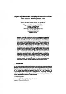
Figure 1: Five simulations of a simple Monte-Carlo tree search. Each simulation has an outcome of 1 for a black win or 0 for a white win (square). At each simulation a new node (star) is added into the search tree. The value of each node in the search tree (circles and star) is then updated to count the number of black wins, and the total number of visits (wins/visits).
5
limitations are still an issue, it is also possible to wait several simulations before adding a new node, or to prune old nodes as the search progresses. Figure 1 illustrates several steps of the MCTS algorithm. It is also possible to compute other statistics by Monte-Carlo tree search, for example the max outcome, which may evaluate positions more rapidly but is also sensitive to outliers [15], or an intermediate statistic between mean and max outcome [1]. However, the mean outcome has proven to be the most robust and effective statistic in Go and other domains. 2.5. UCT Greedy action selection can often be an inefficient way to construct a search tree, as it will typically avoid searching actions after one or more poor outcomes, even if there is significant uncertainty about the value of those actions. To explore the search tree more efficiently, the principle of optimism in the face of uncertainty can be applied, which favours the actions with the greatest potential value. To implement this principle, each action value receives a bonus that corresponds to the amount of uncertainty in the current value of that state and action. The UCT algorithm applies this principle to Monte-Carlo tree search, by treating each state of the search tree as a multi-armed bandit, in which each action corresponds to an arm of the bandit [10].4 The tree policy selects actions by using the UCB1 algorithm, which maximises an upper confidence bound on the value of actions [18]. Specifically, the action value is augmented by an exploration bonus that is highest for rarely visited state-action pairs, and the tree policy selects the action a∗ maximising the augmented value, s
Q⊕ (s, a) = Q(s, a) + c
log N (s) N (s, a)
a∗ = argmax Q⊕ (s, a)
(7) (8)
a
where c is a scalar exploration constant and log is the natural logarithm. Pseudocode for the UCT algorithm is given in Algorithm 1. UCT is proven to converge on the minimax action value function [10]. As the number of simulations N grows to infinity, the root values converge in probability to the minimax action values, ∀a ∈ A, plim Q(s0 , a) = Q∗ (s0 , a). Furthermore, the n→∞
bias of the root values, E[Q(s0 , a) − Q∗ (s0 , a)], is O(log(n)/n), and the probability of selecting a suboptimal action, P r(argmax Q(s0 , a) 6= argmax Q∗ (s0 , a)), converges a∈A
a∈A
to zero at a polynomial rate. The performance of UCT can often be significantly improved by incorporating domain knowledge into the default policy [19, 20]. The UCT algorithm, using a carefully 4 In fact, the search tree is not a true multi-armed bandit, as there is no real cost to exploration during planning. In addition the simulation policy continues to change as the search tree is updated, which means that the payoff is non-stationary.
6
Algorithm 1 Two Player UCT procedure S IM D EFAULT(board) while not board.GameOver() do a = D EFAULT P OLICY(board) board.P lay(a) end while return board.BlackW ins() end procedure
procedure U CT S EARCH(s0 ) while time available do S IMULATE(board, s0 ) end while board.SetP osition(s0 ) return S ELECT M OVE(board, s0 , 0) end procedure
procedure S ELECT M OVE(board, s, c) legal = board.Legal() if board.BlackT oP � lay() then q
procedure S IMULATE(board, s0 ) board.SetP osition(s0 ) [s0 , ..., sT ] = S IM T REE(board) z = S IM D EFAULT(board) BACKUP([s0 , ..., sT ], z) end procedure
a∗ = argmax
Q(s, a) + c
a∈legal
log N (s) N (s,a)
�
else q � � N (s) a∗ = argmin Q(s, a) − c log N (s,a) a∈legal
end if return a∗ end procedure
procedure S IM T REE(board) c = exploration constant t=0 while not board.GameOver() do st = board.GetP osition() if st ∈ / tree then N EW N ODE(st ) return [s0 , ..., st ] end if a = S ELECT M OVE(board, st , c) board.P lay(a) t=t+1 end while return [s0 , ..., st−1 ] end procedure
procedure BACKUP([s0 , ..., sT ], z) for t = 0 to T do N (st ) = N (st ) + 1 N (st , at ) ++ t ,at ) Q(st , at ) += z−Q(s N (st ,at ) end for end procedure procedure N EW N ODE(s) tree.Insert(s) N (s) = 0 for all a ∈ A do N (s, a) = 0 Q(s, a) = 0 end for end procedure
7
A
B
C
D
E
F
G
H
J
9 8
territory
e yes
r u les
A
B
C
D
E
F
G
H
A 88
A
A
J
99 E
8
E
7
77
7
6
66
6
5
55
A
F
3
33
3
1
B A
B
C
D
E
D
C
F
G
F
11 E
H
J
A
B
C
2 1
E D
E
F
G
H
G
G
4
22
H H
G
44
B
G
5
4
2
9
9
J
G
B
C
D
E
F
G
H
J
W W W W W W W W W
9
8 W* w W W W W W W W
8
H
7
w
w
w W w
w
w W W
7
H
6
b
w
w
w
b
b
w
w
w
6
5
b
b
b
b
b
B
b
b
b
5
4
b B* b
B
B
B
B
B
B
4
3
B* B* B* b
b
B
B
B
B
3
2
B B* B* b
B
B
B
B
B
2
1
B* B* b
b
B
B
B
B
B
1
A
D
E
F
G
H
J
H
H
G
H G
B
C
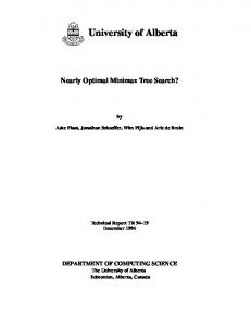
a) The White stones points Black toare play in atari and can be captured by playing at the Black to playmarked A. It is illegal for Black to play at B, as the stone would have no liberties. Black may, however, play at C to capture the stone at D. It is illegal for White to recapture immediately by playing at D, as this would repeat the position - it is a ko. b) The points marked E are eyes for Black. The black groups on the left can never be captured by White, they are alive. The points marked F are false eyes: the black stones on the right will eventually be captured by White and are dead. c) Groups of loosely connected white stones (G) and black stones (H). d) A final position. Dead stones (B∗, W ∗) are removed from the board. All surrounded intersections (B, W ) and all remaining stones (b, w) are counted for each player. If komi is 6.5 then Black wins by 8.5 points in this example.
Figure Black to play 2:
chosen default policy, has outperformed previous approaches to search in a variety of challenging games, including Go [19], General Game Playing [4], Amazons [5], Lines of Action [6], multi-player card games [7, 8], and real-time strategy games [9]. Much additional research in Monte-Carlo tree search has been developed in the context of computer Go, and is discussed in more detail in the next section. 3. Computer Go For many years, computer chess was considered to be “the drosophila of AI”,5 and a “grand challenge task” [21]. It provided a sandbox for new ideas, a straightforward performance comparison between algorithms, and measurable progress against human capabilities. With the dominance of alpha-beta search programs over human players now conclusive in chess [22], many researchers have sought out a new challenge. Computer Go has emerged as the “new drosophila of AI” [21], a “task par excellence” [23], and “a grand challenge task for our generation” [24]. Go has more than 10170 states and up to 361 legal moves. Its enormous search space is orders of magnitude too big for the alpha-beta search algorithms that have proven so successful in chess and checkers. Although the rules are simple, the emergent complexity of the game is profound. The long-term effect of a move may only be revealed after 50 or 100 additional moves. Professional Go players accumulate Go knowledge over a lifetime; mankind has accumulated Go knowledge over several millennia. For the last 30 years, attempts to encode this knowledge in machine usable form have led to a positional understanding that is at best comparable to weak amateur-level humans.
8
Beginner 30 kyu
Master 1 kyu 1 dan
Professional 7 dan 1 dan
9 dan
Figure 3: Performance ranks in Go, in increasing order of strength from left to right.
3.1. The Rules of Go The game of Go is usually played on a 19 × 19 grid, with 13 × 13 and 9 × 9 as popular alternatives. Black and White play alternately, placing a single stone on an intersection of the grid. Stones cannot be moved once played, but may be captured. Sets of adjacent, connected stones of one colour are known as blocks. The empty intersections adjacent to a block are called its liberties. If a block is reduced to zero liberties by the opponent, it is captured and removed from the board (Figure 2a, A). Stones with just one remaining liberty are said to be in atari. Playing a stone with zero liberties is illegal (Figure 2a, B), unless it also reduces an opponent block to zero liberties. In this case the opponent block is captured, and the player’s stone remains on the board (Figure 2a, C). Finally, repeating a previous board state is illegal.6 A situation in which a repeat could otherwise occur is known as ko (Figure 2a, D). A connected set of empty intersections that is wholly enclosed by stones of one colour is known as an eye. One natural consequence of the rules is that a block with two eyes can never be captured by the opponent (Figure 2b, E). Blocks which cannot be captured are described as alive; blocks which will certainly be captured are described as dead (Figure 2b, F ). A loosely connected set of stones is described as a group (Figure 2c, G, H). Determining the life and death status of a group is a fundamental aspect of Go strategy. The game ends when both players pass. Dead blocks are removed from the board (Figure 2d, B∗, W ∗). In Chinese rules, all alive stones, and all intersections that are enclosed by a player, are counted as a point of territory for that player (Figure 2d, B, W ).7 Black always plays first in Go; White receives compensation, known as komi, for playing second. The winner is the player with the greatest territory, after adding komi for White. 3.2. Go Ratings Human Go players are rated on a three-class scale, divided into kyu (beginner), dan (master), and professional dan ranks (see Figure 3). Kyu ranks are in descending order of strength, whereas dan and professional dan ranks are in ascending order. At amateur level, the difference in rank corresponds to the number of handicap stones required by the weaker player to ensure an even game.8 5 Drosophila
is the fruit fly, the most extensively studied organism in genetics research. exact definition of repeating differs subtly between different rule sets. 7 The Japanese scoring system is somewhat different, but usually has the same outcome. 8 The difference between 1 kyu and 1 dan is normally considered to be 1 stone. 6 The
9
The majority of computer Go programs compete on the Computer Go Server (CGOS). This server runs an ongoing rapid-play tournament of 5 minute games for 9 × 9 and 20 minute games for 19 × 19 boards. The Elo rating of each program on the server is continually updated. The Elo scale on CGOS assumes a logistic distribution with winning 1 probability P r(A beats B) = µB −µA , where µA and µB are the Elo ratings for 1+10
400
player A and player B respectively. On this scale, a difference of 200 Elo corresponds to a 75% winning rate for the stronger player, and a difference of 500 Elo corresponds to a 95% winning rate. Following convention, the open source Go program GnuGo (level 10) anchors this scale with a rating of 1800 Elo. 3.3. Handcrafted Heuristics In many other classic games, handcrafted heuristic functions have proven highly effective. Basic heuristics such as material count and mobility, which provide reasonable estimates of goodness in checkers, chess and Othello [25], are next to worthless in Go. Stronger heuristics have proven surprisingly hard to design, despite several decades of endeavour [26]. Until recently, most Go programs incorporated very large quantities of expert knowledge, in a pattern database containing many thousands of manually inputted patterns, and typically including expert knowledge such as fuseki (opening patterns), joseki (corner patterns), and tesuji (tactical patterns). Traditional Go programs use these databases to generate plausible moves that match one or more patterns. The pattern database accounts for a large part of the development effort in a traditional Go program, sometimes requiring many man-years of effort from expert Go players. The Many Faces of Go9 uses local alpha-beta searches to determine the life or death status of blocks and groups. A global alpha-beta search is used to evaluate full-board positions, using a heuristic function of the local search results. Pattern databases are used to generate moves in both the local and global searches. The program GnuGo10 uses pattern databases and specialised search routines to determine local subgoals such as capture, connection, and eye formation. The local status of each subgoal is used to estimate the overall benefit of each legal move. 3.4. Reinforcement Learning in Go Reinforcement learning can be used to train a value function that predicts the eventual outcome of the game from a given state. The learning program can be rewarded by the score at the end of the game, or by a reward of 1 if Black wins and 0 if White wins. Surprisingly, the less informative binary signal has proven more successful [1], as it encourages the agent to favour risky moves when behind, and calm moves when ahead. Expert Go players will frequently play to minimise the uncertainty in a position once they judge that they are ahead in score; this behaviour cannot be replicated by simply maximising the expected score. Despite this shortcoming, the final score has been widely used as a reward signal [27, 28, 29, 30]. 9 http://www.smart-games.com/manyfaces.html 10 http://www.gnu.org/software/gnugo
10
Schraudolph et al. [27] exploit the symmetries of the Go board in a convolutional neural network. The network predicts the final territory status of a particular target intersection. It receives one input from each intersection (−1, 0 or +1 for White, Empty and Black respectively) in a local region around the target, and outputs the predicted territory for the target intersection. The global position is evaluated by summing the territory predictions for all intersections on the board. Weights are shared between rotationally and reflectionally symmetric patterns of input features, and between all target intersections. They train their multilayer perceptron using T D(0), using a reward signal corresponding to the final territory value of the intersection. The network outperformed a commercial Go program, The Many Faces of Go, when set to a low playing level in 9 × 9 Go, after just 3,000 self-play training games. Dahl’s Honte [29] and Enzenberger’s NeuroGo III [30] use a similar approach to predicting the final territory. However, both programs learn intermediate features that are used to input additional knowledge into the territory evaluation network. Honte has one intermediate network to predict local moves and a second network to evaluate the life and death status of groups. NeuroGo III uses intermediate networks to evaluate connectivity and eyes. Both programs achieved single-digit kyu ranks; NeuroGo won the silver medal at the 2003 9 × 9 Computer Go Olympiad. RLGO 1.0 [31] uses a simpler but more computationally efficient approach to reinforcement learning. It uses a million local shape features to enumerate all possible 1 × 1, 2 × 2 and 3 × 3 configurations of Black, White and empty intersections, at every possible location on the board. The value of a state is estimated by a linear combination of the local shape features that are matched in that state. The weights of these features are trained offline by temporal-difference learning from games of self-play, and sharing weights between symmetric local shape features. The basic version of RLGO was rated at 1350 Elo on the 9 × 9 Computer Go Server. RLGO 2.4 [32, 13] applies the same reinforcement learning approach online. It applies temporal-difference learning to simulated games of self-play that start from the current state: a form of simulation-based search. At every move, the value function is re-trained in real-time, specialising on the tactics and strategies that are most relevant to the current position. This approach boosted RLGO’s rating to 2100 Elo on CGOS, outperforming traditional Go programs and resulting in the strongest 9 × 9 Go program not based on Monte-Carlo tree search. 3.5. Monte Carlo Simulation in Go In contrast to traditional search methods, Monte-Carlo simulation evaluates the current position dynamically, rather than storing knowledge about all positions in a static evaluation function. This makes it an appealing choice for Go, where, as we have seen, the number of possible positions is particularly large, and position evaluation is particularly challenging. The first Monte-Carlo Go program, Gobble [33], simulated many games of selfplay from the current state s. It combined Monte-Carlo evaluation with two novel ideas: the all-moves-as-first heuristic, and ordered simulation. The all-moves-as-first heuristic assumes that the value of a move is not significantly affected by changes elsewhere on the board. The value of playing action a immediately is estimated by the
11
average outcome of all simulations in which action a is played at any time. We formalise this idea more precisely in Section 4.1. Gobble also used ordered simulation to sort all moves according to their estimated value. This ordering is randomly perturbed according to an annealing schedule that cools down with additional simulations. Each simulation then plays out all moves in the prescribed order. Gobble itself played weakly, with an estimated rating of around 25 kyu. Bouzy and Helmstetter developed the first competitive Go programs based on MonteCarlo simulation [15]. Their basic framework simulates many games of self-play from the current state s, for each candidate action a, using a uniform random simulation policy; the value of a is estimated by the average outcome of these simulations. The only domain knowledge is to prohibit moves within eyes; this ensures that games terminate within a reasonable timeframe. Bouzy and Helmstetter also investigated a number of extensions to Monte-Carlo simulation, several of which are precursors to the more sophisticated algorithms used now: 1. Progressive pruning is a technique in which statistically inferior moves are removed from consideration [34]. 2. The all-moves-as-first heuristic, described above. 3. The temperature heuristic uses a softmax simulation policy to bias the random moves towards the strongest evaluations. The softmax policy selects actions Q(s,a)/τ with a probability π(s, a) = P e eQ(s,b)/τ , where τ is a constant temperature b∈legal
parameter controlling the overall level of randomness.11 4. The minimax enhancement constructs a full width search tree, and separately evaluates each node of the search tree by Monte-Carlo simulation. Selective search enhancements were also tried [35]. Bouzy also tracked statistics about the final territory status of each intersection after each simulation [36]. This information is used to influence the simulations towards disputed regions of the board, by avoiding playing on intersections which are consistently one player’s territory. Bouzy also incorporated pattern knowledge into the simulation player [20]. Using these enhancements his program Indigo won the bronze medal at the 2004 and 2006 19 × 19 Computer Go Olympiads. It is surprising that a Monte-Carlo technique, originally developed for stochastic games such as backgammon [16], Poker [14] and Scrabble [17] should succeed in Go. Why should an evaluation that is based on random play provide any useful information in the precise, deterministic game of Go? The answer, perhaps, is that Monte-Carlo methods successfully manage the uncertainty in the evaluation. A random simulation policy generates a broad distribution of simulated games, representing many possible futures and the uncertainty in what may happen next. As the search proceeds and more information is accrued, the simulation policy becomes more refined, and the distribution of simulated games narrows. In contrast, deterministic play represents perfect confidence in the future: there is only one possible continuation. If this confidence is 11 Gradually
reducing the temperature, as in simulated annealing, was not beneficial.
12
misplaced, then predictions based on deterministic play will be unreliable and misleading. Abramson [37] was the first to demonstrate that the expected value of a game’s outcome under random play is a powerful heuristic for position evaluation in deterministic games. 3.6. Monte-Carlo Tree Search in Go Monte-Carlo tree search was first introduced in the Go program Crazy Stone [1]. The Monte-Carlo value of each action is assumed to be normally distributed about the minimax value, Q(s, a) ∼ N (Q∗ (s, a), σ 2 (s, a)). During the first stage of simulation, the tree policy selects each action according to the estimated probability that its minimax value is better than the Monte-Carlo value of the best action a∗ , π(s, a) ≈ P r(Q∗ (s, a) > Q(s, a∗ )). During the second stage of simulation, the default policy selects moves with a probability proportional to a handcrafted urgency heuristic. Using these techniques, Crazy Stone exceeded 1800 Elo on CGOS, achieving equivalent performance to traditional Go programs such as GnuGo and The Many Faces of Go. Crazy Stone won the gold medal at the 2006 9 × 9 Computer Go Olympiad. The Go program MoGo introduced the UCT algorithm to computer Go [19, 38]. Instead of the Gaussian approximation used in Crazy Stone, MoGo treats each state in the search tree as a multi-armed bandit. There is one arm of the bandit for each legal move, and the payoff from an arm is the outcome of a simulation starting with that move. During the first stage of simulation, the tree policy selects actions using the UCB1 algorithm. During the second stage of simulation, MoGo uses a default policy based on specialised domain knowledge. Unlike the enormous pattern databases used in traditional Go programs, MoGo’s patterns are extremely simple. Rather than suggesting the best move in any situation, these patterns are intended to produce local sequences of plausible moves. They can be summarised by applying four prioritised rules after any opponent move a: 1. If a put some of our stones into atari, play a saving move at random. 2. Otherwise, if one of the 8 intersections surrounding a matches a simple pattern for cutting or hane, randomly play one. 3. Otherwise, if any opponent stone can be captured, play a capturing move at random. 4. Otherwise play a random move. The default policy used by MoGo is handcrafted. In contrast, a second version of Crazy Stone uses supervised learning to train the pattern weights for its default policy [2]. The relative strength of patterns is estimated by assigning an Elo rating to each pattern, much like a tournament between games players. In this approach, the pattern selected by a human player is considered to have won against all alternative patterns. Crazy Stone uses the minorisation-maximisation algorithm to estimate the Elo rating of simple 3 × 3 patterns and features. The default policy selected actions with a probability proportional to the matching pattern strengths. A more complicated set of 17,000 patterns, harvested from expert games, was used to progressively widen the search tree. Using the UCT algorithm, MoGo and Crazy Stone significantly outperformed all previous 9 × 9 Go programs, and beginning a new era in computer Go. 13
4. Rapid Action Value Estimation Monte-Carlo tree search separately estimates the value of each state and each action in the search tree. As a result, it cannot generalise between related positions or related moves. To determine the best move, many simulations must be performed from all states and for all actions. The RAVE algorithm uses the all-moves-as-first heuristic, from each node of the search tree, to estimate the value of each action. RAVE provides a simple way to share knowledge between related nodes in the search tree, resulting in a rapid, but biased estimate of the action values. This biased estimate can often determine the best move after just a handful of simulations, and can be used to significantly improve the performance of the search algorithm. 4.1. All-Moves-As-First In incremental games such as computer Go, the value of a move is often unaffected by moves played elsewhere on the board. The underlying idea of the all-moves-as-first (AMAF) heuristic [33] (see Section 3.5) is to have one general value for each move, ˜ π (s, a) to be the regardless of when it is played. We define the AMAF value function Q expected outcome z from state s, when following joint policy π for both players, given that action a was selected at some subsequent turn, ˜ π (s, a) = Eπ [z|st = s, ∃u ≥ t s.t. au = a] Q
(9)
The AMAF value function provides a biased estimate of the true action value func˜ a), depends on the particular state s and action a, tion. The level of bias, B(s, ˜ π (s, a) = Qπ (s, a) + B(s, ˜ a) Q
(10)
˜ π (s, a). The all-moves-asMonte-Carlo simulation can be used to approximate Q ˜ first value Q(s, a) is the mean outcome of all simulations in which action a is selected at any turn after s is encountered, ˜ a) = Q(s,
N (s) X 1 ˜Ii (s, a)zi , ˜ N (s, a) i=1
(11)
where ˜Ii (s, a) is an indicator function returning 1 if state s was encountered at any step t of the ith simulation, and action a was selected at any step u >= t, or 0 otherwise; ˜ (s, a) = PN (s) ˜Ii (s, a) counts the total number of simulations used to estimate and N i=1 the AMAF value. Note that Black moves and White moves are considered to be distinct actions, even if they are played at the same intersection. In order to select the best move with reasonable accuracy, Monte-Carlo simulation requires many simulations from every candidate move. The AMAF heuristic provides orders of magnitude more information: every move will typically have been tried on several occasions, after just a handful of simulations. If the value of a move really is unaffected, at least approximately, by moves played elsewhere, then this can result in a much faster rough estimate of the value.
14
a
τ(s) s a
b
a
b
a
a
Q(s, b) = 2/3 ˜ a) = 3/5 Q(s, ˜ b) = 2/5 Q(s,
b
0
0
Q(s, a) = 0/2
1
0
1
1
Figure 4: An example of using the RAVE algorithm to estimate the value of Black moves a and b from state s. Six simulations have been executed from state s, with outcomes shown in the bottom squares. Playing move a immediately led to two losses, and so Monte-Carlo estimation favours move b. However, playing move a at any subsequent time led to three wins out of five, and so the RAVE algorithm favours move a. Note that the simulation starting with move a from the root node does not belong to the subtree τ (s) and ˜ a). does not contribute to the AMAF estimate Q(s,
4.2. RAVE The RAVE algorithm combines Monte-Carlo tree search with the all-moves-as-first heuristic. Instead of computing the MC value (Equation 3) of each node of the searchtree, (s, a) ∈ T , the AMAF value (Equation 11) of each node is computed. Every state in the search tree, s ∈ T , is the root of a subtree τ (s) ⊆ S. If a simulation visits state st at step t, then all subsequent states visited in that simulation, su such that u ≥ t, are in the subtree of st , su ∈ τ (st ). This includes all states su ∈ /T visited by the default policy in the second stage of simulation. The basic idea of RAVE is to generalise over subtrees. The assumption is that the value of action a in state s will be similar from all states within subtree τ (s). Thus, the value of a is estimated from all simulations starting from s, regardless of exactly when a is played. When the AMAF values are used to select an action at in state st , the action with ˜ t , b). In princimaximum AMAF value in subtree τ (st ) is selected, at = argmax Q(s b
˜ k , ·), from ancestor subtrees, ple it is also possible to incorporate the AMAF values, Q(s τ (sk ) such that k < t. However, in our experiments, combining ancestor AMAF values did not appear to confer any advantage. RAVE is closely related to the history heuristic in alpha-beta search [39]. During
15
the depth-first traversal of the search tree, the history heuristic remembers the success12 of each move at various depths; the most successful moves are tried first in subsequent positions. RAVE is similar, but because it is a best-first not depth-first search, it must store values for each subtree. In addition, RAVE takes account of the success of moves made outside of the search tree by the default policy. 4.3. MC–RAVE The RAVE algorithm learns very quickly, but it is often wrong. The principal assumption of RAVE, that a particular move has the same value across an entire subtree, is frequently violated. There are many situations, for example during tactical battles, in which nearby changes can completely change the value of a move: sometimes rendering it redundant; sometimes making it even more vital. Even distant moves can significantly affect the value of a move, for example playing a ladder-breaker in one corner can radically alter the value of playing a ladder in the opposite corner. The MC–RAVE algorithm overcomes this issue, by combining the rapid learning of the RAVE algorithm with the accuracy and convergence guarantees of Monte-Carlo tree search. There is one node n(s) for each state s in the search tree. Each node contains a ˜ a), MC total count N (s), and for each a ∈ A, an MC value Q(s, a), AMAF value Q(s, ˜ count N (s, a), and AMAF count N (s, a). To estimate the overall value of action a in state s, we use a weighted sum Q? (s, a) ˜ a), of the MC value Q(s, a) and the AMAF value Q(s, ˜ a) Q? (s, a) = (1 − β(s, a))Q(s, a) + β(s, a)Q(s,
(12)
where β(s, a) is a weighting parameter for state s and action a. It is a function of the statistics for (s, a) stored in node n(s), and provides a schedule for combining the MC and AMAF values. When only a few simulations have been seen, we weight the AMAF value more highly, β(s, a) ≈ 1. When many simulations have been seen, we weight the Monte-Carlo value more highly, β(s, a) ≈ 0. As with Monte-Carlo tree search, each simulation is divided into two stages. During the first stage, for states within the search tree, st ∈ T , actions are selected greedily, so as to maximise the combined MC and AMAF value, a = argmax Q? (st , b). During b
the second stage of simulation, for states beyond the search tree, st ∈ / T , actions are selected by a default policy. After each simulation s0 , a0 , s1 , a1 , ..., sT with outcome z, both the MC and AMAF values are updated. For every state st in the simulation that is represented in the search tree, st ∈ T , the values and counts of the corresponding node n(st ) are updated, 12 A
successful move in alpha-beta either causes a cut-off, or has the best minimax value.
16
N (st ) ← N (st ) + 1
(13)
N (st , at ) ← N (st , at ) + 1
(14)
Q(st , at ) ← Q(st , at ) +
(15)
z − Q(st , at ) N (st , at )
In addition, the AMAF value is updated for every subtree. For every state st in the simulation that is represented in the tree, st ∈ T , and for every subsequent action of the simulation au with the same colour to play, i.e. u ≥ t and t = u mod 2, the AMAF value of (st , au ) is updated according to the simulation outcome z, ˜ (st , au ) ← N ˜ (st , au ) + 1 N
(16)
˜ ˜ t , au ) ← Q(s ˜ t , au ) + z − Q(st , au ) Q(s ˜ N (st , au )
(17)
If multiple moves are played at the same intersection during a simulation, then this update is only performed for the first move at the intersection. If an action au is legal in state su , but illegal in state st , then no update is performed for this move. 4.4. UCT–RAVE The UCT algorithm extends Monte-Carlo tree search to use the optimism-in-theface-of-uncertainty principle, by incorporating a bonus based on an upper confidence bound of the current value. Similarly, the MC–RAVE algorithm can also incorporate an exploration bonus, s log N (s) , (18) Q⊕ ? (s, a) = Q? (s, a) + c N (s, a) Actions are then selected during the first stage of simulation to maximise the aug13 mented value, a = argmax Q⊕ ? (s, b). We call this algorithm UCT–RAVE. b
If the schedule decreases to zero in all nodes, ∀s ∈ T , a ∈ A, lim β(s, a) = 0, N →∞
then the asymptotic behaviour of UCT–RAVE is equivalent to UCT. The asymptotic convergence properties of UCT (see Section 2) therefore also apply to UCT–RAVE. We now describe two different schedules which have this property. 4.5. Hand-Selected Schedule One hand-selected schedule for MC–RAVE uses an equivalence parameter k,
13 The original UCT-RAVE algorithm also included the RAVE count in the exploration term [11]. However, it is hard to justify explicit RAVE exploration: many actions will be evaluated by AMAF, regardless of which action is actually selected at turn t.
17
Winning rate against GnuGo 3.7.10
Combining Online and Offline Knowledge in UCT
state. We introduce a sim knowledge, which increase without biasing its asymp
0.7 UCT MC-RAVE
0.65 0.6
We modify UCT to incorp tion Qprior (s, a). When a is added to the UCT repre value according to our pri
0.55 0.5 0.45 0.4 0.35 0.3 0.25 0.2 1
10
100 k
1000
10000
n(s, a) ← QUCT (s, a) ←
The number nprior estima the prior val of episodes t different settings of the equivalence parameter k. The bars achieve an estimate of sim indicate the standard error. Each point of the plot is an isation, the value function sgames. average over 2300 complete mal UCT update (see eq k β(s, a) = (19)note the new UCT algori 3N (s) + k by U CT (π, Qprior ). where k specifies the number of simulations at which the Monte-Carlo value and the ! AMAF value should be given equal weight, β(s, a) = 21 , A similar modification can log m(s) ⊕ algorithm, by initialising t QRAV E (s, a) = QRAV E (s, a) + c s m(s, a) to prior knowledge, 1 k = ! (20) 2 3N (s)k+ k m(s, a) β(s, a) 1= k 3n(s) + k = (21) QRAV E (s, a) 4 3N (s) + k ⊕ ⊕ QUR (s, a) = β(s, k=N (s) a)QRAV E (s, a) (22) ⊕ We compare several me + (1 − β(s, a))Q (s, a) We tested MC–RAVE in the Go program MoGo,⊕usingUCT the hand-selected schedule (s) policy = argmax (s,for a)different settings of theknowledge in 9 × 9 Go. UR in Equation (19) and π the default describedQ inUR [19], a equivalence parameter k. For each setting, we played a 2300 game match againstheuristic, Qeven (s, a) = 0.5 " GnuGo 3.7.10 (level 10). The results are shown in Figure 5, and compared to Monte-tions encountered on-polic where m(s) = a m(s, a). The equivalence parameter Carlo tree search, using 3,000 simulations per move for both algorithms. The winningond, we use a grandfathe controlsvaried the number of and episodes of experience whenRAVE. rate usingkMC–RAVE between 50% 60%, compared to 24% without QUCT (st−2 , a), to indicate both estimates are given equal weight. Maximum performance is achieved with an equivalence parameter of 1,000 or more, P to play is usually similar indicating that the rapid action value estimate is more reliable than standard MonteWe tested the new algorithm U CT (πMoGofrom ), usCarlo simulation until several thousand simulations haveRAV beenEexecuted state s. with P to play. Third, we ing the default policy πMoGo , for different settings of QMoGo (s, a). This heuris the equivalence parameter k. For each setting, we greedy action selection wo played a 2300 game match against GnuGo 3.7.10 (level default policy πMoGo (s, a) 18 8). The results are shown in Figure 4, and compared to combination of binary fea the U CT (πMoGo ) algorithm with 3000 simulations per offline by T D(λ) (see sect move. The winning rate using U CTRAV E varies beFor each source of prior kn tween 50% and 60%, compared to 24% without rapid alent experience mprior (s, estimation. Maximum performance is achieved with stant values of Meq . We an equivalence parameter of 1000 or more. This inU CT (π ,Q )
Figure rate U CTRAV ) with Figure 5: Winning rate4. of Winning MC–RAVE with 3,000of simulations per move 3.7.103000 (level 10) incontained in E (πagainst M oGoGnuGo 9 × 9 Go, for different settings of the equivalence parameter k. The bars indicate the standard simulations per move against GnuGo 3.7.10 (level 8), error. for Eachthe number point of the plot is an average over 2300 complete games.
4.6. Minimum MSE Schedule The schedule presented in Equation 19 is somewhat heuristic in nature. We now develop a more principled schedule, which selects β(s, a) so as to minimise the mean squared error in the combined estimate Q? (s, a). 4.6.1. Assumptions To derive our schedule, we make a simplified statistical model of MC–RAVE. Our first assumption is that the policy π is held constant. Under this assumption, the outcome of each Monte-Carlo simulation, when playing action a from state s, is an independent and identically distributed (i.i.d.) Bernoulli random variable. Furthermore, the outcome of each AMAF simulation, when playing action a at any turn following state s, is also an i.i.d. Bernoulli random variable, P r(z = 1|st = s, at = a) = Qπ (s, a) P r(z = 0|st = s, at = a) = 1 − Qπ (s, a) ˜ π (s, a) P r(z = 1|st = s, ∃u ≥ t s.t. au = a) = Q ˜ π (s, a) P r(z = 0|st = s, ∃u ≥ t s.t. au = a) = 1 − Q
(23) (24) (25) (26)
It follows that the total number of wins, after N (s, a) simulations in which action a was played from state s, is binomially distributed. Similarly, the total number of wins, ˜ (s, a) simulations in which action a was played at any turn following state s, is after N binomially distributed, N (s, a)Q(s, a) ∼ Binomial(N (s, a), Qπ (s, a)) ˜ (s, a)Q(s, ˜ a) ∼ Binomial(N ˜ (s, a), Q ˜ π (s, a)) N
(27) (28)
Our second assumption is that these two distributions are independent, so that the MC and AMAF values are uncorrelated. In fact, the same simulations used to compute the MC value are also used to compute the AMAF value, which means that the values are certainly correlated. Furthermore, as the tree develops over time, the simulation policy changes. This means that outcomes are not i.i.d. and that the total number of wins is not in fact binomially distributed. Nevertheless, we believe that these simplifications do not significantly affect the performance of the schedule in practice. 4.6.2. Derivation To simplify our notation, we consider a single state s and action a. We denote the number of Monte-Carlo simulations by n = N (s, a) and the number of simulations ˜ (s, a), and abbreviate the schedule by used to compute the AMAF value by n ˜ = N β = β(s, a). We denote the estimated mean, bias (with respect to Qπ (s, a)) and variance of the MC, AMAF and combined values respectively by µ, µ ˜, µ? ; b, ˜b, b? and σ2 , σ ˜ 2 , σ?2 , and the mean squared error of the combined value by e2? ,
19
µ = Q(s, a) ˜ a) µ ˜ = Q(s,
(29) (30)
µ? = Q? (s, a)
(31)
π
π
b = Q (s, a) − Q (s, a) = 0 ˜b = Q ˜ π (s, a) − Qπ (s, a) = B(s, ˜ a)
b? =
Qπ? (s, a)
2
π
− Q (s, a) π
2
σ = E[(Q(s, a) − Q (s, a)) |N (s, a) = n] ˜ a) − Q ˜ π (s, a))2 |N ˜ (s, a) = n σ ˜ 2 = E[(Q(s, ˜] σ?2 e2?
˜ (s, a) = n = n, N ˜] ˜ (s, a) = n = E[(Q? (s, a) − Q (s, a)) |N (s, a) = n, N ˜] = E[(Q? (s, a) −
Qπ? (s, a))2 |N (s, a) π 2
(32) (33) (34) (35) (36) (37) (38)
We start by decomposing the mean squared error of the combined value into the bias and variance of the MC and AMAF values respectively, making use of our second assumption that these values are independently distributed, e2? = σ?2 + b2?
(39)
= (1 − β) σ + β σ ˜ + (β˜b + (1 − β)b)2 = (1 − β)2 σ 2 + β 2 σ ˜ 2 + β 2˜b2 2 2
2 2
(40) (41)
Differentiating with respect to β and setting to zero, 0 = 2β σ ˜ 2 − 2(1 − β)σ 2 + 2β˜b2
(42)
β=
(43)
2
σ2
σ +σ ˜ 2 + ˜b2
We now make use of our first assumption that the MC and AMAF values are binomially distributed, and estimate their variance, Qπ (s, a)(1 − Qπ (s, a)) µ? (1 − µ? ) ≈ N (s, a) n π π ˜ (s, a)) ˜ (s, a)(1 − Q Q µ? (1 − µ? ) σ ˜2 = ≈ ˜ n ˜ N (s, a)
σ2 =
β=
n ˜ ˜ n+n ˜ + n˜ nb2 /µ? (1 − µ? )
(44) (45) (46)
In roughly even positions, µ? ≈ 21 , we can further simplify the schedule, β=
n ˜ n+n ˜ + 4n˜ n˜b2 20
(47)
This equation still includes one unknown constant: the RAVE bias ˜b. This can either be evaluated empirically (by testing the performance of the algorithm with various constant values of ˜b), or by machine learning (by learning to predict the error between the AMAF value and the MC value, after many simulations). The former method is simple and effective; but the latter method could allow different biases to be identified for different types of position. 4.6.3. Results We compared the performance of MC–RAVE using the minimum MSE schedule, using the approximation in Equation 47, to the hand-selected schedule in Equation 19. For the minimum MSE schedule, we first identified the best constant RAVE bias in empirical tests. On a 9 × 9 board, the performance of MoGo using the minimum MSE schedule increased by 80 Elo (see Table 1). On a 19 × 19 board, the improvement was more than 100 Elo. 5. Heuristic Prior Knowledge We now introduce our second extension to Monte-Carlo tree search, heuristic MCTS. If a particular state s and action a is rarely encountered during simulation, then its Monte-Carlo value estimate is highly uncertain and very unreliable. Furthermore, because the search tree branches exponentially, the vast majority of nodes in the tree are only experienced rarely. The situation at the leaf nodes is worst of all: by definition each leaf node has been visited only once (otherwise a child node would have been added). In order to reduce the uncertainty for rarely encountered positions, we incorporate prior knowledge by using a heuristic evaluation function H(s, a) and a heuristic confidence function C(s, a). When a node is first added to the search tree, it is initialised according to the heuristic function, Q(s, a) = H(s, a) and N (s, a) = C(s, a). The confidence in the heuristic function is measured in terms of equivalent experience: the number of simulations that would be required in order to achieve a Monte-Carlo value of similar accuracy to the heuristic value.14 After initialisation, the value and count are updated as usual, using standard Monte-Carlo simulation. 5.1. Heuristic MC–RAVE The heuristic Monte-Carlo tree search algorithm can be combined with the MC– RAVE algorithm, described in pseudocode in Algorithm 2. When a new node n(s) is added to the tree, and for all actions a ∈ A, we initialise both the MC and AMAF values to the heuristic evaluation function, and initialise both counts to heuristic confidence functions C and C˜ respectively, 14 This
is equivalent to a beta prior when binary outcomes are used.
21
Algorithm 2 Heuristic MC–RAVE procedure M C –R AVE(s0 ) while time available do S IMULATE(board, s0 ) end while board.SetP osition(s0 ) return S ELECT M OVE(board, s0 , 0) end procedure
procedure S ELECT M OVE(board, s) legal = board.Legal() if board.BlackT oP lay() then return argmax E VAL(s, a) a∈legal
procedure S IMULATE(board, s0 ) board.SetP osition(s0 ) [s0 , a0 , ..., sT , aT ] = S IM T REE(board) [aT +1 , ..., aD ], z = S IM D EFAULT(board, T ) BACKUP([s0 , ..., sT ], [a0 , ..., aD ], z) end procedure procedure S IM D EFAULT(board, T ) t=T +1 while not board.GameOver() do at = D EFAULT P OLICY(board) board.P lay(at ) t=t+1 end while z = board.BlackW ins() return [aT +1 , ..., at−1 ], z end procedure procedure S IM T REE(board) t=0 while not board.GameOver() do st = board.GetP osition() if st ∈ / tree then N EW N ODE(st ) at = D EFAULT P OLICY(board) return [s0 , a0 , ..., st , at ] end if at = S ELECT M OVE(board, st ) board.P lay(at ) t=t+1 end while return [s0 , a0 , ..., st−1 , at−1 ] end procedure
22
else return argmin E VAL(s, a) a∈legal
end if end procedure procedure E VAL(s, a) b = pretuned constant bias value ˜ (s,a) N β = N (s,a)+N˜ (s,a)+4N ˜ (s,a)b2 (s,a)N ˜ a) return (1 − β)Q(s, a) + β Q(s, end procedure procedure BACKUP([s0 , ..., sT ], [a0 , ..., aD ], z) for t = 0 to T do N (st , at ) ++ t ,at ) Q(st , at ) += z−Q(s N (st ,at ) for u = t to D step 2 do if au ∈ / [at , at+2 , ..., au−2 ] then ˜ (st , au ) ++ N ˜ t ,at ) ˜ t , au ) += z−Q(s Q(s ˜ (st ,at ) N end if end for end for end procedure procedure N EW N ODE(board, s) tree.Insert(s) for all a ∈ board.Legal() do ˜ (s, a), Q(s, ˜ a) N (s, a), Q(s, a), N = H EURISTIC(board, a) end for end procedure
Q(s, a) ← H(s, a)
N (s, a) ← C(s, a) ˜ a) ← H(s, a) Q(s,
˜ (s, a) ← C(s, ˜ a) N X N (s) ← N (s, a)
(48) (49) (50) (51) (52)
a∈A
We compare four heuristic evaluation functions in 9 × 9 Go, using the heuristic MC–RAVE algorithm in the program MoGo. 1. The even-game heuristic, Qeven (s, a) = 0.5, makes the assumption that most positions encountered between strong players are likely to be close. 2. The grandfather heuristic, Qgrand (st , a) = Q(st−2 , a), sets the value of each node in the tree to the value of its grandfather. This assumes that the value of a Black move is usually similar to the value of that move, last time Black was to play. 3. The handcrafted heuristic, Qmogo (s, a), is based on the pattern-based rules that were successfully used in MoGo’s default policy. The heuristic was designed such that moves matching a “good” pattern were assigned a value of 1, moves matching a “bad” pattern were given value 0, and all other moves were assigned a value of 0.5. The good and bad patterns were identical to those used in MoGo, such that selecting moves greedily according to the heuristic, and breaking ties randomly, would exactly produce the default policy πmogo . 4. The local shape heuristic, Qrlgo (s, a), is computed from the linear combination of local shape features used in RLGO 1.0 (see Section 3.4). This heuristic is learnt offline by temporal difference learning from games of self-play. ˜ a) = For each heuristic evaluation function, we assign a heuristic confidence C(s, M , for various constant values of equivalent experience M . We played 2300 games between MoGo and GnuGo 3.7.10 (level 10). The MC–RAVE algorithm executed 3,000 simulations per move (see Figure 6). The value function learnt from local shape features, Qrlgo , outperformed all the other heuristics and increased the winning rate of MoGo from 60% to 69%. Maximum performance was achieved using an equivalent experience of M = 50, which indicates that Qrlgo is worth about as much as 50 simulations using all-moves-as-first. It seems likely that these results could be further improved by varying the heuristic confidence according to the particular position, based on the variance of the heuristic evaluation function. 5.2. Exploration and Exploitation The performance of Monte-Carlo tree search is greatly improved by carefully balancing exploration with exploitation. The UCT algorithm significantly outperforms a greedy tree policy in computer Go [19]. Surprisingly, this result does not appear 23
Combining Online and Offline Knowledge in UCT 0.75 Local Shape Features Handcrafted Heuristic Grandfather Heuristic Even Game Heuristic No Heuristic
Winning rate against GnuGo 3.7.10 default level
0.7
0.65
0.6
0.55
0.5
0.45
0.4
0
50
100
150
200
M Figure 5. Winning of U CT ) with 3000 MC–RAVE simulations per move against GnuGoper3.7.10 RAV E (πM oGo Figurerate 6: Winning rate of MoGo, using the heuristic algorithm, with 3,000 simulations move (level 8), using different prior knowledge as 3.7.10 initialisation. the standard error. function Each point of the against GnuGo (level 10) inThe 9 ×bars 9 Go.indicate Four different forms of heuristic were used (seeplot text).is an average over 2300 complete The games. bars indicate the standard error. Each point of the plot is an average over 2300 complete games.
Schraudolph, N., Dayan, P., & Sejnowski, T. (1994). ences. International Computer Chess Association Temporal difference learning of position evaluation Journal, 21, 84–99. to extend to the heuristic UCT–RAVE algorithm: the optimal exploration rate in our in the game of Go. Advances in Neural Information experiments was zero, i.e. greedy MC–RAVE with no exploration in the tree policy. Bruegmann, B. (1993). Monte-Carlo Go. Processing Systems 6 (pp. 817–824). San Francisco: We believe that the explanation lies in the nature of the RAVE algorithm. Even if Morgan Kaufmann. Buro, M. (1999). From simple sophisticated an action a is notfeatures selectedto immediately from position s, it will often be played at some evaluation functions. 1stthe International Silver,the D.,need Sutton, & M¨ uexploration, ller, M. (2007). Reinforcelater point in simulation. Conference This greatly reduces for R., explicit on Computers and Games (pp. ment learning of local shape in the game of Go. 20th because the values for126–145). all actions are continually updated, regardless of the initial move International Joint Conference on Artificial Intelliselection. Coulom, R. (2006). Efficient selectivity and backup op(pp. tens 1053–1058). However, we were only able to run thoroughgence tests with of thousands of simuerators in monte-carlo tree search. 5th International lations per move. It is possible that exploration again becomes MC– by the method Sutton, R. (1988).important Learningwhen to predict Conference on Computer and Games, 2006-05-29. RAVE is scaled up to millions of simulations per move. At this point a substantial of temporal differences. Machine Learning, 3, 9–44. Turin, Italy. number of nodes will be dominated by MC values rather than RAVE values, so that exploration at these nodes should beneficial.Sutton, R. (1990). Integrated architectures for learnEnzenberger, M. (2003). Evaluation in Go by abeneural ing, planning, and reacting based on approximating network using soft segmentation. 10th Advances in dynamic programming. 7th International ConferComputer Games Conference 5.3. Soft Pruning (pp. 97–108). ence on Machine Learning (pp. 216–224). Computer Go has a large branching factor and several pruning techniques, such Gelly, S., Wang, Y., Munos, R., & Teytaud, O. (2006). Sutton, R. (1996). in reinforcement as selective search and progressive widening (see Section 3), haveGeneralization been developed Modification of UCT with patterns in Monte-Carlo learning: Successful examplescan using sparse coarse to reduce the size of the search space [40]. Heuristic MCTS and MC–RAVE be Go (Technical Report 6062). INRIA. coding. in Neural Processing viewed as soft pruning techniques that focus on the highestAdvances valued regions of theInformation search Systems (pp. 1038–1044). Kocsis, L., &space Szepesvari, (2006). cutting Bandit off based without C. permanently any branches of the8search tree. Monte-Carlo planning. 15th European Conference on Machine Learning (pp. 282–293).
Sutton, R., & Barto, A. (1998). Reinforcement learning: An introduction. Cambridge, MA: MIT Press.
24 Wang, Y., & Gelly, S. (2007). Modifications of Schaeffer, J., Hlynka, M., & Jussila, V. (2001). Tempouct and sequence-like simulations for monte-carlo ral difference learning applied to a high-performance go. IEEE Symposium on Computational Intelligence game-playing program. 17th International Joint and Games, Honolulu, Hawaii (pp. 175–182). Conference on Artificial Intelligence (pp. 529–534).
Schedule Hand-selected Hand-selected Hand-selected Minimum MSE
Computation 3,000 sims per move 10,000 sims per move 10 minutes per game 10 minutes per game
Wins vs. GnuGo 69% 82% 92% 97%
CGOS rating 1960 2110 2320 2480∗
Table 1: Winning rate of MoGo against GnuGo 3.7.10 (level 10) when the number of simulations per move is increased. MoGo competed on CGOS, using heuristic MC–RAVE and the hand-selected schedule, in February 2007. The versions using 10 minutes per game modify the simulations per move according to the available time, from 300, 000 games in the opening to 20, 000 in the endgame. The asterisked version competed on CGOS in April 2007 using the minimum MSE schedule and additional parameter tuning.
A heuristic function provides a principled way to use prior knowledge to reduce the effective branching factor. Moves favoured by the heuristic function will be initialised with a high value, and tried much more often than moves with a low heuristic value. However, if the heuristic evaluation function is incorrect, then the initial value will drop off at a rate determined by the heuristic confidence function, and other moves will then be explored. The MC–RAVE algorithm also significantly reduces the effective branching factor. RAVE forms a fast, rough estimate of the value of each move. Moves with high RAVE values will quickly become favoured over moves with low RAVE values, which are soft pruned from the search tree. However, the RAVE values are only used initially, so that MC–RAVE never cuts branches permanently from the search tree. Heuristic MC–RAVE can often be wrong. The heuristic evaluation function can be inaccurate, and/or the RAVE estimate can be misleading. In this case, heuristic MC– RAVE will prioritise the wrong moves, and the best moves can be soft pruned and not tried again for many simulations. There are no guarantees that these algorithms will help performance. However, in practice they help more than they hurt, and on average over many positions, they provide a very significant performance advantage. 5.4. Performance of heuristic MC–RAVE in MoGo Our two extensions to MCTS, heuristic MCTS and MC–RAVE, increased the winning rate of MoGo against GnuGo, from 24% for UCT, up to 69% using heuristic MC–RAVE. However, these results were based on executing just 3,000 simulations per move, using the hand-selected schedule in Equation 19. When the number of simulations was increased, the overall performance of MoGo improved correspondingly. Table 1 shows how the performance of heuristic MC–RAVE scales with additional computation. The 2007 release version of MoGo used the heuristic MC–RAVE algorithm, the minimum MSE schedule in Equation 47, and an improved, handcrafted heuristic function.15 The scalability of the release version is shown in Figure 7, based on the results of a combined study over many thousands of computer hours [41]. This version of 15 Local
shape features were not used in the release version.
25
9x9 Scalability Study 3200 MoGo GnuGo 3.7.11
3000 2800 2600 2400
Elo rating
2200 2000 1800 1600 1400 1200 1000 800 600
26
27
28
29
210
211
212
213 214 215 216 217 Simulations per move
218
219
220
221
222
223
218
219
220
221
222
223
13x13 Scalability Study 3200 MoGo GnuGo 3.7.11
3000 2800 2600 2400
Elo rating
2200 2000 1800 1600 1400 1200 1000 800 600
26
27
28
29
210
211
212
213 214 215 216 217 Simulations per move
Figure 7: Scalability of MoGo (2007 release version), using data collected by members of the Computer Go mailing list [41]. Elo ratings were computed from a large tournament, consisting of several thousand games for each version of MoGo, using successive doublings of the number of simulations per move. Error bars indicate 95% confidence intervals in the Elo rating.
26
MoGo became the first program to achieve dan level at 9 × 9 Go; the first program to beat a professional human player at 9 × 9 Go; the highest rated program on the Computer Go Server for both 9 × 9 and 19 × 19 Go; the gold medal winner at the 2007 19 × 19 Computer Go Olympiad; and achieved a rating of 2 kyu at 19 × 19 Go against human players on the Kiseido Go Server. 6. Survey of Subsequent Work The results in the previous section were achieved by MoGo in 2007. We briefly survey subsequent work on heuristic MC–RAVE in a variety of other strong Go programs. The heuristic function of MoGo was substantially enhanced by initialising H(s, a), ˜ a) to hand-tuned values based on handcrafted rules and patterns [42]. C(s, a), and C(s, Supervised learning was also used to bias move selection towards patterns favoured in expert games. In addition, the handcrafted default policy was modified to increase the diversity of simulations, by playing in empty regions of the board; and to fix a known issue with life-and-death, by playing in the key point of simple dead shapes known as nakade. Using 100,000 simulations, the improved version of MoGo achieved a winning rate of 55% on 9 × 9 boards, and 53% on 19 × 19 boards, against the 2007 release version of MoGo. MoGo was also modified by massively parallelising the MC–RAVE algorithm to run on a cluster [43]. In order to avoid huge communication overheads, memory was only shared between the shallowest nodes in the search tree. The massively parallel version of MoGo Titan was run on 800 processors of Huygens, the Dutch national supercomputer. MoGo Titan defeated a 9 dan professional player, Jun-Xun Zhou, in 19 × 19 Go with 7 stones handicap. The program Zen has successfully combined MC–RAVE with more sophisticated domain knowledge. Zen became the first program to sustain a dan rank, on full-size 19 × 19 boards, against human players on the Kiseido Go Server (KGS). It is currently ranked at 4 dan, placing it within the top 5% of the 30,000 ranked human players on KGS. Several of the strongest traditional Go programs now combine their existing tactical and pattern knowledge with the heuristic MC–RAVE framework, including The Many Faces of Go, currently ranked at 2 dan on KGS and Aya, currently ranked at 1 dan. The open source program Fuego [44] extends the MC–RAVE algorithm to use additional rapid value estimates, using a variant of the minimum MSE schedule (see Equation 46). A parallelised version of Fuego defeated a 9 dan professional player in an even 9 × 9 game, and defeated a 6 dan amateur player with 4 stones handicap on a full size board.16 The latest versions of MoGo, Crazy Stone and the The Many Faces of Go have also achieved impressive victories against professional players on full size boards. Most recently, the program Erica combined heuristic MC–RAVE with a new technique, known as simulation balancing [45], to automatically tune the parameters of its 16 See
Human-Computer Go Challenges, http://www.computer-go.info/h-c/index.html.
27
Year 2006 2006 2006 2006 2007 2007 2007 2009 2010 2010
Program Indigo GnuGo Many Faces NeuroGo RLGO MoGo Crazy Stone Fuego Many Faces Zen
Description Pattern database, Monte-Carlo simulation Pattern database, alpha-beta search Temporal-difference learning, neural network Temporal-difference search
Variants of heuristic MC–RAVE
Elo 1400 1800 1800 1850 2100 2500 2500 2700 2700 2700
Table 2: Approximate Elo ratings, on the Computer Go Server, of 9 × 9 Go programs discussed in the text.
default policy [46]. Previous machine learning approaches have focused on optimising the strength of the default policy, under the assumption that a stronger policy will perform better in a Monte-Carlo search [1]. Unfortunately, in practice this assumption is often incorrect [11], and in general it can be difficult to find a default policy that performs well in Monte-Carlo search. The key idea of simulation balancing is to minimise the error between the Monte-Carlo value Q(s, a), and an oracle value computed by deep search. Erica used simulation balancing to train 2000 parameters of its default policy for 9 × 9 Go. Erica also won the gold medal in the 2010 19 × 19 Computer Go Olympiad, and is currently ranked at 3 dan on KGS. We provide a summary of the current state of the art in computer Go, based on ratings from the Computer Go Server (see Table 2) and the Kiseido Go Server (see Figure 8). Several of the programs described in Section 3 are included for comparison. 7. Conclusions For the last 30 years, computer Go programs have evaluated positions by using handcrafted heuristics that are based on human expert knowledge of shapes, patterns and rules. However, professional Go players often play moves according to intuitive feelings that are hard to express or quantify. Precisely encoding their knowledge into machine-understandable rules has proven to be a dead-end: a classic example of the knowledge acquisition bottleneck. Furthermore, traditional search algorithms, which are based on these handcrafted heuristics, cannot cope with the enormous state space and branching factor in the game of Go, and are unable to make effective use of additional computation time. This approach has led to Go programs that are at best comparable to weak amateur-level humans [26, 47]. In contrast, Monte-Carlo tree search requires no human knowledge in order to understand a position. Instead, positions are evaluated from the outcome of thousands of simulated games of self-play from that position. These simulated games are progressively refined to prioritise the selection of positions with promising evaluations. Over the course of many simulations, attention is focused selectively on narrow regions of the search space that are correlated with successful outcomes. Unlike traditional search
28
5 dan 4 dan
Zen
3 dan
ZenErica
2 dan
Zen
1 dan
Aya ManyFaces
Zen
1 kyu
Aya ManyFaces
CrazyStone
2 kyu
Fuego ManyFaces Aya
CrazyStoneMoGo
3 kyu
Aya
MoGo
ManyFaces
4 kyu
ManyFaces
ManyFaces
5 kyu
GnuGo*
6 kyu
GnuGo*
7 kyu 8 kyu Indigo MoGoAya* ManyFaces* 9 kyu
Aya*
10 kyu
Jul 06
Jan 07
Jul 07
Jan 08
Jul 08
Jan 09
Jul 09
Jan 10
Jul 10
Jan 11
Figure 8: Ranks of various Go programs discussed in the text on the Kiseido Go Server (KGS). Each Foo point represents the first date at which a program held the given rank for 20 consecutive games on KGS. Note that each program plays with different time controls, which may cause variations in rank; and that some programs play more regularly than others, which may cause variations in date. See http://senseis.xmp.net/?KGSBotRatings. *Version of GnuGo, Aya, Many Faces of Go based on traditional search with no Monte-Carlo.
algorithms, this approach scales well both with the size of the state space and branching factor, and also scale well with additional computation time. In practice, the strongest programs do make extensive use of expert human knowledge: both to improve the default policy and to define the prior knowledge. This knowledge accelerates the progress of the search, but does not affect its asymptotic optimality. On the Computer Go Server, using 9 × 9, 13 × 13 and 19 × 19 board sizes, traditional search programs are rated at around 1800 Elo, whereas Monte-Carlo programs, enhanced by RAVE and heuristic knowledge, are rated at over 2500 Elo using standard hardware17 (see Table 2). On1 the Kiseido Go Server, on full-size boards against human opposition, traditional search programs have reached 5 kyu, whereas the best MonteCarlo programs are rated at 4 dan (see Figure 8). The top programs are now competitive with top human professionals at 9 × 9 Go, and are winning handicap games against top human professionals at 19 × 19 Go. In the Go program Mogo, every doubling in computation power led to an increase 17 A
difference of 700 Elo corresponds to a 99% winning rate.
29
in playing strength of approximately 100 Elo points in 13 × 13 Go (see Figure 7) and perhaps even more in 19 × 19 Go. The strongest programs still lag far behind the strongest humans, but they are improving rapidly. Figure 8 shows that, after the initial jump in performance achieved by the first Monte-Carlo programs, computer Go programs have continued to improve by more than one rank every year. This new framework for Monte-Carlo tree search also extends beyond Go. Variants of heuristic MC–RAVE have outperformed previous search algorithms in other challenging games, such as Hex [48] and Havannah [49]. The challenging properties of Go are also characteristic of many of the hardest search, planning and decision-making problems. Immediate actions often have delayed, long-term consequences, leading to surprising complexity and enormous search spaces that are intractable to traditional search algorithms. Variants of heuristic MCTS and MC–RAVE are now outperforming previous approaches in challenging search spaces such as feature selection [50], POMDP planning [51], and natural language phrase generation [52]. Understanding how to achieve high performance in Go is opening up new possibilities for high performance AI in a wide variety of challenging problems. References [1] R. Coulom, Efficient selectivity and backup operators in Monte-Carlo tree search, in: 5th International Conference on Computer and Games, pp. 72–83. [2] R. Coulom, Computing Elo ratings of move patterns in the game of Go, International Computer Games Association Journal 30 (2007) 198–208. [3] S. Gelly, D. Silver, Achieving master level play in 9 x 9 computer Go, in: 23rd Conference on Artificial Intelligence, pp. 1537–1540. [4] H. Finnsson, Y. Bj¨ornsson, Simulation-based approach to general game playing, in: 23rd Conference on Artificial Intelligence, pp. 259–264. [5] R. Lorentz, Amazons discover Monte-Carlo, in: 6th International Conference on Computers and Games, pp. 13–24. [6] M. Winands, Y. Y. Bj¨ornsson, Evaluation function based Monte-Carlo LOA, in: 12th Advances in Computer Games Conference, pp. 33–44. [7] J. Sch¨afer, The UCT algorithm applied to games with imperfect information, Diploma Thesis. Otto-von-Guericke-Universit¨at Magdeburg, 2008. [8] N. Sturtevant, An analysis of UCT in multi-player games, in: 6th International Conference on Computers and Games, pp. 37–49. [9] R. Balla, A. Fern, UCT for tactical assault planning in real-time strategy games, in: 21st International Joint Conference on Artificial Intelligence, pp. 40–45. [10] L. Kocsis, C. Szepesvari, Bandit based Monte-Carlo planning, in: 15th European Conference on Machine Learning, pp. 282–293.
30
[11] S. Gelly, D. Silver, Combining online and offline learning in UCT, in: 17th International Conference on Machine Learning, pp. 273–280. [12] S. Gelly, A Contribution to Reinforcement Learning; Application to Computer Go, Ph.D. thesis, University of South Paris, 2007. [13] D. Silver, Reinforcement Learning and Simulation-Based Search in the Game of Go, Ph.D. thesis, University of Alberta, 2009. [14] D. Billings, L. P. Castillo, J. Schaeffer, D. Szafron, Using probabilistic knowledge and simulation to play poker, in: 16th National Conference on Artificial Intelligence, pp. 697–703. [15] B. Bouzy, B. Helmstetter, Monte-Carlo Go developments, in: 10th Advances in Computer Games Conference, pp. 159–174. [16] G. Tesauro, G. Galperin, On-line policy improvement using Monte-Carlo search, in: Advances in Neural Information Processing 9, pp. 1068–1074. [17] B. Sheppard, World-championship-caliber Scrabble, Artificial Intelligence 134 (2002) 241–275. [18] P. Auer, N. Cesa-Bianchi, P. Fischer, Finite-time analysis of the multi-armed bandit problem, Machine Learning 47 (2002) 235–256. [19] S. Gelly, Y. Wang, R. Munos, O. Teytaud, Modification of UCT with Patterns in Monte-Carlo Go, Technical Report 6062, INRIA, 2006. [20] B. Bouzy, Associating domain-dependent knowledge and Monte Carlo approaches within a Go program, Information Sciences, Heuristic Search and Computer Game Playing IV 175 (2005) 247–257. [21] J. McCarthy, AI as sport, Science 276 (1997) 1518–1519. [22] D. McClain, Once again, machine beats human champion at chess, New York Times, December 5th (2006). [23] A. Harmon, Queen, captured by mouse; more chess players use computers for edge, New York Times, February 6th (2003). [24] D. Mechner, All Systems Go, The Sciences 38 (1998). [25] J. Schaeffer, The games computers (and people) play, Advances in Computers 50 (2000) 189–266. [26] M. M¨uller, Computer Go, Artificial Intelligence 134 (2002) 145–179. [27] N. Schraudolph, P. Dayan, T. Sejnowski, Temporal difference learning of position evaluation in the game of Go, in: Advances in Neural Information Processing 6, pp. 817–824.
31
[28] M. Enzenberger, The integration of a priori knowledge into a Go playing neural network, http://www.cs.ualberta.ca/ emarkus/neurogo/neurogo1996.html, 1996. [29] F. Dahl, Honte, a Go-playing program using neural nets, in: Machines that learn to play games, Nova Science, 1999, pp. 205–223. [30] M. Enzenberger, Evaluation in Go by a neural network using soft segmentation, in: 10th Advances in Computer Games Conference, pp. 97–108. [31] D. Silver, R. Sutton, M. M¨uller, Reinforcement learning of local shape in the game of Go, in: 20th International Joint Conference on Artificial Intelligence, pp. 1053–1058. [32] D. Silver, R. Sutton, M. M¨uller, Sample-based learning and search with permanent and transient memories, in: 25th International Conference on Machine Learning, pp. 968–975. [33] B. Bruegmann, Monte-Carlo Go, http://www.cgl.ucsf.edu/go/Programs/Gobble.html, 1993. [34] B. Bouzy, Move pruning techniques for Monte-Carlo Go, in: 11th Advances in Computer Games Conference, pp. 104–119. [35] B. Bouzy, Associating shallow and selective global tree search with Monte Carlo for 9x9 Go, in: 4th International Conference on Computers and Games, pp. 67– 80. [36] B. Bouzy, History and territory heuristics for Monte-Carlo Go, New Mathematics and Natural Computation 2 (2006) 1–8. [37] B. Abramson, Expected-outcome: A general model of static evaluation, IEEE Transactions on Pattern Analysis and Machine Intelligence 12 (1990) 182–193. [38] Y. Wang, S. Gelly, Modifications of UCT and sequence-like simulations for Monte-Carlo Go, in: IEEE Symposium on Computational Intelligence and Games, Honolulu, Hawaii, pp. 175–182. [39] J. Schaeffer, The history heuristic and alpha–beta search enhancements in practice, IEEE Transactions on Pattern Analysis and Machine Intelligence PAMI-11 (1989) 1203–1212. [40] G. Chaslot, M. Winands, J. Uiterwijk, H. van den Herik, B. Bouzy, Progressive strategies for Monte-Carlo tree search, New Mathematics and Natural Computation 4 (2008) 343–357. [41] D. Dailey, 9x9 scalability study, http://cgos.boardspace.net/study/index.html, 2008. [42] G. Chaslot, L. Chatriot, C. Fiter, S. Gelly, J. Hoock, J. Perez, A. Rimmel, O. Teytaud, Combining expert, online, transient and online knowledge in Monte-Carlo exploration, in: 8th European Workshop on Reinforcement Learning. 32
[43] S. Gelly, J. Hoock, A. Rimmel, O. Teytaud, Y. Kalemkarian, The parallelization of Monte-Carlo planning, in: 6th International Conference in Control, Automation and Robotics, pp. 244–249. [44] M. M¨uller, M. Enzenberger, Fuego – An Open-source Framework for Board Games and Go Engine Based on Monte-Carlo Tree Search, Technical Report TR09-08, University of Alberta, Dept. of Computing Science, 2009. [45] D. Silver, G. Tesauro, Monte-Carlo simulation balancing, in: 26th International Conference on Machine Learning, pp. 119–126. [46] S. Huang, R. Coulom, S. Lin, Monte-Carlo simulation balancing in practice, in: 7th International Conference on Computers and Games, pp. 119–126. [47] B. Bouzy, T. Cazenave, Computer Go: an AI-oriented survey, Artificial Intelligence 132 (2001) 39–103. [48] B. Arneson, R. Hayward, P. Henderson, MoHex wins Hex tournament, International Computer Games Association Journal 32 (2009) 114–116. [49] F. Teytaud, O.Teytaud, Creating an Upper Confidence Tree program for Havannah, in: 12th Advances in Computer Games Conference, pp. 65–74. [50] R. Gaudel, M. Sebag, Feature selection as a one-player game, in: 27th International Conference on Machine Learning, pp. 359–366. [51] D. Silver, J. Veness, Online Monte-Carlo planning in large POMDPs, in: Advances in Neural Information Processing Systems 24. [52] J. Chevelu, T. Lavergne, Y. Lepage, T. Moudenc, Introduction of a new paraphrase generation tool based on Monte-Carlo sampling, in: 47th Annual Meeting of the Association for Computational Linguistics, pp. 249–252.
33