Jan 12, 2009 - 2 Autonomy in Communication-Challenged Environments. 11 ...... This requires fully integrated sensing, modeling and control, a much higher. 11 .... are controlled using high-level 'behavior algebra' in one, .... overlap and increase coverage. .... The core of the nested autonomy paradigm is the autonomous, ...
MOOS-IvP Nested Autonomy Prototype for Distributed Undersea Sensing User’s Guide H. Schmidt, M.R. Benjamin, A. Balasuriya, D. Battle, T. Schneider, and K. Cockrell Laboratory for Autonomous Marine Sensing Department Mechanical Engineering Massachusetts Institute of Technology, Cambridge MA
January 12, 2009
Abstract This paper provides an introductory description and User’s Guide for the MIT MOOS-IvP Undersea Autonomous Network Architecture, based on the Nested Autonomy paradigm, as implemented and operated on the fleet of Bluefin21 autonomous Underwater vehicles applied by the Laboratry for Autonomous Marine sensing for research and development into distributed acoustic sensing in the ocean.
2
Contents I
Introduction
10
1 Overview 10 1.1 Purpose and Scope of this Document . . . . . . . . . . . . . . . . . . . . . . . . . . . 10 1.2 Distributed Undersea Sensing and Observation . . . . . . . . . . . . . . . . . . . . . 10
II
Nested Autonomy Paradigm for Distributed Undersea Sensing
11
2 Autonomy in Communication-Challenged Environments
11
3 Nested Autonomy for Ocean Observation Systems
14
4 Concept of Operations 16 4.1 Field-level CONOPS . . . . . . . . . . . . . . . . . . . . . . . . . . . . . . . . . . . . 16 4.2 Cluster-level CONOPS . . . . . . . . . . . . . . . . . . . . . . . . . . . . . . . . . . . 17 4.3 Node-level CONOPS . . . . . . . . . . . . . . . . . . . . . . . . . . . . . . . . . . . . 18 5 Cluster Autonomy System
20
6 Platform Autonomy System 6.1 The MOOS-IvP Autonomy Architecture . 6.2 The Back-Seat Driver Paradigm . . . . . 6.3 Communication Connectivity . . . . . . 6.4 Autonomy States and State-Transitions 6.5 On-board, Real-time Signal Processing . 6.6 MOOS-IvP Simulation Environment . . .
21 21 21 22 24 26 27
III
. . . . . .
. . . . . .
. . . . . .
. . . . . .
. . . . . .
. . . . . .
. . . . . .
. . . . . .
. . . . . .
. . . . . .
. . . . . .
. . . . . .
. . . . . .
. . . . . .
. . . . . .
. . . . . .
. . . . . .
. . . . . .
. . . . . .
. . . . . .
. . . . . .
. . . . . .
. . . . . .
. . . . . .
. . . . . .
MIT-LAMS Nested Autonomy Prototype
28
7 MOOS-IvP Nested Autonomy Architecture 28 7.1 Sonar AUV MOOS Community . . . . . . . . . . . . . . . . . . . . . . . . . . . . . . 28
IV
IvP-Helm Autonomy for Undersea Sensing
32
8 Mission Planning and Control
32
9 Hierarchial State Representation 9.1 MOOS-IvP State Definitions . . 9.2 Mission Terminating States . . . 9.3 Deploy States . . . . . . . . . . . 9.3.1 Loiter Sub-States . . . . .
32 32 34 35 36
. . . .
. . . .
. . . .
. . . .
3
. . . .
. . . .
. . . .
. . . .
. . . .
. . . .
. . . .
. . . .
. . . .
. . . .
. . . .
. . . .
. . . .
. . . .
. . . .
. . . .
. . . .
. . . .
. . . .
. . . .
. . . .
. . . .
. . . .
. . . .
. . . .
9.4
9.3.2 Racetrack Sub-State . . 9.3.3 ZigZag Sub-state . . . . 9.3.4 Trail Sub-state . . . . . Prosecute States . . . . . . . . 9.4.1 Search Sub-State . . . . 9.4.2 Ambiguous Sub-State . 9.4.3 Tracking Sub-State . . . 9.4.4 Classification Sub-State
. . . . . . . .
. . . . . . . .
. . . . . . . .
. . . . . . . .
. . . . . . . .
. . . . . . . .
. . . . . . . .
. . . . . . . .
. . . . . . . .
. . . . . . . .
. . . . . . . .
. . . . . . . .
. . . . . . . .
. . . . . . . .
. . . . . . . .
. . . . . . . .
. . . . . . . .
. . . . . . . .
. . . . . . . .
. . . . . . . .
. . . . . . . .
. . . . . . . .
. . . . . . . .
. . . . . . . .
. . . . . . . .
. . . . . . . .
. . . . . . . .
. . . . . . . .
. . . . . . . .
. . . . . . . .
37 38 39 40 41 43 44 45
10 Cluster Autonomy Behaviors 10.1 BHV Attractor . . . . . . . . . . . . . . . . . . . . . . . . . . 10.1.1 MOOS variables subscribed to by BHV Attractor: . . 10.1.2 MOOS variables published by BHV Attractor: . . . . 10.2 BHV RubberBand . . . . . . . . . . . . . . . . . . . . . . . . 10.2.1 MOOS variables subscribed to by BHV RubberBand: 10.2.2 MOOS variables published by BHV RubberBand: . .
. . . . . .
. . . . . .
. . . . . .
. . . . . .
. . . . . .
. . . . . .
. . . . . .
. . . . . .
. . . . . .
. . . . . .
. . . . . .
. . . . . .
. . . . . .
47 47 48 49 49 50 50
11 Undersea Adaptive Sensing Behaviors 11.1 BHV HArrayTurn . . . . . . . . . . . . . . . . . . . . . . . . 11.1.1 MOOS variables subscribed to by BHV HArrayTurn: . 11.1.2 MOOS variables published by BHV HArrayTurn: . . . 11.2 BHV HArrayAngle . . . . . . . . . . . . . . . . . . . . . . . . 11.2.1 MOOS variables subscribed to by BHV HArrayAngle: 11.2.2 MOOS variables published by BHV HArrayAngle: . . 11.3 BHV SmartYoyo . . . . . . . . . . . . . . . . . . . . . . . . . 11.3.1 MOOS variables subscribed to by BHV SmartYoyo: . 11.3.2 MOOS variables published by BHV SmartYoyo: . . . 11.4 BHV ZigZag . . . . . . . . . . . . . . . . . . . . . . . . . . . 11.4.1 MOOS variables subscribed to by BHV ZigZag: . . . . 11.4.2 MOOS variables published by BHV ZigZag: . . . . . . 11.5 BHV RaceTrack . . . . . . . . . . . . . . . . . . . . . . . . . 11.5.1 MOOS variables subscribed to by BHV RaceTrack: . . 11.5.2 MOOS variables published by BHV RaceTrack: . . . .
. . . . . . . . . . . . . . .
. . . . . . . . . . . . . . .
. . . . . . . . . . . . . . .
. . . . . . . . . . . . . . .
. . . . . . . . . . . . . . .
. . . . . . . . . . . . . . .
. . . . . . . . . . . . . . .
. . . . . . . . . . . . . . .
. . . . . . . . . . . . . . .
. . . . . . . . . . . . . . .
. . . . . . . . . . . . . . .
. . . . . . . . . . . . . . .
. . . . . . . . . . . . . . .
51 51 51 51 51 52 52 52 54 54 54 55 55 55 56 57
V
Autonomous Communication, Command and Control
58
12 MOOS-IvP Communication, Command and Control 58 12.1 Node Level Command and Control . . . . . . . . . . . . . . . . . . . . . . . . . . . . 59 12.2 Cluster Level Command and Control . . . . . . . . . . . . . . . . . . . . . . . . . . . 59 12.3 Field Level Command and Control . . . . . . . . . . . . . . . . . . . . . . . . . . . . 61 13 Communication, Command and Control Modules 13.1 pNaFCon . . . . . . . . . . . . . . . . . . . . . . . . . . . . . . . . . . . . . . . . . . 13.1.1 Brief Overview . . . . . . . . . . . . . . . . . . . . . . . . . . . . . . . . . . . 13.1.2 Parameters for the pNaFCon Configuration Block . . . . . . . . . . . . . . . 4
64 64 64 64
13.2
13.3
13.4
13.5
13.6
13.7
13.8
13.9
13.1.3 MOOS variables subscribed to by pNaFcon: . . . . . . . . . . 13.1.4 MOOS variables published by pNaFCon: . . . . . . . . . . . pMessageSim . . . . . . . . . . . . . . . . . . . . . . . . . . . . . . . 13.2.1 Brief Overview . . . . . . . . . . . . . . . . . . . . . . . . . . 13.2.2 Parameters for the pMessageSim Configuration Block . . . . 13.2.3 MOOS variables subscribed to by pMessageSim: . . . . . . . 13.2.4 MOOS variables published by pMessageSim: . . . . . . . . . pSearch . . . . . . . . . . . . . . . . . . . . . . . . . . . . . . . . . . 13.3.1 Brief Overview . . . . . . . . . . . . . . . . . . . . . . . . . . 13.3.2 Parameters for the pSearch Configuration Block . . . . . . . 13.3.3 MOOS variables subscribed to by pSearch: . . . . . . . . . . 13.3.4 MOOS variables published by pSearch: . . . . . . . . . . . . . pTrackQuality . . . . . . . . . . . . . . . . . . . . . . . . . . . . . . . 13.4.1 Brief Overview . . . . . . . . . . . . . . . . . . . . . . . . . . 13.4.2 Parameters for the pTrackQuality Configuration Block . . . . 13.4.3 MOOS variables subscribed to by pTrackQuality: . . . . . . . 13.4.4 MOOS variables published by pTrackQuality: . . . . . . . . . pTargetOpportunity . . . . . . . . . . . . . . . . . . . . . . . . . . . 13.5.1 Brief Overview . . . . . . . . . . . . . . . . . . . . . . . . . . 13.5.2 Parameters for the pTargetOpportunity Configuration Block 13.5.3 MOOS variables subscribed to by pTargetOpportunity: . . . 13.5.4 MOOS variables published by pTargetOpportunity: . . . . . pClusterPriority . . . . . . . . . . . . . . . . . . . . . . . . . . . . . 13.6.1 Brief Overview . . . . . . . . . . . . . . . . . . . . . . . . . . 13.6.2 Parameters for the pClusterPriority Configuration Block . . . 13.6.3 MOOS variables subscribed to by pClusterPriority: . . . . . . 13.6.4 MOOS variables published by pClusterPriority: . . . . . . . . pHuxley . . . . . . . . . . . . . . . . . . . . . . . . . . . . . . . . . . 13.7.1 Brief Overview . . . . . . . . . . . . . . . . . . . . . . . . . . 13.7.2 Parameters for the pHuxley Configuration Block . . . . . . . 13.7.3 MOOS variables subscribed to by pHuxley: . . . . . . . . . . 13.7.4 MOOS variables published by pHuxley: . . . . . . . . . . . . pGeneralCodec . . . . . . . . . . . . . . . . . . . . . . . . . . . . . . 13.8.1 Brief Overview . . . . . . . . . . . . . . . . . . . . . . . . . . 13.8.2 Parameters for the pGeneralCodec Configuration Block . . . 13.8.3 MOOS variables subscribed to by pGeneralCodec: . . . . . . 13.8.4 MOOS variables published by pGeneralCodec: . . . . . . . . 13.8.5 Usage . . . . . . . . . . . . . . . . . . . . . . . . . . . . . . . 13.8.6 Details . . . . . . . . . . . . . . . . . . . . . . . . . . . . . . . 13.8.7 Further examples . . . . . . . . . . . . . . . . . . . . . . . . . 13.8.8 Message XML reference sheet . . . . . . . . . . . . . . . . . . 13.8.9 Glossary . . . . . . . . . . . . . . . . . . . . . . . . . . . . . . pAcommsHandler . . . . . . . . . . . . . . . . . . . . . . . . . . . . . 13.9.1 Brief Overview . . . . . . . . . . . . . . . . . . . . . . . . . . 13.9.2 usage . . . . . . . . . . . . . . . . . . . . . . . . . . . . . . . 5
. . . . . . . . . . . . . . . . . . . . . . . . . . . . . . . . . . . . . . . . . . . . .
. . . . . . . . . . . . . . . . . . . . . . . . . . . . . . . . . . . . . . . . . . . . .
. . . . . . . . . . . . . . . . . . . . . . . . . . . . . . . . . . . . . . . . . . . . .
. . . . . . . . . . . . . . . . . . . . . . . . . . . . . . . . . . . . . . . . . . . . .
. . . . . . . . . . . . . . . . . . . . . . . . . . . . . . . . . . . . . . . . . . . . .
. . . . . . . . . . . . . . . . . . . . . . . . . . . . . . . . . . . . . . . . . . . . .
. . . . . . . . . . . . . . . . . . . . . . . . . . . . . . . . . . . . . . . . . . . . .
. . . . . . . . . . . . . . . . . . . . . . . . . . . . . . . . . . . . . . . . . . . . .
. . . . . . . . . . . . . . . . . . . . . . . . . . . . . . . . . . . . . . . . . . . . .
65 65 67 67 67 69 69 70 70 70 70 71 72 72 72 73 75 76 76 76 77 77 78 78 78 78 79 80 80 80 80 80 81 81 82 82 83 83 92 93 94 96 97 97 97
13.9.3 Parameters for the pAcommsHandler Configuration Block 13.9.4 MOOS variables subscribed to by pAcommsHandler: . . . 13.9.5 MOOS variables subscribed to by pAcommsHandler: . . . 13.9.6 details . . . . . . . . . . . . . . . . . . . . . . . . . . . . . 13.10pAcommsPoller . . . . . . . . . . . . . . . . . . . . . . . . . . . . 13.10.1 Brief Overview . . . . . . . . . . . . . . . . . . . . . . . . 13.10.2 Parameters for the pAcommsPoller Configuration Block . 13.10.3 MOOS variables subscribed to by pAcommspoller: . . . . 13.10.4 MOOS variables published by pAcommsPoller: . . . . . . 13.11iMicroModem . . . . . . . . . . . . . . . . . . . . . . . . . . . . . 13.11.1 Brief Overview . . . . . . . . . . . . . . . . . . . . . . . . 13.11.2 Parameters for the pAcommsPoller Configuration Block . 13.11.3 MOOS variables subscribed to by iMicroModem: . . . . . 13.11.4 MOOS variables published by iMicroModem: . . . . . . .
VI
. . . . . . . . . . . . . .
. . . . . . . . . . . . . .
. . . . . . . . . . . . . .
. . . . . . . . . . . . . .
. . . . . . . . . . . . . .
. . . . . . . . . . . . . .
. . . . . . . . . . . . . .
. . . . . . . . . . . . . .
. . . . . . . . . . . . . .
. . . . . . . . . . . . . .
. . . . . . . . . . . . . .
Real-Time Acoustic Sensing and Processing
97 100 101 102 103 103 103 103 103 104 104 104 104 104
105
14 On-Board Acoustic Signal Processing 105 14.1 MOOS-IvP Signal Processing Architecture . . . . . . . . . . . . . . . . . . . . . . . . 105 15 Acoustic Sensing and Processing Modules 15.1 pBearingTrack . . . . . . . . . . . . . . . . . . . . . . . . . . . 15.1.1 Brief Overview . . . . . . . . . . . . . . . . . . . . . . . 15.1.2 Parameters for the pBearingTrack Configuration Block . 15.1.3 MOOS variables subscribed to by pBearingTrack: . . . . 15.1.4 MOOS variables published by pBearingTrack: . . . . . . 15.2 p1HTracker . . . . . . . . . . . . . . . . . . . . . . . . . . . . . 15.2.1 Brief Overview . . . . . . . . . . . . . . . . . . . . . . . 15.2.2 Parameters for the p1HTracker Configuration Block . . 15.2.3 MOOS variables subscribed to by p1HTracker: . . . . . 15.2.4 MOOS variables published by p1HTracker: . . . . . . . 15.3 pMBTracker . . . . . . . . . . . . . . . . . . . . . . . . . . . . . 15.3.1 Brief Overview . . . . . . . . . . . . . . . . . . . . . . . 15.3.2 Configuration MOOS-block . . . . . . . . . . . . . . . . 15.3.3 MOOS variables subscribed to: . . . . . . . . . . . . . . 15.3.4 MOOS variables published: . . . . . . . . . . . . . . . .
VII
Network Command and Control
. . . . . . . . . . . . . . .
. . . . . . . . . . . . . . .
. . . . . . . . . . . . . . .
. . . . . . . . . . . . . . .
. . . . . . . . . . . . . . .
. . . . . . . . . . . . . . .
. . . . . . . . . . . . . . .
. . . . . . . . . . . . . . .
. . . . . . . . . . . . . . .
. . . . . . . . . . . . . . .
. . . . . . . . . . . . . . .
. . . . . . . . . . . . . . .
107 107 107 107 109 109 111 111 111 112 113 114 114 114 114 114
115
16 Topside Command and Control 115 16.1 Topside MOOS Community . . . . . . . . . . . . . . . . . . . . . . . . . . . . . . . . 115 16.2 Launching the Command and Control Topside . . . . . . . . . . . . . . . . . . . . . 116
6
17 Topside Command and Control Modules 17.1 NaFConSim . . . . . . . . . . . . . . . . . . . . . . . . . . . . . . 17.1.1 Brief Overview . . . . . . . . . . . . . . . . . . . . . . . . 17.1.2 Parameters for the NaFConSim Configuration Block . . . 17.1.3 MOOS variables subscribed to by pNaFConSim: . . . . . 17.1.4 MOOS variables published by NaFConSim: . . . . . . . . 17.2 pHuxley . . . . . . . . . . . . . . . . . . . . . . . . . . . . . . . . 17.2.1 Brief Overview . . . . . . . . . . . . . . . . . . . . . . . . 17.2.2 Parameters for the Topside pHuxley Configuration Block 17.3 pGeneralCoDec . . . . . . . . . . . . . . . . . . . . . . . . . . . . 17.3.1 Brief Overview . . . . . . . . . . . . . . . . . . . . . . . . 17.4 pAcommsHandler . . . . . . . . . . . . . . . . . . . . . . . . . . . 17.4.1 Brief Overview . . . . . . . . . . . . . . . . . . . . . . . . 17.4.2 Topside pAcommsHandler Configuration Block . . . . . . 17.5 pAcommsPoller . . . . . . . . . . . . . . . . . . . . . . . . . . . . 17.5.1 Brief Overview . . . . . . . . . . . . . . . . . . . . . . . . 17.5.2 Configuration MOOS-block . . . . . . . . . . . . . . . . . 17.5.3 MOOS variables subscribed to by pAcommspoller: . . . . 17.5.4 MOOS variables published by pAcommsPoller: . . . . . . 17.6 iMicroModem . . . . . . . . . . . . . . . . . . . . . . . . . . . . . 17.6.1 Brief Overview . . . . . . . . . . . . . . . . . . . . . . . . 17.6.2 Configuration MOOS-block . . . . . . . . . . . . . . . . . 17.6.3 MOOS variables subscribed to by iMicroModem: . . . . . 17.6.4 MOOS variables published by iMicroModem: . . . . . . . 17.7 uNafconMessageViewer . . . . . . . . . . . . . . . . . . . . . . . 17.7.1 Brief Overview . . . . . . . . . . . . . . . . . . . . . . . . 17.7.2 Topside uNafconMessageViewer Configuration Block . . . 17.7.3 MOOS variables subscribed to by uNafconMessageViewer: 17.7.4 MOOS variables published by uNafconMessageViewer: . .
VIII
. . . . . . . . . . . . . . . . . . . . . . . . . . . .
. . . . . . . . . . . . . . . . . . . . . . . . . . . .
. . . . . . . . . . . . . . . . . . . . . . . . . . . .
. . . . . . . . . . . . . . . . . . . . . . . . . . . .
. . . . . . . . . . . . . . . . . . . . . . . . . . . .
. . . . . . . . . . . . . . . . . . . . . . . . . . . .
. . . . . . . . . . . . . . . . . . . . . . . . . . . .
. . . . . . . . . . . . . . . . . . . . . . . . . . . .
. . . . . . . . . . . . . . . . . . . . . . . . . . . .
. . . . . . . . . . . . . . . . . . . . . . . . . . . .
120 . 120 . 120 . 120 . 121 . 121 . 122 . 122 . 122 . 123 . 123 . 124 . 124 . 124 . 125 . 125 . 125 . 125 . 125 . 126 . 126 . 126 . 126 . 126 . 127 . 127 . 127 . 127 . 127
Sensing Network Simulation Environment
18 MIT Undersea Autonomous Network Simulator 18.1 Sonar-AUV Simulator . . . . . . . . . . . . . . . . 18.2 Running a Simulation Session . . . . . . . . . . . . 18.2.1 pAntler Simulation MOOS Block . . . . . . 18.2.2 pHuxley Simulation MOOS Block . . . . . 18.2.3 iModemSim Setup . . . . . . . . . . . . . . 18.2.4 AUV Mission Launch . . . . . . . . . . . . 18.2.5 Topside Launch . . . . . . . . . . . . . . . .
7
128 . . . . . . .
. . . . . . .
. . . . . . .
. . . . . . .
. . . . . . .
. . . . . . .
. . . . . . .
. . . . . . .
. . . . . . .
. . . . . . .
. . . . . . .
. . . . . . .
. . . . . . .
. . . . . . .
. . . . . . .
. . . . . . .
. . . . . . .
. . . . . . .
. . . . . . .
128 129 130 130 134 134 135 135
19 Sonar AUV Simulation Modules and Utilities 19.1 pTargetSim . . . . . . . . . . . . . . . . . . . . . . . . . . . . . . . 19.1.1 Brief Overview . . . . . . . . . . . . . . . . . . . . . . . . . 19.1.2 Parameters for the pTargetSim Configuration Block . . . . 19.1.3 MOOS variables subscribed to by pTargetSim: . . . . . . . 19.1.4 MOOS variables published:by pTargetSim . . . . . . . . . . 19.2 pBearingsSim . . . . . . . . . . . . . . . . . . . . . . . . . . . . . . 19.2.1 Brief Overview . . . . . . . . . . . . . . . . . . . . . . . . . 19.2.2 Parameters for the pBearingsSim Configuration Block . . . 19.2.3 MOOS variables subscribed to by pBearingsSim: . . . . . . 19.2.4 MOOS variables published by pBearingsSim: . . . . . . . . 19.3 pArraySim . . . . . . . . . . . . . . . . . . . . . . . . . . . . . . . 19.3.1 Brief Overview . . . . . . . . . . . . . . . . . . . . . . . . . 19.3.2 Parameters for the pArraySim Configuration Block . . . . . 19.3.3 MOOS variables subscribed to by pArraySim: . . . . . . . . 19.3.4 MOOS variables published by pArraySim: . . . . . . . . . . 19.4 pMultiTargetSim . . . . . . . . . . . . . . . . . . . . . . . . . . . . 19.4.1 Brief Overview . . . . . . . . . . . . . . . . . . . . . . . . . 19.4.2 Parameters for the pMultiTargetSim Configuration Block . 19.4.3 MOOS variables subscribed to by pMultiTargetSim: . . . . 19.4.4 MOOS variables published by pMultiTargetSim: . . . . . . 19.5 pMultiAcousticSim . . . . . . . . . . . . . . . . . . . . . . . . . . . 19.5.1 Brief Overview . . . . . . . . . . . . . . . . . . . . . . . . . 19.5.2 Parameters for the pMultiAcousticSim Configuration Block 19.5.3 MOOS variables subscribed to by pMultiAcousticSim: . . . 19.5.4 MOOS variables published by pMultiAcousticSim: . . . . . 19.5.5 pMultiAcousticSim Details . . . . . . . . . . . . . . . . . . 19.6 pGPSSim . . . . . . . . . . . . . . . . . . . . . . . . . . . . . . . . 19.6.1 Brief Overview . . . . . . . . . . . . . . . . . . . . . . . . . 19.6.2 Parameters for the pGPSSim Configuration Block . . . . . 19.6.3 MOOS variables subscribed to by pGPSSim: . . . . . . . . 19.6.4 MOOS variables published by pGPSSimpin: . . . . . . . . . 19.7 uCtdSim2 . . . . . . . . . . . . . . . . . . . . . . . . . . . . . . . . 19.7.1 Brief Overview . . . . . . . . . . . . . . . . . . . . . . . . . 19.7.2 Parameters for the uCtdSim2 Configuration Block . . . . . 19.7.3 MOOS variables subscribed to by uCtdSim2: . . . . . . . . 19.7.4 MOOS variables published by uCtdSim2: . . . . . . . . . . 19.8 uBathy . . . . . . . . . . . . . . . . . . . . . . . . . . . . . . . . . 19.8.1 Brief Overview . . . . . . . . . . . . . . . . . . . . . . . . . 19.8.2 Parameters for the uBathy Configuration Block . . . . . . . 19.8.3 MOOS variables subscribed to by uBathy: . . . . . . . . . . 19.8.4 MOOS variables published by uBathy: . . . . . . . . . . . . 19.9 Arraysim.m . . . . . . . . . . . . . . . . . . . . . . . . . . . . . . . 19.9.1 Brief Overview . . . . . . . . . . . . . . . . . . . . . . . . . 19.9.2 Configuration Files . . . . . . . . . . . . . . . . . . . . . . . 8
. . . . . . . . . . . . . . . . . . . . . . . . . . . . . . . . . . . . . . . . . . . .
. . . . . . . . . . . . . . . . . . . . . . . . . . . . . . . . . . . . . . . . . . . .
. . . . . . . . . . . . . . . . . . . . . . . . . . . . . . . . . . . . . . . . . . . .
. . . . . . . . . . . . . . . . . . . . . . . . . . . . . . . . . . . . . . . . . . . .
. . . . . . . . . . . . . . . . . . . . . . . . . . . . . . . . . . . . . . . . . . . .
. . . . . . . . . . . . . . . . . . . . . . . . . . . . . . . . . . . . . . . . . . . .
. . . . . . . . . . . . . . . . . . . . . . . . . . . . . . . . . . . . . . . . . . . .
. . . . . . . . . . . . . . . . . . . . . . . . . . . . . . . . . . . . . . . . . . . .
. . . . . . . . . . . . . . . . . . . . . . . . . . . . . . . . . . . . . . . . . . . .
137 . 137 . 137 . 137 . 137 . 138 . 139 . 139 . 139 . 139 . 140 . 142 . 142 . 142 . 144 . 144 . 145 . 145 . 145 . 145 . 146 . 147 . 147 . 147 . 148 . 148 . 149 . 150 . 150 . 150 . 150 . 150 . 151 . 151 . 151 . 151 . 151 . 152 . 152 . 152 . 152 . 152 . 153 . 153 . 153
19.9.3 MOOS variables subscribed to: . . . . . . . . 19.9.4 MOOS variables published: . . . . . . . . . . 19.10SealabMultiSim.m . . . . . . . . . . . . . . . . . . . 19.10.1 Brief Overview . . . . . . . . . . . . . . . . . 19.10.2 Configuration MOOS-block . . . . . . . . . . 19.10.3 MOOS variables subscribed to: . . . . . . . . 19.10.4 MOOS variables published: . . . . . . . . . . 19.11PassiveTgtSim.m . . . . . . . . . . . . . . . . . . . . 19.11.1 Brief Overview . . . . . . . . . . . . . . . . . 19.11.2 Usage . . . . . . . . . . . . . . . . . . . . . . 19.11.3 Configuration MOOS-block for PassiveTgtSim 19.11.4 MOOS variables subscribed to: . . . . . . . . 19.11.5 MOOS variables published: . . . . . . . . . . A Appendix - pGeneralCodec Configuration Files
9
. . . . . . . . . . . . .
. . . . . . . . . . . . .
. . . . . . . . . . . . .
. . . . . . . . . . . . .
. . . . . . . . . . . . .
. . . . . . . . . . . . .
. . . . . . . . . . . . .
. . . . . . . . . . . . .
. . . . . . . . . . . . .
. . . . . . . . . . . . .
. . . . . . . . . . . . .
. . . . . . . . . . . . .
. . . . . . . . . . . . .
. . . . . . . . . . . . .
. . . . . . . . . . . . .
. . . . . . . . . . . . .
. . . . . . . . . . . . .
. . . . . . . . . . . . .
153 154 155 155 155 156 156 157 157 157 157 158 158 161
Part I
Introduction 1 1.1
Overview Purpose and Scope of this Document
The purpose of this document is to provide the reader with an overview of the Nested Autonomy paradigm for undersea observation system, followed by to a catalog style overview and User’s Guide for the modules and utilities used for the MOOS-IvP autonomy system applied for implementing and operating undersea distributed networks for acoustic sensing in the ocean environment. The scope of discussion includes, for each module, a brief description of the module function, authorship, source for download, rough measure of complexity, and module dependencies. Further, for use by developers of onboard processing modules, for example, the description includes a detailed listing of MOOS variables published by or subscribed to by each module. ¡¡¡¡¡¡¡ .mine ======= ¿¿¿¿¿¿¿ .r621
1.2
Distributed Undersea Sensing and Observation
Underwater acoustic sensing and surveillance is undergoing a dramatic paradigm shift from platformcentric, human-controlled sensing, processing and interpretation, toward distributed sensing concepts using networks of autonomous underwater vehicles. Being dependent on acoustic communication with a channel capacity many orders of magnitude smaller than the air- and land-based equivalents, the operation of such new undersea surveillance systems require a much higher level of autonomous, distributed data processing and control that land- and air-based equivalents. Nested Autonomy is a new command and control paradigm, inherently suited for the layered communication infrastructure provided by the low-bandwidth underwater acoustic communication and the intermittent RF connectivity. Implemented using the open-source MOOS-IvP behavior-based, autonomous command and control architecture, it provides the fully integrated sensing, modeling an control that allows each platform to autonomously detect, classify, localize and track an episodic event in the ocean, without depending on any operator command and control. The prosecution of an event, such as the detection and tracking of a sub-sea vulcanic plume may be initiated by the operators or fully autonomously by an onboard detector. The event information collected by each node in the network is reported back to the operators by transmitting an event report, using a dedicated command and control language. Collaborative processing and control is exploited when the communication channel allows, e.g. for collaborative tracking of an acoustic source, such as a marine mammal.
10
Part II
Nested Autonomy Paradigm for Distributed Undersea Sensing 2
Autonomy in Communication-Challenged Environments
The primary motivation for designing a distributed command and control architecture for a undersea monitoring and observation is to achieve the ability to deploy a fleet of autonomous mobile marine platforms over a wide area of the ocean environment and over a long period of time with little or no human supervision. Concerns over effective coverage, communication range and safe operation of the platforms are all primary motivations of an effective form of autonomous control. The long duration and unpredictable nature of the environment require the vehicles to adapt their missions and behave autonomously as events unfold. Conversely, practical concerns of marine operations over large areas require an element of operator predictability over the course of time. These two characteristics can be at odds with each other in practice, but can be tempered by effective periodic communication through a network of fixed and mobile nodes co-deployed in a coordinated manner designed to balance individual platform and network objectives. The connectivity with and between the submerged assets of such networks is almost entirely dependent on underwater acoustic communication, except for rare and time-limited surfacing. Consequently, the undersea network nodes must operate with a communication infrastructure with severely limited bandwidth. Thus current underwater communication technology can robustly provide a point-to-point channel capacity in shallow water of less than a few hundred byte-km/minute, close to ten orders of magnitude smaller than modern electromagnetic communication protocols used for land- and air-based distributed, net-centric systems. Equally critical is the high latency and short communication windows inherently associated with communication between the human operator and the submerged assets, more severe than that experienced in interplanetary space exploration. Thus, operational constraints for some applications prohibit the existence of permanent surface assets which can provide a high-speed communication link with the operators. The connection of the operator to such systems is instead restricted a gateway vehicle, such as an underwater glider, which occasionally surface for a limited time and quickly relay short messages received acoustically from the submerged network nodes, and receive command and control commands which will subsequently be transmitted via the acoustic channel to the other nodes. The latencies using such a gateway vehicle on the continental shelf will typically be of order 10-30 minutes. The drastically reduced channel capacity of the undersea systems obviously has a dramatic operational effect. Thus, a typical acoustic sensing system will generate data at a rate of order Mbyte/second, which the acoustic communication capacity will be totally inadequate for transmitting. Therefore, in contrast to the air and land-based equivalents, the data processing cannot be performed centrally but must be largely distributed to the individual nodes. Similarly, real-time ’tethered’ control of the underwater assets is made impossible by the latencies imposed by the use of occasionally surfacing gateway nodes. Consequently, real-time command and control decisions must be performed locally on the nodes, in turn requiring that not only the data processing, but also the analysis and interpretation - traditionally performed by human operators - must be performed locally on the nodes. This requires fully integrated sensing, modeling and control, a much higher 11
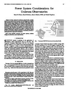
Figure 1: Performance trade-off between communication channel capacity and autonomy for net-centric sensing and observation systems
level of Intelligent Autonomy than required in most current applications of autonomous underwater vehicles, where the data collection and the control have been handled independently. On the other hand, the higher degree of autonomy provides the opportunity of significantly enhancing the overall system performance by enabling the adaptive control of the mobile nodes to take optimal advantage of the local environmental and tactical situation. This performance tradeoff between the network communication capacity and the autonomy is illustrated in Fig. 1. As illustrated schematically, the increased use of in-node intelligence or autonomy may compensate for the reduction in performance associated with the limited undersea communication channel capacity and latency. Note that the horizontal axis, representing the communication channel capacity, is labeled, with ten orders of magnitude separating the air-and land-based networks on one side and the underwater systems on the other. The vertical axis, however, is not quantified. The reason is that very little data - if any - is available in regards to quantifying the performance improvement associated with increased autonomy, and this is in fact one of the most important scientific issues associated with the development of the new distributed sensing and surveillance paradigm. For ocean monitoring and observation systems, the main mission objective for the network is the detection, classification, and tracking of episodic, often unpredictable - events. Such events include chemical plumes from undersea volcanoes or man-made systems, biological phenomena such as algae blooms. Another important application of undersea sensing systems is the detection and tracking marine mammals and man-made sources of sound in the presence of and ambient noise. 12
Without the possibility of transmitting large amounts of data back to the operators, the on-board autonomy for most such applications must be capable of fully autonomously complete the mission objective of adequately sampling and characterizing the event, without any human intervention and assistance. In addition to autonomously adapting to the environmental and tactical situation, the individual nodes may take advantage of collaboration with other nodes, again without requiring the human operator in the loop. Thus, a cluster of network nodes within - at least occasional - acoustic communication range with each other may fuse it’s own data collected for the event with those obtained by and broadcast by other network nodes in the vicinity. For example, two AUVs with acoustic arrays may each track a marine mammal and collaboratively create an accurate tracking solution by triangulation [1]. For this purpose the nodes will collect relevant, intermittent information about the event, such as the current bearing to an acoustic source, in a Contact Report, which is broadcast to the rest of the network throughout the prosecution of the event. Once the mission objectives are achieved or the autonomy decides that no more information about the event can be extracted from the data, it will broadcast an Event Report containing a compressed set of data characterizing the event. In addition to be fused with data from the rest of the network by the field control operators, the Even Report may be used by other nodes to initiate a prosecution of the event. Again such a hand-off may be performed fully autonomously without any intervention by the remote operator, and therefore not exposed to the communication latency. Such Collaborative processing and control provides yet another level of autonomy - Cluster Autonomy - with the potential of enhancing overall system performance. The local node autonomy and the cluster autonomy are to two principal levels of autonomy in the Nested Autonomy paradigm. The nesting is completed by a lower-level autonomy responsible for the actuator control and navigation on each autonomous vehicle, interfaced to the higher-level sensor-adaptive control through the “backseat-driver”, and any field level autonomy adapting the field to the larger scale environmental and tactical picture. Under support of several ONR programs over the last decade MIT has been developing a Nested, Autonomous Communication, Command and Control (NAC3 ) architecture with fully integrated acoustic sensing, modeling and control within each autonomous underwater vehicle, clusters of assets, and the entire network. The command and control architecture is highly portable and adaptable to the available acoustic communication infrastructure. Thus, the current architecture applies the Compact and Control Language (CCL) developed by Woods Hole Oceanographic institution for their Micromodem, based on 32 byte messages, with a current capacity of one point-to-point message every 20 seconds, approximately. Implemented using MOOS-IvP , the MIT NAC3 enables fully autonomous adaptation of the mobile network nodes to the environmental and tactical picture, collaborative target event by multiple platforms, and safe and efficient operation in uncharted environments, without the need for reprogramming. Thus, once deployed the entire network is operated using only the CCL messages for communication between nodes and field control and for changing mission objectives and platform states. For example, the NAC3 allows the operators to effectively control the autonomous mission behaviors to be launched by a simple set of Deploy and Prosecute commands. In the MOOS-IvP framework, the state transitions and associated vehicle behaviors initiated by the CCL commands are controlled using high-level ’behavior algebra’ in one, objective-unique mission file. In addition to a series of field experiments the development of the new Nested Autonomy NAC3 for undersea acoustic sensing is supported by a comprehensive simulation environment with highfidelity hydrodynamic and acoustic simulation for AUVs with hydrophone arrays, which allows 13
Figure 2: Nested Autonomy. The field operator is communicating with clusters of autonomous nodes through gateway assets occasionally surfacing for transmitting target reports and receiving network commands, e.g. through satellite radio communication, yielding high bandwidth, but latency of 10-30 minutes.. The nodes in the cluster communicate acoustically at low bandwidth but low latency. The Node and Cluster Autonomy are designed accordingly.
comprehensive testing of the behavior sequence, and the overall system performance. The command and control architecture has initially been developed for underwater acoustic sensing and mapping, but is currently being adapted adapted to much more general oceanographic environmental monitoring and observation systems, e.g. for command and control of mobile assets in the NSF ORION ocean observatory framework.
3
Nested Autonomy for Ocean Observation Systems
As illustrated in Fig. 1, the objective of the Nested Autonomy is to enhance the system performance beyond what is achievable by local autonomy only. This possibility is associated with the inherent layering of the communication infrastructure, with the underwater network connectivity being provided by low-bandwidth acoustic communication (ACOMMS), and the above-surface networking being provided by high-bandwidth, but latent, radio frequency (RF) communication through a 14
regularly surfacing gateway node. On-board each node, the computer bus and ethernet networking provides very high bandwidth communication between the sensing, modeling and control processes. Figure 2 shows this layered structure schematically. The vertical connectivity allows information to pass from sensors to the on-board processing and on to the control, or from each node to the field operator, and thus forms the basis for the autonomous Adaptive Control which is a key to the capability compensating for the smaller sensor apertures of the distributed nodes. Similarly, the horizontal connectivity forms the basis for Collaboration between sensors on a node (sensor fusion) or between nodes (collaborative processing and control). The three layers of horizontal communication have vastly different bandwidths, ranging from 100 byte/min for the inter-node ACOMMS to 100 Mbyte/sec for the on-board systems. Equally important, the layers of the vertical connectivity differ significantly in latency and intermittency, ranging from virtually instantaneous connectivity of the on-board sensors and control processes to latencies of 10-30 minutes for information flowing to and from the field control operators. This, in turn, has critical implication to the time scales of the adaptivity and collaborative sensing and control. Thus, adaptive control of the network assets with the operator in-the-loop is at best possible on hourly to daily basis, allowing the field operator to make tactical deployment decisions for the network assets based on e.g. environmental forecasts and reports of interfering shipping distributions, etc. Shorter time scale adaptivity, such as autonomously reacting to episodic environmental events or a node tracking a marine mammal acoustically must clearly be performed without operator intervention. On the other hand, the operator can still play a role in cuing forward assets in the path of the dynamic phenomenon, using the limited communication capacity, taking advantage of his own operational experience and intuition. Therefore, just as well as a centralized control paradigm is infeasible for such systems, it is unlikely that a concept of operations based entirely on nodal autonomy be optimal.Instead, some combination will likely be optimal, but in view of the severe latency of the vertical communication channels, the Nested Autonomy CONOPS described in the following is heavily tilted towards autonomy, as illustrated in Fig. 1. Another important effect of the layered, hybrid communication infrastructure is the significant incentive it provides for clustering assets. Thus, for example, it is more efficient to incorporate all relevant sensor types on all sensing nodes, rather than distributing the various sensing roles among different nodes, which would require communication through the slow acoustic communication channel. Similarly, the collaboration among nodes benefits significantly by deploying the fixed and mobile nodes in clusters, within each of whichthere is high probability of communication connectivity, eliminating the negative effect of the latency of the RF communication layer for communication between nodes. Thus, if the underwater assets are clustered in groups with - at least occasional - inter-node communication connectivity, such that the individual nodes may pick up event reports from other nodes, they can fuse this information with their own sensor processing to achieve an improved event tracking solution, for example. On the other hand, the environmentally induced intermittency of the underwater acoustic communication channel is well established, and it is therefore necessary that the cluster CONOPS be designed in such a manner that they are not crucially dependent on ’hand-shake’ communication between the nodes. In other words, the CONOPS must be based on the assumption that each individual node may take advantage of any target information it receives, but capable of completing the mission objective in the total absence of communication connectivity. This requirement is a key to the operational robustness and inherently makes the CONOPS autonomy-centric in contrast to the net-centric CONOPS of the land- and air-based equivalents. The CONOPS of the different layers in the Nested Autonomy 15
Figure 3: Field-level concept of operations. NaFCon field control is dispatching clusters to autonomously prosecute a chemical plume with a forecast path and expansion. Cluster A i instructed to initiate the prosecute immediately since it is closest to the projected path. The ’downstream’ Cluster B is alerted to be ready for action, while field control decides not to activate cluster C, which is not in the path of the plume.
paradigm are described in the following section.
4 4.1
Concept of Operations Field-level CONOPS
The layered and clustered NAC3 illustrated in Fig. 2 naturally leads to a nested or layered concept of operations (CONOPS), which, as mentioned earlier, provides some optimal mixture of distributed autonomy and centralized control. Figure 3 shows a possible field-level concept of operations (CONOPS) for an oceanographic observation system for capturing an episodic event, such as a chemical plume released by an undersea volcanic event. The target area is populated by a number of clusters, each with a number of mobile assets such as AUVs and gliders. One of the adaptive responsibilities of the Network and Field Control NaFCon is to deploy the finite number of clusters in a pattern which is optimal for the current environmental situation and with the highest probability for capturing the episodic event of interest. The time scales for deployment and re-deployment are are inherently long, at least of order hours, and more likely days, and is therefore highly dependent of reliable environmental and situational forecasts, often requiring a significant modeling and data assimilation infrastructure. Once deployed, it is assumed that each cluster is capable of autonomously Detecting, Classifying, 16
Figure 4: Concept of operations for cluster of AUVs with oceanographic sensors and gateway buoys for communication with NaFCon. The position and heading of a front is cued to the vehicles via the gateway buoy and they initiate a Prosecute mission, autonomously detecting the front and subsequently mapping it by zig-zagging across the frontal boundary. the two AUVs coordinate the survey to increase coverage and avoid overlap..
Localizing and Tracking the episodic event of interest. The event Prosecution may be either cued by NaFCon through a surface communication gateway, or performed fully autonomously. Once a tracking solution and the nature of the source determined, the result of the prosecution will be reported back to NaFCon in the form of an Event Report. The human operators may then cue other clusters in the projected path of the event with whatever information is available and packagable into the Compact Control Language (CCL) format suitable for transmission through the network. The final crucial role of NaFCon is the fusing of the Event Reports from the various clusters in the path of the event, gradually building up a more and more complete event track and description.
4.2
Cluster-level CONOPS
Depending on the available assets, you can envision a wide spectrum of cluster compositions, including gliders and propelled AUVs with chemical, biological and acoustic sensors. 17
Figure 4 schematically shows how such cluster assets may be applied in response to an event cuing message from NaFCon. The message identifies a front with a location and heading indicated by the dashed line. After the message is received by a surface gateway buoy, it is broadcast using the acoustic modems. Nearby nodes, e.g. a dormant, drifting or bottomed AUV, which picks up the message, will initiate a Prosecute behavior sequence, in this case the detection and subsequent mapping and tracking of a frontal boundary. Depending on the level of autonomy authorized by NaFCon, the AUV may decide not to pursue the target event if there is little probability it will come within detection range. If two or more nodes are prosecuting the event, each node may fuse the event information from the other nodes to produce a more accurate event characterization, and to optimize the coverage or resolution. Thus, in Fig. 4 the two vehicles coordinate their survey in order not to overlap and increase coverage. Another example of collaborative control is a node which did not receive the original prosecute command, but which, following the receipt of an Event Report from a prosecuting node will determine whether the target event is likely to come within range, and then autonomously initiate a prosecute sequence. All Event Reports generated by the prosecuting nodes are then collected by the communication gateway and transmitted back to NaFCon via RF communication.
4.3
Node-level CONOPS
A suite of node-level CONOPS have been developed for both single node and collaborative detection and tracking of a variety of episodic events, such as the adaptive mapping of a front or a thermocline, and for tracking an acoustic source, such as a marine mammal or a man-made source of sound. Most of these operational CONOPS have been demonstrated in a sequence of field deployments, the most recent being the Oct. 2008 GLINT’08 experiment at Pianosa Island, Italy, carried out in collaboration with NURC. As an example, Fig. 11.2 shows the core adaptive Prosecute sequence developed for the BF21 AUVs equipped with hydrophone arrays, applied for tracking an acoustic source. The numbers identifies the sequence of events involved in acoustic source prosecution sequence. 1. The AUV in this case is deployed in a low-power, continuous, hexagonal loiter pattern, awaiting commands for further action from NaFCon 2. A Prosecute message is received from NaFCon, with an estimated source location, speed and heading. 3. In response to the cuing message the AUV initiates a Search sequence, which in its simplest form closes range to the estimated track of the acoustic source. 4. Once the source signal is detected, the AUV autonomously initiates a turn maneuver which allows it to break the left-right ambiguity inherent to linear arrays. 5. Once the left-right ambiguity is resolved by the signal processing algorithm in response to the turn maneuver, the AUV will start broadcasting Contact reports containing the absolute bearing to the source, for use by any collaborating nodes and NaFCon, The AUV will then initiate the Tracking state, where it maneuvers to optimize the on-board Bearing Tracker, notably by maintaining the source at broadside, while at the same time maneuvering to 18
Figure 5: Concept of operations for single AUV with acoustic sensors autonomously Detecting, Localizing and Tracking a moving acoustic source. 1. AUV deployed in hex loiter. 2. AUV issued PROSECUTE command by NaFCon. 3. AUV entering Search state, closing range fore improving detection. 4.After detecting the source signal, the AUV enters maneuver for breaking L/R ambiguity. 5. Tracking state with AUV closing range but retaining target close to broadside. 6. Track solution achieved. 7. Classification state for source spectral characterization.
optimally produce a Source Track, i.e. a time history of the source motion, including speed and heading. In this Tracking state. the AUV may also fuse its own tracking analysis with Contact reports from other nodes in the cluster, allowing for more accurate track solution. 6. Once a satisfactory Source Track has been determined, the AUV will broadcast a Track Report for the for use by NaFCon and other nodes for fusion with equivalent information from other sensing assets to produce a more complete and accurate Global situational description.. The node CONOPS described here for the tracking of an acoustic source are directly mapped onto any other episodic event in the ocean environment, e.g. the tracking of a plume, where the collaborative, adaptive cluster autonomy is even more important by providing simultaneously the resolution and coverage required for accurately localizing, classifying and tracking the event. Thus, the network must first Detect and localize the plume, and then adaptively track its boundaries, which obviously requires the vehicles to collaborate to cover the expanding spatial extent of the plume.
19
Figure 6: Network architecture for MIT prototype of nested autonomy cluster. An arbitrary number of mobile and fixed nodes, all operated using the MOOS-IvP autonomy system architecture and backseat-driver paradigm, is connected via an underwater acoustic communication network, using a dynamically configured, generalized version of the CCL message protocol. The topside Command and Control is implemented using the same MOOS-IvP software suite, including the acoustic communication stack, situational displays, and GUIs for issuing commands to the network.
5
Cluster Autonomy System
MIT LAMS has over the last few years developed a stable prototype of a nested autonomy cluster prototype, with the architecture shown schematically in Fig. 6. An arbitrary number of mobile and fixed nodes, all operated using the MOOS-IvP autonomy system architecture and backseat-driver paradigm. Each node autonomy system is configured for its dedicated role in the network cluster through the MOOS configuration file node.moos and the IvP configuration file node.bhv. The process and behavior blocks of these configuration files are described in detail in the following chapters. The underwater nodes in the network are connected via an underwater acoustic communication network, using a dynamically configured, generalized D-CCL version of the CCL message protocol developed for the WHOI MicroModem, for which a dedicated set of MOOS.processes have been developed and extensively tested. The topside Command and Control is implemented as a MOOS community, including the acoustic communication stack. Also, the topside community incorporates a variety of situational displays, and GUIs for issuing Deploy and Prosecute commands to the network nodes . 20
6
Platform Autonomy System
The core of the nested autonomy paradigm is the autonomous, integrated sensing, modeling and control command and control framework on each individual platform. In combination with the collaborative cluster autonomy , the integrated node autonomy enables the adaptivity which may compensate for the reduced physical sensor apertures of the unmanned underwater vehicles.
6.1
The MOOS-IvP Autonomy Architecture
The Nested Autonomy paradigm for distributed undersea sensing inherently involves reaction to situations and events that are deterministically unpredictable. Thus, the autonomy architecture cannot be based on the availability of a world model that can form the basis for the autonomous decision making. Instead, it requires a capability of fully autonomously adapting to the environmental and tactical situation associated with the phenomenon is is intended to measure. As such it forms a clear example of the type of robotic system for which the Interval Programming (IvP) model for multi-objective behavior coordination was intended and developed. Thus, for example, an underwater vehicle tasked with detecting and tracking an acoustic source is faced with several, often conflicting objectives. It will likely have been assigned a station point, from which it should not move too far, while at the same time having to get close to the source to develop a reliable tracking solution. Also, depending on its sensing capability it may have a preferred heading for achieving tracking resolution. Also, if other vehicles in the vicinity is already tracking the target event, it may not be desirable for it to pursue the same source aggressively, but instead preserve power for future sensing tasks. MOOS-IvP provides exactly the flexibility and inherent multi-objective capability for implementing such high-level autonomy with adaptive and collaborative capabilities. The MOOS community used for the platforms in the MIT-LAMS implementation of the Nested Autonomy concept of operations is shown in Fig. 7. As in all MOOS communities, the MOOSDB process is the core of the MOOS architecture and handles all communication between the processes using a publish-and-subscribe architecture. The various MOOS processes include all necessary control functions as well as sensing and processing modules, with the MOOSDB providing the unified interface standard that enables the fully autonomous integration of sensing, modeling and processing, and control. MOOS ensures a process executes its “Iterate” method at a specified frequency and handles new mail on each iteration in a publish and subscribe manner. The IvP Helm runs as the MOOS process pHelmIvP. A detailed description of the role and configuration of the platform community is giving in the following.
6.2
The Back-Seat Driver Paradigm
To allow the MOOS-IvP network control to be applied on a variety of fixed and moving nodes with different control software, a “back-seat driver” paradigm was adopted and integrated with the MOOS-IvP control software infrastructure. The idea is that all high-level control, including the adaptation to measured and estimated parameters, is performed in a payload computer (PLC) running MOOS-IvP . The PLC will also handle all communication with the network, either through a radio link while surfaced, or an acoustic modem when submerged. All lower level control, and basic navigation and platform safety tasks are handled by the native vehicle control software running in the main vehicle computer (MVC), i.e. Huxley in the case of the Bluefin AUVs. The communication between the PLC and the MVC is performed over an ethernet socket,operated by a MOOS process 21
Figure 7: Unicorn MOOS Community with pHelmIvPbehavior-based autonomy module highlighted in green. All communication between processes is handled through the MOOSDB, using a mail ’publish’ and ’subscribe’ convention
pHuxley running on the PLC, as illustrated in Fig. 8. The commands passed to the MVC are simply continuous updates of desired heading, speed and depth, which the MVC then translates to desired rudder, thrust and elevator signals to the tail cone. The MVC will return current navigation and state data, which pHuxley will then publish in the MOOSDB . In the current BF’21 vehicle configuration the PLC incorporates a Linux-based CPU for general-purpose computational tasks, such as the
multi-objective helm, as well as a specialized 8 GFlop vector processor to support heavy signal processing loads such as spectrum analysis and broad-band beamforming. In this architecture, the PLC appears to the MVC as a simple NMEA device, and vice versa. (NMEA is an industry standard for communication between marine devices.) The basic safety tasks performed by the MVC include mission abort due to bottom altitude limit violations, and lack of commands from the PLC in a certain specified time, as well as an overall mission timeout. Higher level safety tasks such as exceeding the specified operating radius, and individual behavior timeouts or failures, are handled by the PLC.
6.3
Communication Connectivity
Although the concept of operation described above is autonomy centric, the communication infrastructure provides a crucial backbone of a distributed sensing and observation network. Each network node, including the sensor platforms and the communication gateways, are equipped with acoustic modems, the WHOI Micromodems. These modems implement an adaptive decision feedback equalizer with integrated Doppler and error-correction to afford 80-bps frequency hopped-FSK mode communications, and in newer implementations 5400-bps PSK mode communication. The modem provides the user with the tools necessary to create a simple time-division, multiple-access 22
Figure 8: Schematic representation of the ’back-seat driver’ paradigm, where higher level adaptive control and network communication is handled by MOOS-IvP on the payload computer, while lower level control, navigation and vehicle safety is handled by the main vehicle computer using the native control software.
(TDMA) network for master-slave polled systems, or a random-access peer-to-peer network. Each communication transaction includes a short network packet called a cycle-initialization. This specifies the source, destination and data rate of the packet to follow. A Compact Control Language (CCL) has been developed developed by Woods Hole Oceanographic Institution. In the prototype network the CCL defines a set of 32 byte messages, which are used exclusively for issuing commands to the nodes through the acoustic modem network, and for carrying sensor messages to other nodes and back to field control, including sensor status, contact and event tracking reports. Using a centralized polling scheme this communication infrastructure provides for 32 byte messages for FSK, and 2048 byte messages for PSK, being transmitted to or from a node once every minute, approximately, depending on the number of nodes in the cluster. The MOOS-IvP AC3 has been designed within this tight constraint. However, it is entirely flexible and may be straightforwardly adapted to future, higher bandwidth communication infrastructures. The interfacing of the Micromodems with the MOOS-IvP command and control infrastructure is rather complex to allow the flexibility required for the wide spectrum of mission types and objectives anticipated for an operational surveillance network.Two primary types of messages are used by the Network and Field Control (NaFCon) to provide centralized operator control; The Deploy message instructs the AUV as to where it should operate for efficient use of the field, The message includes latitude, longitude, and depth of deployment, and includes an operation radius within which it may perform autonomous., adaptive and collaboration search and mapping of episodic events. As described in the following section, the Deploy message can specify a suite of deployment mission types, depending on the mission objectives. A cluster or individual nodes may be cued by NaFCon to autonomously prosecute a target event detected and tracked by another cluster using a Prosecute message. Following the receipt of the Prosecute message, depending on the prescribed level of autonomy, the vehicle may either immediately initiate a search pattern for detecting the target event, or it may autonomously determine that the event is predicted to get within detection range before initiating the prosecution, and otherwise remain in the deployment pattern until being cued by another Prosecute Command from NaFCon, or an Event Report from another node in the same cluster indicates anh interception opportunity. 23
Figure 9: MIT BF21 vehicle states and sub-states, and state transitions for undersea acoustic source tracking. Each state is transitioned into with the receipt of a NAFCON message of the same name, with the sub-state determined by the mission type. The commands may be issued by field control or locally by the MOOS-IvP autonomy. Each state is comprised of one or more vehicle behaviors responsible for achieving the objectives of that state.
Similarly, the messages sent back to NaFCon in the acoustic source tracking prototype include a status report, including navigation data, battery state, etc., a contact report including a target bearing, and a track report providing a complete tracking solution, obviously constrained to the event information that can be packed into the CCL message.
6.4
Autonomy States and State-Transitions
The vehicle mission specification in a pHelmIvPautonomy system is comprised of a set of states for the nodes, behaviors operating in those states, and episodic, environmental or tactical events to which the node must respond. Such events include Event Reports issued by a collaborating fixed or mobile node, or target information contained in a CCL Prosecute Command from NaFCon. The states that have been defined for vehicles in an acoustic source tracking network are shown in Fig. 9. Each nodal state may have several distinct sub-states, each characterized by a set of behaviors, which based on the available navigation data, sensor input, and on-board processing results, generate objective functions for speed, depth and heading. The pHelmIvPprocess uses its multi-objective optimization algorithm to convert these objective functions into the MOOS variables DESIRED SPEED , DESIRED HEADING , and DESIRED DEPTH , which are then passed on to the lowerlevel ’front-seat’ driver control by the pHuxley MOOS process. The current behavior suite supports a total of 8 states, as shown Fig. 9, 3 of which are so-called Deploy states, and two are Prosecute states: 24
Surface State: The system initially begins in this state waiting for a Deploy message. The vehicle also autonomously returns to the Surface state message when it reaches either its return or abort waypoints. Deploy State: Entered on receipt of the Deploy Command, either received from NaFCon, or issued immediately internally once MOOS is handed over the mission control, depending on the mission file settings. The vehicle transits to its deployment location and depending on the mission type enters one of the Deploy States, shown schematically in Fig. 9. • Low-power Deploy (middle, left): This is the base-line, power-saving Deploy mode . For a vehicle with active buoyancy control this state will deploy the vehicle in a zero-speed drift at constant depth, while for a regular AUV it is typically defined as a low-speed hexagonal loiter pattern, waiting for a re-deployment or prosecute message. • Active Sensing Deploy (lower left): Here the vehicle enters a hexagonal loiter at a speed and depth that is optimal for the sensing and processing, with the acquisition and on-board signal processing active. • REA deploy (upper, center): This Rapid Environmental Assessment state is currently commanding the vehicle to perform a round-trip track-line at a certain heading while performing an adaptive vertical yo-yo pattern for mapping the thermocline. As for all other states, the actual behaviors of this state are defined in the mission file and easily changed. Prosecute State: In the Prosecute States the vehicle will actively perform an event search, localization ant tracking sequence with various levels of autonomous adaptive behavior. The Prosecute state is terminated by a Deploy Command issued autonomously if the allowed duration or operation radius is exceeded, or the tracking solution is deemed complete by the on-board processing. The Deploy location will be the current position or the assigned station point, depending on the mission configuration. Alternatively, NaFCon may issue the Deploy command. • Non-adaptive Prosecute (lower, center): This mission is a classical, non-adaptive survey pattern, such as a lawn-mower or Zig-Zag pattern, for example, depending on the settings in the behavior configuration file. Upon receipt of the Prosecute Command, the vehicle enters its survey pattern with an average heading parallel to the cued target heading. In this nonadaptive mode the breaking of left-right ambiguity and track generation is made possible by the pre-determined turns, but no adaptive behaviors are enabled. This state has no substates, since it remains in the survey pattern until the termination by the one of the state manager processes, typically pTrackQuality. • Adaptive Prosecute (middle, right): This is the core adaptive prosecute state, for the acoustic source tracking problem executing the mission sequence shown in Fig. 11.2. Depending on the level of autonomy authorized in the mission file, this state may be entered by a NaFCon - issued Prosecute Command, or it may be autonomously entered by the on-board control on a vehicle in the Active Sensing Deploy state, in response to an Event Report transmitted by another vehicle. The adaptive prosecute state has five sub-states for executing the nodal CONOPS: – Search: Currently this pre-detection state will command the vehicle on a heading that closes the range to the cued target track. If the vehicle gets within a predetermined 25
range of the estimated target position without detecting the source, it initiates a local loiter maneuver waiting for an acoustic detection. – Ambiguous: this state is entered once the source is detected and commands the vehicle to perform a sequence of turn maneuvers aimed at breaking left-right ambiguity for a linear hydrophone array. – Tracking: This is the core acoustic source tracking state, which is autonomously entered once the left-right ambiguity is resolved. The onboard processing will first stabilize the bearing tracker, after which it will initialize the tracker, and the pHelmIvPautonomy will adaptively keep the source bearing near broadside, while maintaining some attraction to the source. This behavior is continued until one of the following conditions are met: 1. Contact reports for the same target received from other nodes, which will transition the vehicle to the collaborative sub-state. 2. A stable single-bearing track solution is achieved 3. The bearing rate decreases below a threshold percentage of the maximum bearing rate achieved during the current tracking operation. 4. The deployment operation radius exceeded. 5. The vehicle is getting withing a preset minimum distance from the mission operations boundary . Except for the first condition, the vehicle will, dependent on the configuration defined in the mission file, transition to the Classify prosecute sub-state or the default Low-Power Deploy state at the current position. – Collaborative Tracking: In this sub-state the vehicle will fuse its own tracking solution with those obtained from neighbor nodes tracking the same acoustic source. Depending on the authorized level of autonomy, this state in addition to the data fusion may involve collaborative behaviors, optimizing the collaborative tracking performance. – Classifying: This is the main classification sub-state of the acoustic source prosecution, entered once a stable tracking solution has been achieved. In the current implementation the vehicle is sampling the acoustic field over a selected depth interval using a depthYoYo behavior, with a constant heading close to end-fire, to enable measurement of the vertical, angular spectrum of the acoustic field.. Abort State: The vehicle will transit toward its abort waypoint. When the waypoint is reached, a goto-surface message will be generated and the vehicle will return to the Surface state. Return State: The vehicle will transit toward its return waypoint. When the waypoint is reached, a surfacing message is generated and the vehicle will enter the Surface State. Each state is comprised of one or more vehicle behaviors responsible for achieving the objectives of that state. These behaviors are described later...
6.5
On-board, Real-time Signal Processing
A key to the autonomous, adaptive sampling of chemical, biological or acoustic fields in the ocean is an efficient on-board implementation of a data analysis package that allows for real-time feed-back to the platform control. MOOS-IvP provides a very effective infrastructure for achieving this due to its modular structure and well defined communication infrastructure. For example, for the sonar 26
payloads for the MIT AUVs, the principal processing module is the pBearingTrack. This generic beamformer and bearing tracker is applied to a wide suite of acoustic arrays operated on the AUVs. It comprises a conventional beamformer, a detection algorithm and a stabilized bearing tracker. A detailed description of these real-time acoustic processing algorithms is given elsewhere, [2], and only the functionality relevant to the autonomy shall be described here. pBearingTrack subscribes to a MOOS variable stating the availability of a new file with acoustic data. It reads the data file, performs a fourier transform and the beamformer generates a beam-time record (BTR) for the selected frequency band, which is subsequently published to the MOOSDB . A detection algorithm then determines the presence of a signal of interest, and sets a flag in the MOOSDB .. This flag is used in the mission file to identify the behaviors active in each of the sub-states, and hence controls the sub-state transitions, . Upon detection the node enters the Ambiguous sub-state, where pBearingTrack executes a algorithm that resolves the left-right ambiguity of a linear hydrophone array, executed in synchronization with a set of turn behaviors executed by the IvP Helm , as described below. Following the ambiguity resolution, the processor enters the Tracking sub-state, where the stabilized bearing tracker is used to estimate the current bearing to the source, which is continuously published to the MOOSDB for use of behaviors that optimizes the generation of an on board Target Motion Analysis (TMA), which is generated by a separate tracking module. A separate, real-time beamformer is activated in the Classification sub-state, for estimating the relative significance of shallow and steep propagation angles, which may be used as an indicator of whether the source is submerged or not.
6.6
MOOS-IvP Simulation Environment
The modular MOOS-IvP architecture directly lends itself to the establishment of a high-fidelity simulation environment. Thus, the actual mission files, and all the MOOS processes to be used for the underwater vehicle may be operated unchanged on the simulation computer, except those few processes that interact with the outside world. In the MOOS community shown in Fig. 7 the latter include the process pHuxley communicating with the main vehicle computer. In the simulator pHuxley is instead set up to communicate with a platform simulator process emulating the dynamic response of the vehicle to the helm commands for desired speed, heading and depth. Similarly, in the simulator the modem used for underwater acoustic communication is either replaced by an emulator using the actual modem hardware, or a software simulator of the modem network. The MIT MOOS-IvP simulator includes such a simulator, emulating realistic underwater communication obstacles such as propagation latency and intermittency, and message collisions. Finally, the simulator includes processes which replace the external sensors such as a CTD or an acoustic array. Thus, for example the MIT high-fidelity simulator incorporates a process for emulating CTD data collection by interpolating in a virtual ocean created by the HOPS ocean circulation model for the environment of interest. The data collected by an acoustic array are similarly emulated at the level of the the individual sensors, allowing for complete simulation of the processing chain and its feedback to and from the platform control. This feature is crucial to the development and testing of adaptive sampling behaviors.
27
Part III
MIT-LAMS Nested Autonomy Prototype 7
MOOS-IvP Nested Autonomy Architecture
Figure 10: Schematic representation of MIT MOOS-IvP Undersea Autonomous Network Architecture. The topside MOOS Community is connected to all MOOS communities on the submerged or surfaced nodes through an acoustic modem network. The network, including any number of AUV and ASC communities, is communicating using the WHOI Micromodem through the iMicroModem MOOS utility.
The network communication, command and control architecture developed and operated by the MIT Laboratory for Autonomous Marine Sensing (LAMS) is shown in Fig. 10. The topside command and control MOOS community AUV Topside, uses GUIs and the situational displays to control and command the network of fixed and mobile platforms, each operated by a MOOS community, through dedicated commands using the Compact Control Language (CCL) protocols for the WHOI Micromodem.
7.1
Sonar AUV MOOS Community
The MIT Laboratory for Autonomous Marine Sensing (LAMS) operates two Bluefin21 AUVs for research into adaptive and collaborative, autonomous acoustic sensing in the ocean. The vehicles, called Unicorn, and Caribou or Macrura depending on the configuration, can be carrying a variety of customised acoustic source/receiver payloads. In configurations for seabed object detection, classification and localization the two vehicles each have a 16-element fixed hydrophone array mounted 28
Figure 11: MIT MOOS-IvP Sonar-AUV Community: Principal MOOS-IvP modules shaded in grey, incorporating the IvP-Helm, the handlers af commands and reports communicated with field control, and onboard signal processing. The three principal interfaces to the ’outside world’ are shaded in blue: 1. The main vehicle computer (MVC) containing the ’front-seat driver’ which handles the lower level AUV navigation and control. 2. The WHOI Micromodem which handles all sub-surface network communication. 3. The sonar, consisting of a receiving hydrophone array, for active systems a source, and a control and data acquisition system (iDAS).
in the front section, and an active source for insionifying the seabed. For passive and multistatic acoustic research below 1 kHz, Unicorn is integrated with a 32-element towed hydrophone array. In either case, the vehicles are operating with MOOS-IvP handling the higher-level intelligent autonomy, implemented on a computer stack in the payload section, integrated with the acoustic source control and the data acquisition system. The MOOS-IvP configuration is shown schematically in Fig. 11. The MOOS-IvP Autonomy System is connected to the main vehicle computer using the ’back-seat driver’ paradigm, consistent with the proposed ASTM F41 standard for AUVControl. The MOOS interface to the front-seat driver is platform dependent, with several existing in the source tree, for example iHuxley for BF21 and iOEX for the Ocean Explorer. Other connections from the payload include the WHOI Micromodem, which forms the backbone of the undersea conmmunication network. The modem communication is handled by the MOOS communication stack, consisting of a generic message coder-decoder pGeneralCodec, and the pAcommsHandlerprocess handling message queueing to and from the modem driver module iMicroModem. The main purpose of the sonar payload is obviously to operate the acoustic sources and record and process data from the hydrophone array. The interface is provided by a dedicated data acquisition MOOS module iDAS (Digital Acquisition System), which interacts with the signal conditioning for each array element. iDAS subscribes for control parameters and commands from the MOOSDB, and publishes array element locations and a filename, every time a new snippet of data is available. The highbandwidth nature of the raw acoustic data makes it inconvenient to publish these directly in the MOOSDB. Instead they are written to a file, which also serves as permanent recording, and only the file location and name is published, for other processes to access, such as the signal processing 29
module, which for acoustic arrays will typically derive a bearing estimate for a source or a scatterer and publish the result in the MOOSDB for other processing such as tracking. In addition to these three main connections, there is also a process iCTD controlling and receiving data from the CTD sensor which is standard for the vehicle. Also, some of the payloads have their own GPS antenna for accurate timing, and here the MOOS interfacing is handled by the iGPS process. ¡¡¡¡¡¡¡ .mine
30
=======
31
Part IV
IvP-Helm Autonomy for Undersea Sensing 8
Mission Planning and Control
The typical mission for an AUV performing an adaptive mission involving the capture of an episodic event, such as the detection and tracking of a marine mammal, is governed by more than 30 behaviors, with each sub-state activating a dedicated suite of behaviors. All active behavior produce objective functions for desired speed, depth and heading, which the pHelmIvPprocess then combines into an optimal compromise using its interval programming, multi-objective optimization. The helm, upon startup, reads a behavior configuration file with sets of state defining conditions and mission parameters. An important component is to allow behaviors to be adaptive not only to environment events, but also to periodic direction from field control. This means a mission file is not a static script with a start and completion, but more aptly described as a state space with an initial state and conditions for migrating between states based on events; mission-control, environment or otherwise.
9
Hierarchial State Representation
An important step in the design of a MOOS-IvP autonomy system is to translate the state definitions and the transitions shown in Fig. 9 into a behavior configuration file. The newly added capability of MOOS-IvP to allow a Hierarchial State Machine (HSM) representation facilitates this process significantly, and making behavior conflicts more managable. The HSM representation of the current state definitions of the MIT sonar AUVs is shown in Fig. 12. In this form the states are shown in a hierarchial manner, with the states shown as ’parents’ and ’children’. Note that the state digram in this form does not indicate the state transitions. This is due to the fact that in the LAMS architecture, transitions are allowed between all combination states, and controlled by either the autonomy or the operators.
9.1
MOOS-IvP State Definitions
The following shows the statements in the behavior file Unicorn HSM that defines the uppermost states in Fig. 12. Listing 9.1 - MOOS-IvP State Definitions in behavior file Unicorn HSM.bhv 1 2 3 4 5 6 7 8 9 10 11 12 13
initialize DEPLOY_STATE = FALSE initialize GOTO_SURFACE = FALSE initialize PROSECUTE_STATE = FALSE // In mission or all stop on surface waiting for new deploy command set MODE = ALLSTOP { (DEPLOY_STATE = FALSE) and (PROSECUTE_STATE = FALSE) } MISSION // Diving (active mission) or surfacing (mission done) set MODE = SURFACING { MODE = MISSION GOTO_SURFACE = TRUE } DIVING
32
Figure 12: Hierarchial State Machine representation of current MIT-LAMS sonar AUV autonomy system.
14 15 16 17 18 19 20 21 22 23 24 25 26 27 28 29 30 31 32 33 34
// Deploy, Off, Return, Prosecute or Abort set MODE = DEPLOY { MODE = MISSION:DIVING (DEPLOY_STATE = DEPLOY) and (PROSECUTE_STATE = FALSE) } set MODE = OFF { MODE = MISSION:DIVING (DEPLOY_STATE = OFF) and (PROSECUTE_STATE = FALSE) } set MODE = RETURN { MODE = MISSION:DIVING (DEPLOY_STATE = RETURN) and (PROSECUTE_STATE = FALSE) } set MODE = ABORT { MODE = MISSION:DIVING (DEPLOY_STATE = ABORT) or (PROSECUTE_STATE = ABORT) } set MODE = PROSECUTE { MODE = MISSION:DIVING (PROSECUTE_STATE = PROSECUTE) and (DEPLOY_STATE = FALSE) }
Lines 1-3 initialize the state variables controlling the state definitions at mission start. The first state definition block in lines 6-8 decides whether the vehicle is inactive, state MODE=ALLSTOP, on the 33
surface, which is the initial state with the initializations in lines 1-3, or it is in a mission, controlled by the state variables DEPLOY STATE and PROSECUTE STATE. The next blocks defines whether the vehicle is actively diving, MODE=MISSION:DIVING or it is in a surfacing mode, MODE=MISSION:SURFACING, controlled by the state variable GOTO SURFACE. If in vehicle is in the active diving state, the combination of the values of the state variables DEPLOY STATE and PROSECUTE STATE define a set of mission classes. Three of these are mission terminating states, RETURN, OFF, and ABORT, while the DEPLOY and PROSECUTE states are active mission states, each with a number of sub-states as shown in Fig. 12, and described below.
9.2
Mission Terminating States
The three mission terminating states are very similar, taking the vehicle to a termination point at depth, and then surfacing. As an example, the following shows the configuration for the behaviors which become active in the RETURN state. Note that for each state there must be an active behavior producing objective functions for both speed, heading and depth. Listing 9.2 - Behavior configurations for RETURN state 1 2 3 4 5 6 7 8 9 10 11 12 13 14 15 16 17 18 19 20
Behavior = BHV_Waypoint { name = return_to_waypoint speed = 1.5 radius = 50.0 nm_radius = 100.0 updates = SENSOR_RETURN duration = no-time-limit perpetual = true condition = (MODE == RETURN) endflag = GOTO_SURFACE,TRUE } Behavior = BHV_ConstantDepth { name = return_depth updates = SENSOR_DEPTH_RETURN duration = no-time-limit condition = (MODE == RETURN) }
The following features of the behavior configuration should be noted; • The condition for activating these behaviors uses the ’==’ comparison feature of the helm, which implies that the behaviors will be active will be active in any RETURN state, irrespective of it’s place in the tree. In the present case there are no duplicate state names, but if not used, the entire tree sequence MISSION:DIVING:RETURN would have to be specified in the condition. • The return location is pecified dynamically through the updates feature, linked to the MOOS variable SENSOR RETURN, which will contain a string, gebnerated by the pNaFCon process, such as: points=1234,5432. Similarly the depth is specified dynamically through the MOOS variable SENSOR DEPTH RETURN. • Once the return location is reachede, the vehicle is transitioned into the MISSION:SURFACING state, by the endflag-specified action of setting GOTO SURFACE=TRUE. 34
The MODE=OFF state is currently identical to the RETURN state. Both the RETURN and OFF states are activated via commands from the operators, for deliberate mission termination. In contrast the ABORT state is acticvated autonomously by the autonomy system violating established system limits, such as mission duration, exceeding the opration radius, etc. The amission abort is not intantaneous, but will transition the vehicle to an abort point specified by the operator in the Deploy Command or Prosecute Command. Once the termination point is reached, and the SURFACING state is entered, the surfacing behavior is controlled by the following behavior set: Listing 9.3 - Behavior configurations for SURFACING state 1 2 3 4 5 6 7 8 9 10 11 12 13 14 15 16 17 18 19 20 21 22
Behavior = BHV_GoToDepth { name = surface_depth pwt = 100 depth = 2.5 arrival_delta = 1 perpetual = true condition = (MODE == SURFACING) // reset to ALLOFF mode, ready for new commands endflag = DEPLOY_STATE = FALSE endflag = PROSECUTE_STATE = FALSE endflag = GOTO_SURFACE = FALSE } Behavior = BHV_ConstantSpeed { name = surface_speed pwt = 100 speed = 1.5 duration = no-time-limit condition = (MODE == SURFACING) }
Note here, that when the vehicle reaches the surfacing depth, the endflag feature is used to reset the state variables to the initial values, transitioning the vehicle into the ALLSTOP state, and the vehicle will stop propulsion and drift to the surface.
9.3
Deploy States
The various Deploy modes of the nested autonomy concept of operations involve relatively simple behaviors, such as putting the vehicle into a hexagonal loiter or racetrack survey patterns. The Deploy substates are defined using the following constructs in the behavior configuration file: Listing 9.4 - MOOS-IvP Deploy State Definitions in behavior file Unicorn HSM.bhv 1 2 3 4 5 6 7 8 9 10 11 12
// Deploy States set MODE = SENSING { MODE = MISSION:DIVING:DEPLOY (DEPLOY_MISSION = 0) and (TRAIL_MACRURA = FALSE) } set MODE = LOWPOWER { MODE = MISSION:DIVING:DEPLOY DEPLOY_MISSION = 1 } set MODE = RACETRACK {
35
13 MODE = MISSION:DIVING:DEPLOY 14 (DEPLOY_MISSION = 4) or (DEPLOY_MISSION = 5) 15 } 16 17 set MODE = ZIGZAG { 18 MODE = MISSION:DIVING:DEPLOY 19 DEPLOY_MISSION = 6 20 } 21 22 set MODE = TRAIL { 23 MODE = MISSION:DIVING:DEPLOY 24 (DEPLOY_MISSION = 0) and (TRAIL_MACRURA = TRUE) 25 }
9.3.1
Loiter Sub-States
The SENSING and LOWPOWER states are currently both configured to place the vehicle in a heaxagonal loiter pattern, centered at the commanded location. The principal difference between the two states is that the SENSING has the sensors and onboard processing active, while the LOWPOWER state has them turned off for power saving. In the standard mission configurations, the vehicle is initiially placed in the LOWPOWER state using the pMessageSim module once the backseat driver autonomy is handed control. This is particularly important for AUV configurations with the modem on top, making acoustic commanding impossible at the surface. The following lists the current configuration block for the LOWPOWER state: Listing 9.5 - Behavior configurations for LOWPOWER Deploy state 1 2 3 4 5 6 7 8 9 10 11 12 13 14 15 16 17 18 19 20 21
//Basic deploy - go to loiter around deploy location Behavior = BHV_Loiter { name = deploy_loiter speed = 1.5 radius = 50.0 nm_radius = 100.0 updates = SENSOR_DEPLOY duration = no-time-limit clockwise = TRUE acquire_dist = 40 condition = MODE == LOWPOWER } Behavior = BHV_ConstantDepth { name = deploy_depth updates = SENSOR_DEPTH_DEPLOY duration = no-time-limit condition = MODE == LOWPOWER }
The loiter parameters are specified using the updates construct, using the MOOS variable SENSOR DEPLOY which will contain the location, radius and number of sides in the polygon, f.ex. polygon=radial:2000,3000,300,6, with depth specified through the variable SENSOR DEPTH DEPLOY constraining a string such as depth=25.0. Note also that all behaviors have duration=no-time-limit, remaining active as long as the mission lasts, so that each state can be entered and exited an arbitrary number of times.
36
9.3.2
Racetrack Sub-State
The racetrack substate places the vehicle in a racetrack survey pattern, typically used to create long trackline surveys. The width of the racetrack, i.e. the distance between the outgoing and incoming tracklines is specified in the behavior configuration block. In contrast to all other current Deploy States the racetrack state has several substates, depending on the depth behavior. SINGLEDEPTH: Both outgoing and ingoing tracklines at same depth, specified in SENSOR DEPTH DEPLOY. DUALDEPTH: Outgoing and ingoing tracklines at different, fixed depth, specified directly in configu-
ration block. YOYO: Depth Yoyo. ADAPTIVEYOYO: This is a special environmental sampling behavior, where the yoyo pattern is dap-
tively adjusted to sample the oceanograsphy in the vicinity of a thermocline. Used in conjunction with the pThermoTrack process, which processes the sampled oceanographic data and detects when the thermocline has been passed and then reverses the depth change. The racetrack sub-states are defined as follows in the behavior file: Listing 9.6 - MOOS-IvP State Definitions in behavior file Unicorn HSM.bhv 1 2 3 4 5 6 7 8 9 10 11 12 13 14 15 16 17 18 19 20
// Racetrack depth modes set MODE = SINGLEDEPTH { MODE = MISSION:DIVING:DEPLOY:RACETRACK (DEPLOY_MISSION = 4) and (RACETRACK_ALT_DEPTH = FALSE) } set MODE = DUALDEPTH { MODE = MISSION:DIVING:DEPLOY:RACETRACK (DEPLOY_MISSION = 4) and (RACETRACK_ALT_DEPTH = TRUE) } set MODE = YOYO { MODE = MISSION:DIVING:DEPLOY:RACETRACK DEPLOY_MISSION = 5 } set MODE = ADAPTIVEYOYO { MODE = MISSION:DIVING:DEPLOY:RACETRACK DEPLOY_MISSION = 7 }
The following shows the behavior configurations for the YOYO state: Listing 9.7 - Behavior configurations for YOYO Deploy state 1 Behavior = BHV_RaceTrack 2 { 3 name = deploy_racetrack 4 track_length = 2000 5 track_width = 0 6 distance_tolerance = 15 7 approach_angle = 60 8 heading = 270 9 speed = 1.5 10 points = 500.0, 200.0
37
11 12 13 14 15 16 17 18 19 20 21 22 23 24 25 26 27 28 29 30 31 32 33 34 35 36
updates = SENSOR_RACETRACK duration = no-time-limit condition = (MODE == RACETRACK) } Behavior = BHV_SmartYoyo { name = environmental_yoyo updates = SENSOR_YOYO min_depth = 5 max_depth = 60 min_altitude = 10 period = 300 period_segments = 200 depth_function = sinusoidal duration = no-time-limit condition = (MODE == YOYO) condition = (ON_TRACKLINE = TRUE) } Behavior = BHV_ConstantDepth { name = yoyo_approach_depth updates = SENSOR_DEPTH_DEPLOY duration = no-time-limit condition = (MODE == YOYO) condition = (ON_TRACKLINE = FALSE) }
The following features should be noted: • The BHV RaceTrack configuration block is common for all racetrack substates. • Even though fixed values are given for several parameters, the racetrack geometry is defined primarily through the use of the pHelmIvPupdates feature. Thus, the starting point of the racetrack, the trackline length, and the heading is specified in the MOOS variable SENSOR RACETRACK, containg a string such as points=2000,3000#heading=270#track length=2000. The separation of the tracklines is in this case fixed to track width=0, corresponding to the outgoing and returning tracklines being on top of each other. However, it could be included in the updates variable, obviously. The reason this is not done currently, is that the topside command console and the messsage set do not currently support the commanding of this variable. • The vertical yoyo behavior BHV SmartYoyo, described in detail in sec. ??, is similarly controlled through updates via the MOOS variable SENSOR YOYO, containing a string such as min depth=10#max depth=80. • The vertical yoyo behavior is only activated while on the trackline, flagged in the MOOSvariable ON TRACKLINE. When approaching the trackline, and during the end-turns a constant depth is instead commanded through the standard depth behavior BHV ConstantDepth. 9.3.3
ZigZag Sub-state
This behavior executes a horizontal zigzag survey at constant depth for oceanographic sampling, e.g. for mapping a frontal feature. It is non-adaptive, and the operator must specify the starting pont, the average heading and the length of the survey in the heading direction. The following shows a listing of the behavior configurations for this state. 38
Listing 9.8 - Behavior configurations for ZIGZAG Deploy state 1 2 3 4 5 6 7 8 9 10 11 12 13 14 15 16 17 18 19 20
Behavior = BHV_Waypoint { name = zigzag_mission speed = 1.5 radius = 50.0 nm_radius = 100.0 updates = ZIGZAG_STATUS perpetual = true duration = no-time-limit condition = (MODE == ZIGZAG) endflag = GOTO_SURFACE,TRUE } Behavior = BHV_ConstantDepth { name = zigzag_depth updates = SENSOR_DEPTH_DEPLOY duration = no-time-limit condition = (MODE == ZIGZAG) }
The zigzag pattern is generated by the pNaFCon process in response to the corresponding Deploy Command, with the geometry specified in the MOOS-variable ZIGZAG STATUS, containing a parameter string such as points=zigzag:5000,9000,50,1000,300,150, with the numbers represnting the starting x- and y-coordinates, the heading, the length of the survey, the period, and the amplitude. The depth is specified as for the other deploy states using the update MOOS-variable SENSOR DEPTH DEPLOY. Note that at the end of the survey, the vehicle will surface in this state. If one desires the vehicle to return to the the LOWPOWER loiter state, f.ex., line 11 should simply be replaced by endflag = DEPLOY MISSION = 1. 9.3.4
Trail Sub-state
This is a new autonomy state that was first demonstrated in the GLINT’08 experiment. In this state, the vehicle will perform synchronized swimming with another vehicle. This is achieved by constantly extrapolating the location and speed of the other vehicle, using the Status Reports received over the acoustic modem. If communication is lost to the other vehicle for a duration exceeding a specified time, the vehicle will enter a local loiter pattern until communication is re-established, and the pursuit can be resumed. The following shows the behavior configurations for this state. Listing 9.9 - Behavior configurations for TRAIL Deploy state 1 Behavior = BHV_Trail 2 { 3 name = trail_macrura 4 contact = MACRURA 5 trail_range = 300 6 trail_angle = 315 7 trail_angle_type = absolute 8 radius = 10 9 nm_radius = 100 10 max_range = 1000 11 decay = 60,180 12 13 condition = (MODE == TRAIL)
39
14 15 16 17 18 19 20 21 22 23 24 25 26 27 28 29 30 31 32 33 34 35 36 37 38 39 40 41 42 43
condition = (MACRURA_NAV_SPEED >= 1.0) runflag = TRAILING = TRUE idleflag = TRAILING = FALSE activeflag = ACTIVE_TRAIL = TRUE inactiveflag = ACTIVE_TRAIL = FALSE } Behavior = BHV_Loiter { name = trail_idle_loiter pwt = 100 speed = 1.4 radius = 50.0 nm_radius = 100.0 updates = SENSOR_DEPLOY center_activate = true duration = no-time-limit clockwise = FALSE acquire_dist = 40 condition = (MODE == TRAIL) condition = (ACTIVE_TRAIL = FALSE) } Behavior = BHV_ConstantDepth { name = trail_depth updates = SENSOR_DEPTH_DEPLOY duration = no-time-limit condition = (MODE == TRAIL) }
The following features should be noted: • This state uses a newly added set of flags to switch from the trailing mode to an idle loiter state in cases where communication is lost, or the trailed vehicle is moving below a certain speed, e.g. when it surfaces for GPS. The activeflag and inactiveflag parameters are used to specify MOOS-variable settings indicating whether the behavior is generating an objective function or not. Thus, when the conditions keep the trail behavior form generating an objective function, it will flag this by setting ACTIVE TRAIL=FALSE in the MOOSDB, and the idle loiter behavior will become active until the flag is reversed, and the pursuit will be resumed. • The trail in this case is set to an absolute bearing from the contact. • Since the current command set does not allow for specifying thye trail distance and bearing angle, these must be set to fixed values in the behavior file.
9.4
Prosecute States
A major challence is the execution of the autonomous Prosecute mission, involving all the components of the completely autonomous strategy for the capturing and characterizing the event in question. The Prosecute substates are defined using the following constructs in the behavior configuration file: Listing 9.10 - MOOS-IvP Prosecute State Definitions in behavior file Unicorn HSM.bhv
40
1 2 3 4 5 6 7 8 9 10 11 12 13 14 15 16 17 18 19 20
// Prosecute Missions set MODE = SEARCH { MODE = MISSION:DIVING:PROSECUTE TRACKING = NO_TRACK } set MODE = AMBIGUOUS { MODE = MISSION:DIVING:PROSECUTE TRACKING = AMBIGUOUS } set MODE = TRACKING { MODE = MISSION:DIVING:PROSECUTE TRACKING = TRACKING } set MODE = CLASSIFYING { MODE = MISSION:DIVING:PROSECUTE TRACKING = CLASSIFYING }
9.4.1
Search Sub-State
The initial Search prosecute sub-state is entered upon receipt of a Prosecute Command from NaFCon. Entering this state, a suite of behaviors optimizing the propability of detection of the event are activated, synchronized with the modules processing the sensor data. Irrespective of the nature of the event, theSearch state involves two behaviors that provide a trade-off between closing range to the cued event location and requirements for station-keeping. By dynamically assigning priorities to these behaviors, the autonomoy system may allow the cluster to automatically dispatch the vehicles closest to the event to be more actively pursuing the event by using available information about the positions of other assets in the cluster. The BHV Attractor behavior, described in Sec. 10.1, uses the MOOS-IvP CPA engine to attract the vehicle towards the Closest Point of Approach (CPA) for the projected event track. Inside a mininimum predicted range, the priority is set to zero, basically turning off the attractor behavior. This feature is used in connection with remote sensing missions using optical or acoustical sensors. The objective of keeping the vehicle in the vicinity of its assigned station point is handled by the IvP behavior BHV RubberBand, described in detail in Sec. 10.2. This behavior is a ’soft’ version of the standard station-keeping IvP behavior, pulling the vehicle back towards its assigned station point.once it exceeds a range set in the configuration file. Outside this range, the priority is linear with distance, similar to the elasticity of a rubber band, hence the name. The priority of these two competing behaviors can either be fixed or dynamically determined by a command and control process, such as pClusterPriority, for example, based on the relative distances of the cluster assets to the target event. By setting the relative valus of the RubberBand and Attractor behaviors, the system designer may control the relative importance of prosecuting an event and maintain stationkeeping. In a cluster configuration with several vehicles, these priorities may be set dynamically using the general IvP UPDATES parameter. Thus, to avoid all vehicles in a cluster chasing the same target, the priorities may be set dynamiclly to favorize the assets closest to the projected target track, with ’down-stream’ assets not abandoning the target but instead gaining priority with time in case the closer assets miss the detection opportunity. The balancing of these priorities is the Cluster Autonomy, the next level of the Nested autonomy. Also, while the concept has been developed for the tracking of single target event, this is no inherent limitation. 41
The handling of multiple targets depends on the capabilty of the signal processing module and the availability of a process handling the Contact Management, the subject of future developments. Depending on the mission objectives, other behaviors may be added. For example, for improving detection of an acoustic source in an anisotropic noise field, the noise interferrence may be minimized using certain array orientations. The standard behavior configuration block for the SEARCH state is Listing 9.11 - Behavior configurations for Prosecute SEARCH state 1 2 3 4 5 6 7 8 9 10 11 12 13 14 15 16 17 18 19 20 21 22 23 24 25 26 27 28 29 30 31 32 33 34 35 36 37 38 39 40 41 42 43 44 45 46 47 48
Behavior = BHV_Attractor { name = search_attract updates = MY_TARGET priority = 100 duration = no-time-limit condition = (MODE == SEARCH) condition = IN_RANGE,FALSE contact = TGT_1 dist_priority_interval = 1000,2000 strength = 1.0 decay = 1800,3600 patience = 50 } Behavior = BHV_RubberBand { name = search_rubberband updates = DEPLOY_STATION priority = 100 duration = no-time-limit condition = (MODE == SEARCH) condition = IN_RANGE = FALSE inner_radius = 500 outer_radius = 500 outer_speed = 1.5 stiffness = 0.5 } Behavior = BHV_ConstantDepth { name = search_depth updates = SENSOR_DEPTH_DEPLOY duration = no-time-limit condition = (MODE == SEARCH) } Behavior = BHV_Loiter { name = search_loiter speed = 1.5 radius = 50.0 nm_radius = 100.0 updates = PROSECUTE_LOITER duration = no-time-limit clockwise = TRUE acquire_dist = 40 condition = (MODE == SEARCH) condition = IN_RANGE,TRUE }
The following features should ne noted • The MOOS-variables MY TARGET is used to dynamically assign a specific target ID to the attractor behavior, as well as the desired priority, f.ex. contact=TGT 6#priority=156. 42
• The DEPLOY STATION is used are used to define the currently assigned deploy station. • The IN RANGE flag indicates whether the vehicle is inside a specified range of the expected target track, without yet having made a detection. If IN RANGE=TRUE the vehicle will go into a waiting pattern, here a loiter pattern, until the event is detected, or the prosecute mission is timed out. The loiter may of course be replaced by any other behavior which improves the detection probability. Thus, for detecting a chemical plume or an upwelling event, a traditional ocean search behavior, such as an expanding spiral survey may be applied. 9.4.2
Ambiguous Sub-State
Once an event is detected, the node enters the Ambiguous sub-state, where the onboard signal processing in corncert with dedicated maneuvering will attemt to break any sensing ambiguities. Examples of sensing ambiguities include the direction of a detected ocean front, which must be determined to autonomously decide on a mapping survey strategy, and the left/right ambiguity of the bearing from an acoustic array to a source. For the source tracking problem using a linear hydrophone array, the onboaard processor, e.g. pBearingTrack, will determine the relation between a forced array turn and the associated change in source bearing. A behavior controlling the change in array heading is BHV HArrayTurn. If the sensing is unambiguous, this state is simply never entered by the onboard processing, and the system is transitioned directly into the TRACKING or CLASSIFYING states. The following shows the behavior configurations for the acoustic source tracking problem Listing 9.12 - Behavior configurations for Prosecute AMBIGUOUS state 1 2 3 4 5 6 7 8 9 10 11 12 13 14 15 16 17 18 19 20 21 22 23
Behavior = BHV_ConstantDepth { name = ambiguous_depth updates = SENSOR_DEPTH_DEPLOY duration = no-time-limit condition = (MODE == AMBIGUOUS) } Behavior = BHV_HArrayTurn { name = ambiguous_arrayturn turn_angle = 120 pwt = 700 condition = (MODE == AMBIGUOUS) } Behavior = BHV_ConstantSpeed { name = ambiguous_speed speed = 1.5 duration = no-time-limit condition = (MODE == AMBIGUOUS) }
Note that as in all other states, there must be behaviors generating objective functions for both speed, heading and depth. Since no specific depth is currently set for the prosecute, the desired depth is simply inherited from the previous deploy command, through the updates variable SENSOR DEPTH DEPLOY.
43
9.4.3
Tracking Sub-State
Once the ambiguity is resolved by the on-board signal processing, it sets the sub-state flag to TRACKING, andthe helm will enter the Tracking sub-state, activating behaviors which maneuvers the vehicle to optimize the tracking of the target event.. There are currently three Tracking Sub-states defined for the undersea sensing autonomy system. In addition to the principal, adaptive event prosecution, the behavior set also allows the nodes to perform more conventional surveys in response to the Prosecute Command, such as a horizontal zig-zag along a frontal bounday. ADAPTIVE This is the principal, adaptive state for optimally track an acoustic source, or a tar-
get for active sonar applications. The behaviors in this state defines a platform maneuvering which weighs the various mission oblectives and constraints against a configuration which optimizes tracking performance. The active behaviors in this state include the BHV Attractor and BHV RubberBand behaviors also used in the Search sub-state, but not necessarily with the same relative priority. Thus, once the acoustic source is detected and the ambiguity resolved, the vehicle should likely be allowed to increase the priority of the attractor behavior and reduce the importance of the station keeping. Also, the safety behaviors, such as collision avaoidance behaviors, obviously remain active. All of these behaviors will be competing with the principal tracking behavior, BHV HArrayAngle, with the relative significance controlled by the assigned priority weights. If authorized in the configuration, an adaptive sub-mode, MULTIPLE will allow the vehicle to fuse source bearing information from collaborating nodes for generating an improved track solution. If no Contact Reports are received from other nodes, the system will instead be in the SINGLE state, where it will maneuver to optimize a single vehicle track solution. To optimize collaborative tracking dedicated behaviors may be activated in the MULTIPLE state. HEX In this non-adaptive state the vehicle will enter a standard hexagonal loiter patter, with sensing
and processing active. TMA This state will execute the classical Target Motion Analysis zigzag survey with a heading
commanded from the topside command and control. In this non-adaptive mode the node will use the IvP Helm behavior BHV ZigZag to perform the survey, in a direction defined by a heading stated in a dedicated MOOS variable. In this non-adaptive mode this heading must be defined by the operator, e.g. based on oceanographic forecasts or intuition. These tracking sub-states are defined as follows in the behavior file: Listing 9.13 - Tracking Substate Definitions in behavior file Unicorn HSM.bhv 1 2 3 4 5 6 7 8 9 10 11 12
// Adaptive Prosecute states set MODE = ADAPTIVE { MODE = MISSION:DIVING:PROSECUTE:TRACKING PROSECUTE_MISSION r2 ), and simply “shadowing” the contact(r < r1 ). The default is r1 = 5 and r2 = 15. The assocoated priority transition is controlled by the STRENGTH parameter as shown in Fig. 13. GIVEUP RANGE: The distance (in meters) that the contact must be within for the behavior to be
active and produce an objective function. The default giveup range value is zero, making the behavior active active regardless of the distance to the contact. PATIENCE: This parameter controls the ’patience’ of the vehicle in chasing the target. The default is
0, which forces the vehicle to immidiately head for the contact, even if the contact is approaching and cutting range on its own. This parameter is useful when poaer conservation is critical, and when the vehicle is required to stay close to a station point (zone defense) DECAY: This parameter takes two arguments separated by a comma. The first argument is the
decay start time (in seconds), and the second is the decay end time (also in seconds). The behavior extrapolates the contact position based on the last known position, heading and speed. The speed of the contact begins to decay based on the time since the last contact update. This is a safeguard against perpetually trailing a vehicle that ceases to provide a contact report. The default is 5 and 10 seconds respectively. For undersea networks with acoustic communication only, 60-120 seconds would be a reasonable choice. Listing 10.1 - An example BHV Attractor configuration. 0 1 2 3 4 5 6 7 8 9
Behavior = BHV_Attractor { name = bhv_trail pwt = 100 contact = delta strength = 0.5 priority_interval = 100,200 patience = 50 decay = 20,60 }
10.1.1
MOOS variables subscribed to by BHV Attractor:
. MOOS variable
Type
Description
Published by
NAV X
D
Ownship UTM x-coordinate
pHuxley
NAV Y
D
Ownship UTM y-coordinate
pHuxley
NAV SPEED
D
Current vehicle speed in m/s
pHuxley
NAV HEADING
D
Current ownship heading in degrees
pHuxley
’contact’ NAV X
D
UTM x-coordinate of contact
pTransponderAIS
’contact’ NAV Y
D
UTM x-coordinate of contact
pTransponderAIS
’contact’, NAV HEADING D
Current contact heading in degrees.
pTransponderAIS
’contact’ NAV SPEED
D
Current contact speed in m/s.
pTransponderAIS
’contact’ NAV UTC
D
UTC time of latest contact report
pTransponderAIS
48
Figure 14: Range-dependent priority of BHV RubberBand.
. 10.1.2
MOOS variables published by BHV Attractor:
. MOOS variable
10.2
Type
Description
Format
ATTRACTOR RELEVANCE D
Computed relevance in % of objective function. Published at integer precision
50
. ATTRACTOR RANGE TO CONTACT
Range to attracting target in meters. lished at integare precision
1500
D
Pub-
BHV RubberBand
This behavior is very similar to BHV StationKeep, but has a range-dependent priority, such that the restoring force back towards the station point is increasing with distance similarly to a rubber band attached to the station point. It keep the vehicle at a given lat/lon or x,y position by varying the speed to the station point as a linear function of its distance to the point. The parameters allow one to choose the two distances between which the speed varies linearly between 0 at the inner radius and the value of the parameter OUTER SPEED at the outer radius. Also, the priority is increasing linearly betwen the two radii, and outside the outer radius, the priority is increasing linearly with a rate specified by the parameter STRENGTH, as illustrated in Figure 14. The following parameters are defined for this behavior: STATION PT: The x,y position of the point upon which to station keep. It is a comma separated
pair of numerical values. INNER RADIUS: The radius from the station point within which the behavior takes no action to
affect the vehicle position. 49
The radius from the station point within which the behavior does take action to affect the vehicle position. It produces an objective function as if the station point were a waypoint. The desired speed varies linear between the INNER RADIUS and the OUTER RADIUS, approaching zero at the inner radius and the speed given by OUTER SPEED at the outer radius.
OUTER RADIUS:
The desired speed varies linear between the INNER RADIUS and the OUTER RADIUS, approaching zero at the inner radius and the speed given by OUTER SPEED at the outer radius.
OUTER SPEED:
STRENGTH: If the vehicle is outside the outer radius, the priority will increase linearly with distance
by this rate. Listing 10.2 - An example BHV RubberBand configuration. 0 Behavior = BHV_RubberBand 1 { 2 name = bhv_rubber_band 3 station_pt = 50,75 4 inner_radius = 3 5 outer_radius = 15 6 outer_speed = 2.2 7 extra_speed = 2.2 8 condition = ON_STATION = true 9 condition = RETURN = false 10 }
10.2.1
MOOS variables subscribed to by BHV RubberBand:
. MOOS variable
Type
Description
Published by
NAV X
D
Ownship UTM x-coordinate
pHuxley
NAV Y
D
Ownship UTM y-coordinate
pHuxley
10.2.2
MOOS variables published by BHV RubberBand:
. MOOS variable
Type
Description
Format
STATION CIRCLE
$
Status message
1000,2000,10,bobby
DIST TO STATION
D
Distance to station point in meters. Published at integer precision
1200
50
11
Undersea Adaptive Sensing Behaviors
11.1
BHV HArrayTurn
Used for breaking left/right ambiguity inherent to linear hydrophone arrays, this behavior will perform a sequence of clockwize and anti-clockwize turns until the signal processing module has declared that the bearing ambiguity is resolved. If this is not happening before the heading has changed by a specified amount, the behavior will switch to turning up to the same angle in the opposite direction, and so on until the ambiguity is resolved. The configuration parameters for BHV HArrayTurn are as follows. TURN ANGLE: The angle the array will be turned for breaking ambiguity before reversing direction.
Listing 11.1 - Example BHV HArrayTurn configuration 1 Behavior = BHV_HArrayTurn 2 { 3 name = ambiguous_arrayturn 4 turn_angle = 120 5 pwt = 700 6 condition = (MODE == AMBIGUOUS) 7 }
11.1.1
MOOS variables subscribed to by BHV HArrayTurn:
. MOOS variable
Type
Description
Published by
NAV X
D
Ownship UTM x-coordinate
pHuxley
NAV Y
D
Ownship UTM y-coordinate
pHuxley
AEL HEADING
D
Current mean heading of hydrophone array
pAEL
TRACK STAT
$
Tracking state vector
p1HTracker
11.1.2
MOOS variables published by BHV HArrayTurn:
. None.
11.2
BHV HArrayAngle
The bearing resolution of a linear acoustic array is best at broadside, and to optimize the bearing track solution produced by the signal processing module pBearingTrack, it is desirable to keep the acoustic source near broadside, as illustrated in Fig. . This behavior maintains controls the desired heading to keep the array heading, published in the MOOS variable AEL HEADING , near broadside. This also aids the creation of a Source Track solution because it in general will create a curved path of the array. Because this behavior competes against the other acttive behaviors, notably the attractor behavior, the resulting array angle will be tilted towards forward endfire, but this in effect is also beneficial to the tracking since the closer the vicinity of the target, the more curvature of the vehicle path will result. The configuration parameters for BHV HArrayAngle are as follows. 51
The desired angle in dgrees between the hydrophone array and the estimated source direction as reported in the MOOS variable BEARING STAT. Forward endfire corresponds to 0◦ , and backward endfire to 180◦ . The behavior creates a symmetric objective function, and the rusulting heading depends on which of the two optimal heading is closest to the current heading, and other active behaviors, such as BHV Attractor, for example.
DESIRED ANGLE:
Listing 11.2 - Example BHV HArrayAngle configuration 1 Behavior = BHV_HArrayAngle 2 { 3 name = track_array_angle 4 pwt = 100 5 width = 60 6 desired_angle = 90 7 condition = (MODE == ADAPTIVE) 8 }
MOOS variables subscribed to by BHV HArrayAngle:
11.2.1 .
MOOS variable
Type
AEL HEADING BEARING STAT
11.2.2
Description
Published by
D
Current mean heading of hydrophone array
pAEL
$
Bearing tracker status vector
pBearingTrack pBearingsSim
MOOS variables published by BHV HArrayAngle:
. None.
11.3
BHV SmartYoyo
This behavior adapts a vertical yoyo with specified horizontal period to the current water depth, as illustrated in Figure 15. By covering the entire water column in the survey, this behavior is also extremely useful for collecting oceanographic information. It provides for accurate control of the depth changes. Thus, the vertical survey pattern can be either linear or sinosoidal, with a controlled period and a specified number of discrete depth intervals. It will attempt to maintain a constant depth in each segment, which is useful for averaging a sensing parameter at each selected depth. In the current MIT-LAMS autonomy system, this behavior is used in the environmental sampling YOYO state using large number of segments and a relatively short range period, and in the CLASSIFY state with few discrete depths and a longer range period. The configuration parameters for the BHV SmartYoyo behavior are as follows. MIN DEPTH: Upper turning depth in meters. MAX DEPTH: Lower turning depth in meters. MIN ALTITUDE: Minimum altitude in meters. Depth yoyo will be consistently scaled to yield a lower
turning depth which does not get closer to the bottom than this value. 52
Figure 15: BHV SmartYoyo. This behavior adapts a vertical yoyo with specific horizontal period in distance traveled to the current water depth. May be combined with arbitrary horizontal behaviors, such as loiter and zigzag.
PERIOD: Horizontal length of one full period of depth yoyo in meters. PERIOD SEGMENTS: Number of depth segments within a yoyo period. The desired depth will be held
constant withing each segment. DEPTH FUNCTION: Shape of depth function. Choices are linear and sinusoid. Note that the actual depth profile will depend on the number of period segments as well.
Listing 11.3 - Example BHV SmartYoyo configuration 1 Behavior = BHV_SmartYoyo 2 { 3 name = classify_yoyo 4 min_depth = 10 5 max_depth = 60 6 min_altitude = 5 7 period = 1200 8 period_segments = 10
53
9 depth_function = linear 10 duration = no-time-limit 11 condition = (MODE == CLASSIFYING) 12 }
MOOS variables subscribed to by BHV SmartYoyo:
11.3.1 .
MOOS variable
Type
Description
Published by
NAV DEPTH
D
Current vehicle depth in meters
pHuxley
NAV SPEED
D
Current vehicle speed in m/s
pHuxley
NAV ALTITUDE
D
Current altitude above bottom in meters
pHuxley
IN TRACK
$
Logical indicating whether vehicle is on desired survey track (TRUE), our ourside, e.g. turning (FALSE). Yoyo is only active if TRUE, otherwize depth will be held constant.
BHV RaceTrack
11.3.2
MOOS variables published by BHV SmartYoyo:
. None.
11.4
BHV ZigZag
This behavior creates a horizontal zigzag survey, initiated at the position the behavior becomes active. It is defined by a mean heading, period, and amplitude, as depicted in Fig.16. The functional shape of the survey can be either a sawtooth pattern (linear) or a sinusoid. The horizontal survey pattern may be combined with any depth behavior. . The configuration parameters for the BHV ZigZag behavior are as follows. PERIOD: Horizontal period in meters. AMPLITUDE: Amplitude of zigzag i meters. HEADING: Heading in degrees of zigzag baseline. ZIGZAG FUNCTION: Shape of zigzag function. Choices are linear and sinusoid.
Listing 11.4 - Example BHV ZigZag configuration 1 Behavior = BHV_ZigZag 2 { 3 name = dlt_zigzag_survey 4 speed = 1.5 5 updates = PROSECUTE_HEADING 6 period = 600 7 amplitude = 150 8 heading = 135 9 zigzag_function = linear 10 duration = no-time-limit 11 condition = (MODE == TMA) 12 }
54
Figure 16: BHV ZigZag: This behavior produces a horizontal zigzag survey along a specified mean heading and speed. May be combined with arbitrary vertical behaviors, such as constant depth or yoyo.
MOOS variables subscribed to by BHV ZigZag:
11.4.1 .
MOOS variable
Type
Description
Published by
NAV X
D
Ownship UTM x-coordinate
pHuxley
NAV Y
D
Ownship UTM y-coordinate
pHuxley
11.4.2
MOOS variables published by BHV ZigZag:
. None.
11.5
BHV RaceTrack
Although any horizontal survey pattern can be generated using standard behaviors, such as BHV Waypoint, a dedicated racetrack behavior has been designed that emphasises a well defined trackline and a 55
controlled trackline approach. Also, this behavior will publish a flag indicating whwther the vehicle is on or outside the desired trackline, which is used for limiting the periodic surfacings for GPS to happen only during turns at the end of the tracklines. It will generate a survey composed of two parallel tracklines, separated by a specified distance, which may be set to zero for the two tracklines being identical. The configuration parameters for the BHV RaceTrack behavior are as follows. TRACK LENGTH: Length of the outgoing and returning tracklines in meters. TRACK WIDTH: Separation of the outgoing and returning tracklines in meters. DISTANCE TOLERANCE: Allowed deviation from the trackline in meters, beyond which the trackline
will be approached at the specified approach angle. Inside this distance the approach angle will be exponentially decreasing towards the trackline. . APPROACH ANGLE: Approach angle in degrees towards the trackline, with zero being parallel to the
trackline, applied outside the tolerance distance. Should typically be set to 45-60 degrees to produce effective trackline following. HEADING: Absolute heading in degrees of trackline. SPEED: Vehicle speed in m/s. TRACK LENGTH: Length of the outgoing and returning tracklines in meters. POINTS: UTM x- and y-coordinates of racetrack starting location, comma separated.
Listing 11.5 - Example BHV RaceTrack configuration 1 Behavior = BHV_RaceTrack 2 { 3 name = deploy_racetrack 4 track_length = 2000 5 track_width = 0 6 distance_tolerance = 15 7 approach_angle = 60 8 heading = 270 9 speed = 1.5 10 points = 500.0, 200.0 11 updates = SENSOR_RACETRACK 12 duration = no-time-limit 13 condition = (MODE == RACETRACK) 14 }
11.5.1
MOOS variables subscribed to by BHV RaceTrack:
. MOOS variable
Type
Description
Published by
NAV X
D
Ownship UTM x-coordinate
pHuxley
NAV Y
D
Ownship UTM y-coordinate
pHuxley
56
11.5.2
MOOS variables published by BHV RaceTrack:
. MOOS variable
Type
Description
Format
IN TRACK
$
Logical indicating whether vehicle is inside the survey track range(TRUE), our ourside, e.g. turning (FALSE).
TRUE FALSE
ON TRACKLINE
$
Logical indicating whether vehicle is considered on the trackline, i.e. less than distance tolerance from the ideal trackline (TRUE), our ourside, e.g. approaching trackline (FALSE).
TRUE FALSE
57
¿¿¿¿¿¿¿ .r639
Part V
Autonomous Communication, Command and Control 12
MOOS-IvP Communication, Command and Control
Figure 17: MOOS-IvP community for MIT sonar AUVs, with the autonomous communication, command and control modules highlighted in gold.
The Autonomous Communication, Command and Control components of the MOOS-IvP autonomy system handles the communication between the payload autonomy system, including the autonomous Helm, and the outside world. The communication with the main vehicle computer “front-seat driver” is handled by the pHuxley process, responsible for passing desired speed, heading and depth as desired by the Helm to the main vehicle computer, which is then responsible for translating these commands into actuator actions. The MVC responds back with navigation information, which is then published in the MOOSDB for use by other modules, including the autonomy helm pHelmIvP. The connection with the topside field control operators is performed using the acoustic modems, with the so-called Communication Stack handling the coding/decoding (CoDec)message scheduling, and modem transmission and reception. Both of these interfaces are controlled by the AC3 handler process, pNaFCon, which is responsible for translating command messages from the topside operators into state variables for the inboard autonomy system, and for translating the current vehicle states into status reports for broadcasting 58
to the network. Similarly, the state of the vehicle is translated into commands for the “front-seat driver”, such as disabling and enabling the “back-seat driver” control. A number of other processes are integrated into the prototype autonomy system for managing the state transitions in accordance with the nested autonomy CONOPS. A list of autonomous communication, command and control processing modules is given in Table 1. A more detailed description is given in the following.
12.1
Node Level Command and Control
In the Nested Autonomy paradigm the node level Command and Control is highly tilted towards autonomy, with the vehicle actions being defined by the current vehicle state and the associated behavior set, and the sensor input. The possibility of the cluster and the field control to alter the node behavior is limited to simple, higher level commands, the only role of which is to transition the vehicle to another, allowed state. Thus, for example, if the NaFCon operators want to alter the vehicle behavior during a prosecute mission, their only option is to transition the vehicle to another allowed state, defined in the configuration file. The detailed actions such as heading, speed and depth of the node are not directly controllable by the operators. For example, the operators have the power to override an active prosecute mission by transmitting a Deploy Command or switching the node to an alternative Prosecute State. Similarly, the state of the node may be altered by other nodes in the cluster only if allowed in the mission configuration on the node. For example, in the MIT Nested Autonomy Prototype, the process pTargetOpportunity will react to incoming Track Reports by issuing itself a Prosecute Command if the target is predicted to come within an allowed perimeter.
12.2
Cluster Level Command and Control
Depending on the CONOPS, the control of the Cluster may be performed either centrally from NaFCon, by a ’leader node’ in the cluster controlling the states of the ’cluster team’, or fully distributed. A team sports analogy of the centralized control is American football, with its reliance on real-time communication infrastructure. In contrast, team sports such as basketball and soccer rely on each individual player making decisions based on his own situational awareness, strategy and tactics. In the MIT Nested Autonomy Prototype the fully distributed option has been chosen, in large part because of the high level of autonomy made available by the IvP Helm , and the latent and intermittent undersea communication infrastructure. An example of the distributed cluster control is the Synchronized Swimming activated in the TRAIL sub-state. Here the trailing vehicle will use the BHV Trail behavior to maintain a fixed relative or absolute bearing, and range to a collaborating node, simply by monitoring the status reports it broadcasts. Because of the latency and intermittency, the extrapolation feature of the trail behavior is crucial to the performance. Another important feature is a limit on the validity of the messages received from the other vehicle. Thus, if the collaborating node has not been heard from for a specified time, the extrapolation of its position will be ignored, and the trailing node will enter a local loiter behavior until a fresh status report from the other vehicle is received, and the trailing resumed. Another distributed cluster control feature of the prototype is the collaborative search and tracking behaviors activated in response to a Prosecute Command. Again these behaviors are car59
#
Module Name
Module Description
Author
1
pNaFCon
Manages translation of commands from field control to autonomy state, and conversely translates autonomy state to status reports. Manages “back-seat driver” control Libraries: mbutil, MOOS, MOOSGen, MOOSUtility
Balasuriya
2
pMessageSim
Used to make initial deploy of vehicle in cases where acoustic communication is not applicable on surface. Optionally makes prosecute command as well. Libraries: mbutil, MOOS, MOOSGen, MOOSUtility
Eickstedt
3
pSearch
State transition manager for acoustic source tracking CONOPS. Responsible for managing the transition into the Prosecute State in response to a Prosecute Command. Re-deploys if target not interceptable. Libraries: MOOS, MOOSGen, MOOSUtility
Eickstedt
4
pTrackQuality
State transition manager for acoustic source tracking CONOPS. Responsible for terminating the Prosecute State. Also issues redeploy before vehicle reaches operational limits for all states. Libraries: MOOS, MOOSGen, MOOSUtility
Schmidt
5
pTargetOpportunity
State transition manager for acoustic source tracking CONOPS. Transitions autonomously from Deploy to Prosecute State. Monitors incoming Track reprorts and issues Prosecute Command to ownship if target can be intercepted Libraries: MOOS, MOOSGen, MOOSUtility
Schmidt
6
pClusterPriority
This process weights the priority to track a target (using BHV Attractor) by how close the vehicle is to the target relative to all the collaborating nodes. Closer vehicles are given higher weights, thus leading to a “zone defense” style of multivehicle autonomy. The last piece to this “zone defense” scheme is the BHV RubberBand, which attracts vehicles back to their initial deploy location which increasing strength with distance. Libraries: tes util, mbutil, MOOS, MOOSGen, MOOSUtility
Schneider
7
pHuxley
Does something Libraries: MOOSUtility
Balasuriya
8
pGeneralCodec
Highly extensible encoder / decoder of messages from human readable integers, booleans, strings, or floats to hexidecimal strings suitable for sending by the WHOI MicroModem. Libraries:tes util, MOOS, MOOSGen, MOOSUtility
Schneider
9
pAcommsHandler
Manages queues for transmission of acoustic messages. Different message queues can be given priorities that increase with time since the last message was sent from that queue. Libraries: tes util, MOOS, MOOSGen, MOOSUtility
Schneider
10
pAcommsPoller
Manages and schedules polling of other nodes on the modem network. Libraries: tes util, MOOS, MOOSGen, MOOSUtility
Schneider
11
iMicroModem
Driver process for WHOI micromodems. Libraries: tes util, MOOS, MOOSGen, MOOSUtility
Grund
mbutil,
MOOS, MOOSGen,
Size
Total unique lines of code Total aggregate lines of code Table 1: Autonomous Communication, Command and Control Modules for MOOS-ivP onboard autonomy system.
60
ried out without any need for two-way handshake communication with the other cluster nodes. The paradigm philosophy is that any useful information from other nodes is fused into the situational awareness, but the individual nodes are not dependent on any outside information for pursuing the mission objective. A characteristic example is the dynamic, distributed assignment of priorities of the cluster behaviors BHV Attractor and BHV RubberBand, with the first attempting to attract the node towards the cued target position and the other trying to maintain the node near the assigned station point. In the sports analogy, the command and control process pClusterPriority implements an autonomous zone defense strategy by dynamically assigning priorities based on the known position of the other cluster assets and the cued target position. Without requiring any explicit coordination and communication with the other nodes, each node will therefore on its own assign priority to the two competing behaviors. As a result, the cluster node closest to the target will most aggressively initiate pursuit. On the other hand, the other nodes are not sitting idle, but pursuing the target with some finite priority, thus ensuring that they are in a position to more actively initiate the search in case the closest node fails to detect the target or never reacted because it did not receive the cuing message. Again, the soccer analogy is obvious, with all defenders moving in position to react if a forward from the other team is passing by the first line of defense. The actual behaviors associated with this distributed ’zone defense’ is never commanded directly, but built into the relative priorities of the competing behaviors allocated by pClusterPriority. Based on a large number of virtual and field experiments a range-exponential priority allocation appears optimal. In addition to the cluster command and control components of the on-board processing also adopts the distributed decision paradigm. For example, the fusion of bearing tracks received from other platforms are applied on collaborating nodes if deemed useful, e.g. for producing a georeferenced target track (pMBTracker), but the nodes are not dependent on it, and will continue to attempt a single node tracking sequence (p1HTracker) if it does not receive useful information from other nodes.
12.3
Field Level Command and Control
Although a large amount of autonomous command and control is delegated to the nodes the field level operators obviously have the ultimate control authority with the power to change the roles of the various clusters and nodes under its command. However, in the Nested Autonomy paradigm this authority can only be exercised through simple commands that trigger a state transition on the network nodes. The ultimate action associated with the issued commands is entirely defined in the MOOS-IvP configurations on the nodes. The commands for the network nodes are encoded into Compact Control Language (CCL) messages which are then transmitted via the acoustic modem network infrastructure. In the PLUSNet prototype a limited message set was hard coded into a couple of dedicated CCL messages. This message set was very restrictive, allowing only a handful of state transitions. Thus, to enable a certain Deploy or Prosecute mode in was necessary to change the configuration files before the vehicle was deployed. To allow an arbitrarily large state space to be activated without recovery and re-configuration, an new message handler, coder and decoder stack was developed in 2008 by Toby Schneider at MIT. Most of the stack was tested successfully in the August 2008 GLINT’08 experiment. The new software stack was completed in the fall of 2008 with the development of the completely generic coder-decoder (CoDec) pGeneralCodec. it uses a dedicated CCL message,
61
assigned number 32, with a highly flexible message format that allows for optimal compression and content, specified in a configuration file which may be changed to optimally fit the specific geographical region and mission suite. The configuration files for the MIT Nested Autonomy Prototype are descried in Appendix A. In an actual operating system the command and control CCL messages may be generated either by the operators directly, or by a topside command and control autonomy system, e.g. linked to an environmental forecasting framework. In the MIT prototype the commands are issued by the operator, typically the Chief Scientist or a trained pilot using the topside MATLAB GUI, NaFConSim.m. In combination with the new CCL software stack, it allows the operators to a activate any of the autonomy states without reconfiguration. The NaFConSim GUI is currently configured for issuing Deploy Commands with 7 allowed Mission Types: 0 Transitions the node to the SENSING state, in the current configuration a hexagonal loiter with the on-board sensing and processing active. 1 Transition to LOWPOWER state. In the prototype a hexagonal loiter around the deploy location. 2 Transition to OFF state. Currently the vehicle transits to the deploy location and surfaces. 3 Transition to RETURN state. In the prototype identical to the OFF state. 4 Transition to RACETRACK state. In prototype configuration the vehicle will run a zero-width racetrack at the specified heading and length, starting at the deploy location. 5 Transition to YOYO state. In prototype the vehicle will run the same racetrack as for mission 4, but executing a vertical YoYo survey using the BHV SmartYoyo behavior. 6 Transition to ZIGZAG state. Similarly, the GUI is configured for selecting 4 Prosecute Mission Types. All the mission types initially transitions to the SEARCH state, followed by the AMBIGUOUS state once the cued target event is detected. Once the ambiguities are resolved. the node will transition into one of the TRACKING sub-states, depending on the mission type, 1. Transition to ADAPTIVE tracking state, where the vehicle will adaptively maneuver to optimize the tracking performance. 2. Same as 1, but once tracking is deemed satisfactory by the pTrackQuality process, it will enter the CLASSIFYING state, which in the prototype will maintain a heading pointing towards the computed target track. 3. Transition to TMA state, where the vehicle in the prototype will enter a zig-zag survey along a specified heading. 4. Transition to a hexagonal loiter similar to the one used in the SENSING Deploy Mission.
62
As mentioned earlier, the number of Deploy and Prosecute commands the communications stack can handle is unlimited. The current suite is dictated only by the capabilities built into the GUI. Thus for example, the TRAIL state used for Synchronized Swimming can currently only be activated by changing the configuration, e.g. by replacing one of the other deployment modes. This and other useful transitions will be enabled in the next release of the topside command GUI.
63
13
Communication, Command and Control Modules
13.1 13.1.1
pNaFCon Brief Overview
pNaFCon is the MOOS process that provides the connectivity between the network communication infrastructure and the autonomy states of the vehicle. As such it is the principal link between the communication infrastructure and the pHelmIvP behavior-based autonomy. Thus, it subscribes to the command messages from the topside and status and contact reports from other nodes and performs the associated state transitions by posting a set of state variables. Thus for example, in response to a topside Deploy Command the MOOS variables DEPLOY STATE is published by pNaFCon to place the vehicle in its Deploy state, with DEPLOY MISSION defining the deploy sub-states, such as a low-power drift, a loiter pattern, or an environmental sampling mission with a YoYo in depth along a horizontal racetrack. Similarly, pNaFCon publishes the variables PROSECUTE STATE and PROSECUTE MISSION to transition the vehicle autonomy into a particular Prosecute sub-state, such as adaptive target tracking or a traditional TMA ZigZag survey, for example. NaFCon also is responsible for generating Status and Contact reports, depending on the state of the vehicle. Thus, for example it will respond to a target bearing being published by the real-time data processing by creating a contact Report message, which will then be queued, scheduled and transmitted bythe acoustic communication stack.
13.1.2
Parameters for the pNaFCon Configuration Block
The following configuration parameters are defined for pNaFCon. ProsecuteMission: Default rosecute mission: 1: Adaptive DLT; 2: Adaptive DLT with subsequent depth-discremination clasification. This parameter used to be necessary since the pFramer CoDec
used until recently did not allow more than a single type of Prosecute mission to be commanded via the acoustic link. When using the new generic CoDec pGeneralCoDec this parameter is obsolete and will be eliminated in future versions. etc etc Below is an example configuration block for pNaFCon, Listing 13.1 - An example pNaFCon configuration block . 1 2 3 4 5 6 7 8 9 10 11 12 13 14 15
/////////// Global Variables //////////////// LatOrigin = 36.87 LongOrigin = -122.42 MagneticOffset = 0.0 ////////Configuration Block for pNaFCon /////////////// ProcessConfig = pNaFCon { AppTick = 4 CommsTick = 4 ProsecuteMission = 1 DestinationPlatformId = 3 CollaboratingPlatformId = 4 TrackId = 31 Orbit_radius =300 Orbit_points = 6
64
16 ZigZag_Period = 300 17 ZigZag_Amplitude = 150 18 Report_Delay = 2; 19 }
The LatOrigin and LonOrigin parameters on lines 1-2 are not specific to pNaFCon, but are specified at the global level in a MOOS file. They are needed to allow the conversion between local x-y coordinates and latitude-longitude coordinates. They are mandatory parameters and pNaFCon will refuse to launch if they are lacking - but they are mandatory for other common MOOS applications as well. 13.1.3
MOOS variables subscribed to by pNaFcon:
. MOOS variable
Type
Description
Published by
NAV X
D
Local UTM x-coordinate for ownship
pHuxley
NAV Y
D
Local UTM y-coordinate for ownship
pHuxley
NAFCON MESSAGES
S
Incoming acomm messages
13.1.4
MOOS variables published by pNaFCon:
.
65
MOOS variable
Type
Description
Format
DEPLOY STATE
$
Defines DEPLOY state.. “FALSE”: Vehicle not in DEPLOY state “OFF”: Vehicle is idleing “DEPLOY”: Vehicle in DEPLOY state “ABORT”: Vehicle transiting to abort point
MICROMODEM COMMAND
$
Polling a Collaborating node
POLL REQUEST
D
Poll request flag
COLLABORATOR ID
$
Collaborating id from moos file
SINCE POLLED
D
Time since last poll
BEARING STAT
D
Initialize BEARING STAT = 0
REMOTE COLLABORATION
D
State of the collaborating node ”OFF”: No collaboration ”SYNCH”: In synch ”COLLABORATING”: In collaborating mode
COMMUNITY STAT
$
Status of the collaborating vehicle
BEARING STAT2
$
Contact info. of the collaborating vehicle
TRACK STAT2
$
Track info. of the collaborating vehicle
GOTO SURFACE
$
Goto surface flag ”TRUE” or ”FALSE”
DEPLOY STATION
$
Station keeping position
TARGET ID
$
Track number for prosecuted target
5
TARGET STATE
$
Cued target location and source characteristics for use by target simulators
tgt x=2000, tgt y=1525, ..... tgt id=5
TGT id NAV X
$
Cued UTM x coordinate for id’th target
TGT id NAV Y
$
Cued UTM y coordinate for id’th target
TGT id NAV HEADING
$
Cued Heading of id’th target
TGT id NAV SPEED
$
Cued speed id’th targets
TGT id NAV UTC
$
UTC time of cued target info
MY TARGET
$
Current target of interest
CURRENT TARGET
$
Current target id
PLUSNET MESSAGES
$
Status and contact messages to be broadcast by modem
66
TGT 5
13.2
pMessageSim
13.2.1
Brief Overview
This MOOS module provides an automated procedure for launching a vehicle into an initial Deploy state at some specified delay following launch. It does so by simply posting a NAFCON MESSAGES in the MOOSDB in the same way as pNaFCon. It is particularly useful in cases where the conditions do not support the launching via the acoustic modem. In fact it was originally written by D. Eickstedt at sea in the MB06 trial in Montery Bay, where the communication stack was not yet robust enough to provide reliable cammanding of the vehicles. pMessageSim also provides the optional launching of a delayed Prosecute command to the vehicle itself. After the acomms stack has become further developed, this option is rarely used. 13.2.2
Parameters for the pMessageSim Configuration Block
The following configuration parameters are defined for pNaFCon. message type: Deploy mission type. Action depends on settings in behavior configuration file.
Current mission suite is 0 Continuous DCL hex-loiter deployment: Sensors and processing turned on 1 Low-power deployment. 2 Off. Go to surface 3 Return to station and surface 4 Environmental mission. Racetrack 5 Evironmental mission. Adaptive vertical yoyo. Horizontal racetrack 6 Environmental mission. Horizontal zigzag, constant depth. trigger depth: Depth at which delay timer for deploy message is triggered. If negative triggering
will occur at start-up.. deploy delay: Delay in seconds of deploy message. If not specified, default is 30 seconds. prosecute delay: Delay in seconds of prosecute message. In most cases set to value larger than
mission time to disable autonmatic prosecute message. deploy x: UTM x-coordinate of deployment point. deploy y: UTM y-coordinate of deployment point. deploy depth: Depth of deployment. dest addr: Destination platform ID. Here Ownship vehicle ID. abort x: UTM x-coordinate of abort point. When aborting the vehicle will transit to this point at
depth and then surface.. 67
abort y: UTM y-coordinate of abort point. abort depth: Depth at which vehicle will transit to abort point. op radius: Operations radius allowed for vehicle relative to current deploy location. If deploy command issued to a location outside this range, the state manager process, currently pTrackQuality,
will issue a local deploy. deploy duration: Duration in seconds of deploy state. If exceeded without redeploy, vehicle will enter ABORT state and transit to abort location and surface. target x: UTM x-coordinate of target to be prosecuted after PROSECUTE DELAY. target y: UTM y-coordinate of target to be prosecuted. target depth: Depth of target to be prosecuted. target heading: Heading of target to be prosecuted. target speed: Speed of target to be prosecuted. target id: Identification number allocated to target to be prosecuted. prosecute duration: Duration in seconds of prosecute state. If exceeded without redeploy, vehicle will enter ABORT state and transit to abort location and surface. yoyo distance: Length of racetrack legs for Deploy Mission 4 and 5, and length of zigzag projection
on average heading for Deploy Mission 6. yoyo heading: Heading of racetrack legs for Deploy Mission 4 and 5, and average heading for Deploy
Mission 6. yoyo upper: Upper turning depth of vertical yoyo. yoyo lower: Lower turning depth of vertical yoyo.
Below is an example configuration block forpMessageSim, Listing 13.2 - An example pMessageSim configuration block . 1 2 3 4 5 6 7 8 9 10 11 12
/////////// Global Variables //////////////// LatOrigin = 36.87 LongOrigin = -122.42 MagneticOffset = 0.0 ////////Configuration Block for pMessageSim /////////////// ProcessConfig = pMessageSim { AppTick = 4 CommsTick = 4 message_type = 1 trigger_depth = -1
68
13 prosecute_delay = 60000 14 deploy_x = 5000 // 500 A6 racetrack 15 deploy_y = 9000 // 2100 A6 racetrack 16 deploy_depth = 25.0 17 dest_addr = 3 18 abort_x = 4500 19 abort_y = 8500 20 abort_depth = 6.0 21 op_radius = 5000 22 deploy_duration = 7200 23 target_x = 0 24 target_y = 1000 25 target_depth = 20.0 26 target_heading = 90.0 27 target_speed = 2.0 28 target_id = 5 29 prosecute_duration = 1800 30 yoyo_distance = 4000 31 yoyo_heading = 135 32 yoyo_upper = 5 33 yoyo_lower = 30 34 }
The LatOrigin and LonOrigin parameters on lines 1-2 are not specific to pMessageSim, but are specified at the global level in a MOOS file. They are needed to allow the conversion between local x-y coordinates and latitude-longitude coordinates. They are mandatory parameters and pMessageSim will refuse to launch if they are lacking - but they are mandatory for other common MOOS applications as well. 13.2.3
MOOS variables subscribed to by pMessageSim:
. MOOS variable NAV DEPTH
13.2.4
Type D
Description
Published by
Current ownship depth. message
Used fro triggering
pHuxley
MOOS variables published by pMessageSim:
. MOOS variable NAFCON MESSAGES
Type $
Description
Format
Deploy or prosecute message for ownship.
69
13.3 13.3.1
pSearch Brief Overview
pSearch is a transition manager for the transition from Deploy State to Prosecute State in response to a Prosecute Command issued either by NaFCon , pMessageSim or the target watchdog process pTargetOpportunity described later. Once a NAFCON MESSAGES command is reived from the MOOSDB, pSearch will first detemine whether the target is interceptable within the specified distance. If not, it will return the vehicle to its earlier Deploy State. If the target is interceptable it will continuously monitor the target and ownship motion, checking for continued interceptability. If the minimum distance to the expected target position is reached with detection, pSearch will enter a local loiter pattern iwth the sensors remaing active for possible detection of the target event.
13.3.2
Parameters for the pSearch Configuration Block
min range: Range from predicted target position at which vehicle will enter waiting loiter pattern
until possibly detecting the target event. orbit radius: Radius applied in waiting loiter hexagon awaiting possible event detection giveup range: Target range in meters beyond which the prosecute will not be pursued. Vehicle
will remain in or return to Deploy State Below is an example configuration block forpSearch, Listing 13.3 - An example pSearch configuration block . 1 2 3 4 5 6 7 8 9 10 11 12 13 14
/////////// Global Variables //////////////// LatOrigin = 36.87 LongOrigin = -122.42 MagneticOffset = 0.0 ////////Configuration Block for pSearch /////////////// ProcessConfig = pSearch { AppTick = 4 CommsTick = 4 min_range = 500 orbit_radius = 300 giveup_range = 2500 }
13.3.3
MOOS variables subscribed to by pSearch:
.
70
MOOS variable
Type
Description
Published by
VEHICLE ID
D
Node number for ownship.
pNaFCon
NAV X
D
Ownship UTM x-coordinate
pHuxley
NAV Y
D
Ownship UTM y-coordinate
pHuxley
PROSECUTE STATE
$
Prosecute state
pNaFCon
TARGET STATE
$
Assumed target state vector from Prosecute Command
pNaFCon
SENSOR DEPLOY
$
Current Deploy location
pNaFCon
SENSOR DEPTH DEPLOY$
Current Deploy depth
pNaFCon
DEPLOY RADIUS
D
Maximum operating radius in meters
pNaFCon
ABORT LAT
D
Abort location latitude in decimal degrees
pNaFCon
ABORT LONG
D
Abort location longitude in decimal degrees
pNaFCon
ABORT TIME
D
UTC Abort time
pNaFCon
SENSOR DEPTH ABORT D
Depth ofr transit to abort location
pNaFCon
TRACKING
Tracking state. Indicates whether target has been detected or not.. “NO TRACK”: No detection yet “AMBIGUOUS”: Detection, but ambiguous bearing “TRACKING”: Un-ambiguous bearing tracking “CLASSIFYING”: Classifying sub-state
pBearingTrack
13.3.4
$
MOOS variables published by pSearch:
. MOOS variable
Type
Description
Format
NAFCON MESSAGES
$
Deploy for ownship published if the intercept conditions for a reported target are satisfied.
. TRACK STAT
$
Comma separated track state vector. Initializes to state=0. If target not detected the target state variable is set to state=4.
node=3,state=0,x=...
IN RANGE
$
Flag indicating whether vehicle is within minimum range to expected target position.
TRUE FALSE
71
13.4 13.4.1
pTrackQuality Brief Overview
This is the principal autonomus state transition managing process responsible for terminating the Prosecute State for acoustic source tracking missions. It is monitoring a suite of MOOS variables and performs state transitions accordingly. It’s main objective is to terminate a source tracking Prosecute Mission, and return the vehicle to its default Deploy State. The transition is triggered either by the tracking solution with satisfactory uncertainty being achieved, or the maximum number of Track Reports is reached. pTrackQuality is also monitoring the distance to the boundaries of the operations box and the distance from the station point, and will issue a redeploy if too close, to avoid the Surfacing triggered by the helm if the boundary is exceeded. This feature is active in both the Deploy and Prosecute states. 13.4.2
Parameters for the pTrackQuality Configuration Block
bearing rate threshold: If positive sets the threshold for terminating source tracking. When
bearing rate decreases below the set percentage of the max imum bearing rate. Can produce undesired terminations if set too high. Rarely used. track limit: Maximum duration of Tracking Sub-State in seconds. When exceeded, vehicle will be
re-deployed. min opbox distance: Minimum allowed distance to operations box boundary. Triggers re-deploy
when reached to avoid ’hard’ abort by Helm. max classify time: Maximum duration of Classify Sub-State of source tracking prosecute in sec-
onds. When exceeded, vehicle will be re-deployed. track sigma single: Standard deviation threshold for single vehicle track solution in meters. TRACK REPORT will be issued when computed standard deviation is less than this value. buffer length single: Number of single vehicle track solutions used in computing track uncer-
tainty. track sigma multiple: Standard deviation threshold for multi-vehicle, collaborative track solution in meters. TRACK REPORT will be issued when computed standard deviation is less than this value. buffer length multiple: Number of multi-vehicle, collaborative track solutions used in computing
track uncertainty. track report time: Duration of time period where Track Reports are issued. When exceeded,
vehicle will transition to Deploy State. deploy location: Location of re-deploy. Can be ither ’station’ or ’present’, for return to station
point or preset position, respectively.
72
Below is an example configuration block forpTrackQuality, Listing 13.4 - An example pTrackQuality configuration block . 1 2 3 4 5 6 7 8 9
/////////// Global Variables //////////////// LatOrigin = 36.87 LongOrigin = -122.42 MagneticOffset = 0.0 ////////Configuration Block for pTrackQuality /////////////// ProcessConfig = pTrackQuality { AppTick = 1 CommsTick = 1
10 11 12 13 14 15 16 17 18 19 20 }
bearing_rate_threshold = 0 track_limit = 600 min_opbox_distance = 500 max_classify_time = 600 track_sigma_single = 100 buffer_length_single = 10 track_sigma_multiple = 100 buffer_length_multiple = 3 track_report_time = 180 deploy_location = station
// // // //
percent of max achieved during tracking Tracking duration in seconds min distance to opreg perimeter max Classify time for PROSECUTE_MISSION = 2
// Options: station or present
The LatOrigin and LonOrigin parameters on lines 1-2 are not specific to pMessageSim, but are specified at the global level in a MOOS file. They are needed to allow the conversion between local x-y coordinates and latitude-longitude coordinates. They are mandatory parameters and pMessageSim will refuse to launch if they are lacking - but they are mandatory for other common MOOS applications as well. 13.4.3
MOOS variables subscribed to by pTrackQuality:
.
73
MOOS variable
Type
Description
Published by
VEHICLE ID
D
Node number for ownship.
pNaFCon
TGT # NAV X
D
UTM x-coordinate of target. Initially from Prosecute Command. Updated by tracking solution
pNaFCon p1HTracker pMBTracker
TGT # NAV Y
D
UTM x-coordinate of target. Initially from Prosecute Command. Updated by tracking solution
pNaFCon p1HTracker pMBTracker
TGT # NAV UTC
D
UTC time of target location
p1HTracker pMBTracker
NAV X
D
Ownship UTM x-coordinate
pHuxley
NAV Y
D
Ownship UTM y-coordinate
pHuxley
SENSOR DEPLOY
$
Current Deploy location
pNaFCon
SENSOR DEPTH DEPLOY$
Current Deploy depth
pNaFCon
PROSECUTE STATE
$
Prosecute state
pNaFCon
PROSECUTE MISSION
$
Prosecute mission type
pNaFCon
BEARING STAT
$
Comma-separated bearing state variables: vehID,state,bearing,x,y,beamno,sigma,utc
pBearingTrack
TRACK STAT
$
Tracking state vector
p1HTracker
TRACKING
$
Tracking state. “NO TRACK”: No detection yet “AMBIGUOUS”: Detection, but ambiguous bearing “TRACKING”: Un-ambiguous bearing tracking “CLASSIFYING”: Classifying sub-state
pBearingTrack
TRACKING MODE
$
Tracking mode: “SINGLE”: Single vehicle tracking “MULTIPLE”: Multi-vehicle cross-bearing tracking
pMBTRacker
CLOSE RANGE
$
Reset flag for geo trackers
pSearch
CLASS DONE
$
Flag set to TRUE when classification substate is completed.
pTrackQuality
. DEPLOY RADIUS
D
Maximum operating radius in meters
pNaFCon
OPREG TRAJECTORY PERIM DIST
D
Current distance to operations box in meters
pHelmIvP
ABORT LAT
D
Abort location latitude in decimal degrees
pNaFCon
ABORT LONG
D
Abort location longitude in decimal degrees
pNaFCon
ABORT TIME
D
UTC Abort time
pNaFCon
Depth ofr transit to abort location
pNaFCon
SENSOR DEPTH ABORT D
74
13.4.4
MOOS variables published by pTrackQuality:
. MOOS variable
Type
Description
Format
NAFCON MESSAGES
$
Deploy for ownship published if any of the prosecute termination conditions are satisfied.
. TRACK REPORT
$
Track Report issued when uncertainty satisfactory. Translated into modem message by
pNaFCon TRACKING
$
Tracking substate flag. Changed to “CLASSIFYING” if PROSECUTE MISSION = 2 and tracking is satisfactory
CLASS DONE
$
Flag set to TRUE when classification substate is completed.
.
75
13.5
pTargetOpportunity
13.5.1
Brief Overview
pTargetOpportunity is a transition manager that autonomously transitions from Deploy State to Prosecute State if a Track Report is received from a collaborating vehicle for an event, such as an acoustic source or a plume, is heading in a direction that allows ownship to intercept. It currently represents the highest level of autonomous decisionmaking on the vehicle. When a Track report is received from the collaborting vehicle the closest point of approach is calculated, and the prosecute command will be issued only if the CPA is les than a maximum range specified in the configuration file. There are currently one of two algorithms apllied, dependent on the compiler settings. The ultimate one uses the standard MOOS-IvP CPA engine, but this algorithm needs debugging. The other uses a simple minimum distance computation ignoring the estimated target speed. At this point both set of configurationj parameters are specified.
13.5.2
Parameters for the pTargetOpportunity Configuration Block
CollaboratorNodes: Comm-separated list of vehicle ID for trusted collaborator nodes. Only Track
Reports from nodes on the list will be acted upon. OpportunityMission: Prosecute Mission to be applied:
1. Adaptive tracking mission 2. Adaptive tracking with subsequent classification sub-state 3. Zig-Zag mission at estimated target heading 4. Loiter deploy pattern ith tracking. OpportunityRadius: Minimum target distance, below which a Prosecute Command is issued to
ownship. VehicleMaxSpeed: Maximum estimated speed of target to be intercepted ThresholdCPA: Threshold range for CPA below which a prosecute sequence will be initiated ThresholdTOL: Tolerance of the CPA determination.
Below is an example configuration block forpTargetOpportunity, Listing 13.5 - An example pTargetOpportunity configuration block . 1 2 3 4 5 6 7 8 9
/////////// Global Variables //////////////// LatOrigin = 36.87 LongOrigin = -122.42 MagneticOffset = 0.0 ////////Configuration Block for pTargetOpportunity /////////////// ProcessConfig = pTargetOpportunity { AppTick = 4 CommsTick = 4
76
10 11 12 13 14 15 16 17 }
CollaboratorNodes = 0,4 OpportunityMission = 1 OpportunityRadius = 2000 VehicleMaxSpeed = 2.0 ThresholdCPA = 1000 ThresholdTOL = 20
The LatOrigin and LonOrigin parameters on lines 1-2 are not specific to pMessageSim, but are specified at the global level in a MOOS file. They are needed to allow the conversion between local x-y coordinates and latitude-longitude coordinates. They are mandatory parameters and pMessageSim will refuse to launch if they are lacking - but they are mandatory for other common MOOS applications as well.
13.5.3
MOOS variables subscribed to by pTargetOpportunity:
. MOOS variable
Type
Description
Published by
VEHICLE ID
D
Node number for ownship.
pNaFCon
COLLABORATOR ID
D
Node number for collaborating vehicle
pNaFCon
NAV X
D
Ownship UTM x-coordinate
pHuxley
NAV Y
D
Ownship UTM y-coordinate
pHuxley
NAV DEPTH
D
Current ownship depth in meters
pHuxley
DEPLOY STATE
$
Deploy state
pNaFCon
PROSECUTE STATE
$
Prosecute state
pNaFCon
TRACK STAT2
$
Tracking state vector received from collaborating vehicle
pNaFCon
DEPLOY RADIUS
D
Maximum operating radius in meters
pNaFCon
OPREG TRAJECTORY PERIM DIST
D
Current distance to operations box in meters
pHelmIvP
ABORT LAT
D
Abort location latitude in decimal degrees
pNaFCon
ABORT LONG
D
Abort location longitude in decimal degrees
pNaFCon
ABORT TIME
D
UTC Abort time
pNaFCon
Depth ofr transit to abort location
pNaFCon
SENSOR DEPTH ABORT D
13.5.4
MOOS variables published by pTargetOpportunity:
. MOOS variable NAFCON MESSAGES
Type $
Description
Format
Deploy for ownship published if the intercept conditions for a reported target are satisfied.
.
77
13.6 13.6.1
pClusterPriority Brief Overview
This MOOS module does a darn good job at doing what it is supposed to do 13.6.2
Parameters for the pClusterPriority Configuration Block
The following configuration parameters are defined for pClusterPriority. verbose: Level of diagnostic verbosity during runtime. Choises are verbose, terse, and quiet. target: Name of target prosecuted by the cluster. Can be fixed, e.g. TGT 6 or BOBBY. If speci-
fied to ’target updates’ the target identification is dynamically allocated. The MOOS variable containing the dynamical target ID is specified in the configuration parameter target updates. target updates: Identifies the MOOS variable containiing the ID for the target currently being prosecuted. If not specified default is TARGET ID. behavior updates: Identifies the MOOS variable used for publishing the behavior updates, e.g. for use by BHV Attractor. If not specified default is MY TARGET. ownship: Node ID for ownship, case insensitive, e.g. UNICORN. friend: Node ID for collaborating cluster node, case insensitive, e.g. CARIBOU. Must be specified
for each cllaborating node. pwt: Base priority weight for attracting behavior, e.g. BHV Attractor. max delay friends: Maximum allowed delay in seconds for status reports recveived from collabo-
rating nodes. If exceeded the node will be ignored in computing attractor priorities. Below is an example configuration block for pClusterpriority, Listing 13.6 - Sample pClusterPriority configuration block . 1 ProcessConfig = pClusterPriority 2 { 3 AppTick = 4 4 CommsTick = 4 5 verbosity = verbose 6 target = target_updates 7 target_updates = TARGET_ID 8 behavior_updates = MY_TARGET 8 ownship = unicorn 9 friend = macrura 10 friend = OEX 11 pwt = 100 12 max_delay_friends= 60 13 }
13.6.3
MOOS variables subscribed to by pClusterPriority:
. 78
13.6.4
MOOS variables published by pClusterPriority:
.
79
13.7 13.7.1
pHuxley Brief Overview
pHuxley is the process which interface with the Main Vehicle Computer (MVC-Huxley) of the Bluefin AUV. During start up pHuxley requests the data streams required from the MVC. Once the backseat driver is turned on (i.e. when the front-seat driver (MVC) is ready to receive commands from the back-seat) a flag is set and pHuxley starts sending desired speed, heading and depth values to the MVC. pHuxley controls the hand-offs between the front-seat and the back-seat.
13.7.2
Parameters for the pHuxley Configuration Block
13.7.3
MOOS variables subscribed to by pHuxley:
. 13.7.4
MOOS variables published by pHuxley:
.
80
pHelmIvP
CTD Display
Higher Level Processes
pGeneralCodec pBTRCodec
pCTDCodec
pAcommsHandler iMicroModem
Encoding/Decoding Level
Message Queuing Modem Driver
MOOSDB Acoustic Communications 80 bps - 5400 bps
MicroModem
Figure 18: schematic of current acoustic modem stack
13.8 13.8.1
pGeneralCodec Brief Overview
Any terms in italics are defined the Glossary (section 13.8.9). Problem Communication between multiple autonomous vehicles is often subject to severe throughput limitations, especially in the ocean environment, where highly rate-limited acoustic channels are often the only option. In order to make the best use of this available bandwidth, messages need to be compacted to a minimal size before sending. Background Figure 18 illustrates the current status of the acoustic communication software “stack” from the viewpoint of this laboratory. pGeneralCodec fits in the level of message encoding/decoding, as suggested by the name. Solution pGeneralCodec is an process that proposes to be a practical first-pass solution to the difficult problem posed here. It reduces the data required to be sent by: • Predefined messages: the user must specify a message structure what specifies what fields the message contains and how large each field should be (in an intuitive fashion that pGeneralCodec turns into bits). Both the sender and receiver have preshared knowledge of the message structure. From this knowledge, no meta information about the message (beyond an identifier) needs to be sent, simply the data. • Custom field sizes: message fields are defined with custom tolerances (ranges and precisions) that are tighter than those given by the IEEE standards for floating point and integer numbers. For example, if a field needs to hold an integer that will never range outside [0, 1000] that field in the message will only be 10 bits long (ceil(log2 1001)). Furthermore, pGeneralCodec has powerful parsing abilities for both encoding and decoding, including the ability to perform certain geodesic conversions (latitude, longitude ↔ UTM x,y) and lookups (modem id ↔ vehicle name) on data. 81
13.8.2
Parameters for the pGeneralCodec Configuration Block
Example .moos file The moos file is simple since the bulk of the configuration is stored in separate XML files (see section 13.8.5 for the configuration of these files): //-----------------------------------------------------------------// pGeneralCodec configuration block ProcessConfig = pGeneralCodec { // available to all moos processes. AppTick = 4 CommsTick = 4 // available to all tes moos processes //verbose, terse, quiet verbosity = verbose message_file = example1.xml message_file = example2.xml message_file = bobs_special_command_set.xml }
Filling out the .moos file • verbosity: choose verbose for full text terminal output, terse for symbolic heartbeat output, and quiet for no terminal output. • message_file: path to an XML file containing a message set of one or messages. 13.8.3
MOOS variables subscribed to by pGeneralCodec:
All the variables subscribed to by pGeneralCodec are configured within the message XML files. See section 13.8.5 and beyond for details on filling out and interpreting these XML files. Thus, in the following table instead of MOOS variables, XML tags from the message XML file are listed. For each defined, a subscription takes place for the MOOS variable specified at run time within the tag. For example, the .moos file includes a file message_file = example1.XML, and example1.XML contains the tag STATUS_HEX_30B. Thus, STATUS_HEX_30B is subscribed for.
82
XML tag specifying MOOS variable
a
Description
Published by
$
Hexadecimal string to decode (probably from MicroModem).
pAcommsHandler MOOSBlink)
$ or D
Contains the modem id to send this message from. Can either be double (ex: 3) or string (ex: ...,destkey=3,...)
pNaFCon (PLUSNET MESSAGES) or others
$ or D
A publish here triggers the creation of this message. The contents may contain message parts or not.
pNaFCon (PLUSNET MESSAGES) or others
$ or D
Data for a given message var. Can either be double (ex: 3.234) or string (ex: ”bob” or ”3.234”) or keyed string (ex: ...,somekey=3.234,...).
pNaFCon (PLUSNET MESSAGES) or others
13.8.4
Type
(or
MOOS variables published by pGeneralCodec:
Similarly to the subscriptions, the publishes done by pGeneralCodec are all defined in the message XML files. Again, instead of MOOS variables, the table below indicates the XML tags for which one can define the publishes. XML tag specifying MOOS variable
a
Type
Description
Format
$
Encoded hexadecimal string (likely to be subscribed for by pAcommsHandler).
if the destination is NOT broadcast (modem id=0 : “Dest=modem id, HexData=2N character hex string where N is bytes defined by ”, else “2N character hex string”
$
(string) Message created from decoded hexadecimal string.
Defined by
D
(double) Message created from decoded hexadecimal string.
Defined by
13.8.5
Usage
Compilation pGeneralCodec depends on the boost string library and the xerces-c XML parsing library in addition to the libraries included in MOOS and moos-ivp-local. • boost: reference http://www.boost.org/ or look for your distribution’s boost developer package (libboost-dev in debian/ubuntu). • xerces-c: reference http://xerces.apache.org/xerces-c/ or look for your distribution’s xerces-c developer package (libxerces28-dev in debian/ubuntu as of this writing). 83
Example message XML file example1.xml:
Also see section 13.8.7 for further examples. Let’s call this file
GoToCommand OUT_GOTO_HEX IN_GOTO_HEX OUTGOING_COMMAND publish OUTGOING_COMMAND 30 type goto goto_x 10000 0 goto_y 10000 0 lights_on SPECIAL_INSTRUCTIONS new_instructions 10 goto_speed 3 0 2 INCOMING_COMMAND SPECIAL_INSTRUCTIONS special_instructions=%1%,lights_on=%2% new_instructions
84
lights_on VehicleStatus time 30 OUT_STATUS_HEX IN_STATUS_HEX 30 nav_x NAV_X 1000 0 1 nav_y NAV_Y 1000 0 1 health VEHICLE_HEALTH good low_battery abort STATUS_SUMMARY
Filling out the message XML file All the messages defined in the XML message files included in the .moos file define the entirety of the available message set. First, a brief background on XML (eXtensible Markup Language). XML files contain tags (like ) that are considered ”metadata” and define both the structure of the following data and the contents. Order of the tags does not matter for a given level unless explicitly specified. Text data resides both in the tags (like bob or as attributes of the tag (such as ). XML files can be edited with any text editor. For more information on XML consult any number of books on the subject or browse the great internet. It is a very widely used format for storing data that can be both read by both people and computers.
85
Allowed tags Let us first give a description of the allowed tags and then we will go into a description of how to go about making a command file. • : specifies the file is XML and which schema to use. When schema checking is enabled, this line will change some. All you need to know is that this must be the first line of every message XML file. • : the root element. All XML files must have a single root element. Since we are define a set of messages (one or more per file), this is a logical choice of name for the root element. [mandatory, one allowed]. • : defines the start of a message. [mandatory, one or more allowed]. – : a human readable name for the message. This is not used internally at this point in time. [mandatory, one allowed] – : how the message is created. Currently this field must take the value ”publish” (meaning a message is created on a publish event to a certain moos variable) or ”time” (a message is created on a certain time interval). [mandatory, one allowed]
– : used if publish, this field gives the moos variable that pGeneralCodec should look for publishes to in order to trigger the creation of this message [mandatory iff publish]. optional attribute mandatory_content specifies a string that must be a substring of the contents of the trigger variable in order to trigger the creation of a message. For example, if you wanted to create a certain message every time COMMAND contained the string CommandType=GoTo... but no other time, you would specify mandatory_content="CommandType=Go within this tag. – : used if time, this field gives the time interval pGeneralCodec should create this message. For example, a value of 10 would mean a message was created every ten seconds. [mandatory iff time]. – : the size of the message in bytes. There are eight bits (binary digits) to a byte. Use N − 2 here for messages passed through pAcommsHandler where N is the desired micromodem frame size (N =32, 64, or 256 depending on the rate). If the of the message exceeds this size, pGeneralCodec will exit on startup with information about sizes, from which you can remove or reduce the size of certain message var s. – : where to publish the encoded message (as a hexadecimal string). [mandatory, one allowed]. – : where to look for messages (hex string) to decode. [mandatory, one allowed]. – : moos variable to find where this message should be sent. Specify attribute ”key=” to specify a substring to look for within the value of this moos variable. For example, if COMMAND contained the string 86
Destination=3 and you want this message sent to modem id 3, then you should set key=Destination to properly parse that string. [optional: default is 0 (broadcast), one allowed]. – : defines the message structure itself (what fields [the message variables or message var s] the message contains and how they are to be encoded). [mandatory, one allowed]. ∗ : a message var that is not actually sent with the message but can be used to include in received messages (publishes). [optional, one or more allowed]. · : the name of this message var. [mandatory, one allowed]. · : the value of this static variable. [mandatory, one allowed]. ∗ : a boolean (true or false) message var [optional, one or more allowed]. · · : the moos variable from which to pull the value of this field. [optional if publish: default is trigger moos var; mandatory if time, one allowed]. ∗ : an integer message var [optional, one or more allowed]. · · · : the maximum value this field can take. [mandatory, one allowed]. · : the minimum value this field can take. [mandatory, one allowed]. ∗ : a floating point message var [optional, one or more allowed]. · · · · · : an integer that specifies the number of decimal digits to preserve. Negatives are allowed. For example, 2 rounds 1042.1234 to 1042.12; -1 rounds 1042.1234 to 1.04e3. [mandatory, one allowed]. ∗ : an ASCII string message var [optional, one or more allowed]. · · · : the length of the string value in this field. Longer strings are truncated. 4 means ”ABCDEFG” is sent as ”ABCD”. [mandatory, one allowed]. ∗ : an enumeration message var [optional, one or more allowed]. · · · : a possible value (string) the enum can take. Any number of values can be specified. [mandatory, one or more allowed]. 87
– : defines a single output value upon receipt of a message. Any number of publishes containing any subset of the message var s can be specified. [mandatory, one or more allowed]. ∗ : the name of the moos variable to publish to. If desired, a format string is allowed here as well (e.g. %1%_NAV_X will fill %1% with the first message var ). See the tag description for more info. [mandatory, one allowed]. ∗ : a string conforming to the format string syntax of the boost::format 1 library. This field will specify the format of the string published to the moos variable defined in . At its simplest it is a string of incrementing numbers surrounded by %%. Or, instead, you may also use a printf style string, using %d for int message var, %lf for floats, and %s for strings, bools and enums. [optional: default is name1=%1%,name2=%2%,name3=%3%, where name1 is the name of the first field to follow, name2 is the second, etc. exception: default is %1% if only a single defined. one allowed]. ∗ : the name ( above) of a message var contained in this message (i.e. an , , etc.) the values of these fields upon receipt of a message will be used to populate the format string and the result will be published to . [mandatory unless used, one or more allowed]. ∗ : equivalent to for all the message var s in the message. This is a shortcut when you want to publish all the data in a human readable string. [optional, one allowed]. Designing a publish triggered message We will look at two scenarios and detail how to design a proper message file for each scenario. We will reference the example file given in section 13.8.5 for both scenarios. Scenario: you want to command an surface craft to move to a new location: 1. Identify the data: location (x (goto_x) and y (goto_y) on a local grid). you also want to specify a speed (goto_speed) at which it should transit, whether it should have lights (lights_on) on or not, and finally a string (special_instructions) with possible special instructions. All these data will come in to a moos variable OUTGOING_COMMAND on a string like: OUTGOING_COMMAND: Destination=3,CommandType=GoTo,goto_x=351,goto_y=294, lights_on=true,special_instructions=make_toast,goto_speed=2.3
2. Type the data (i.e. is it an int, a float, a string?) and give the ranges and precisions needed: • goto_x: integer (in meters) (int) that will operate on a (positive valued) local grid not to exceed 10 km in either dimension. • goto_y: same as goto_x. 1
see the syntax of the format-string at http://www.boost.org/doc/libs/1 37 0/libs/format/doc/format.html#syntax
88
• goto_speed: speed in m/s. the vehicle cannot exceed 3 m/s and does not go backwards. we would like to give precise speeds to the hundredths place. thus, we need a float ranging from 0 to 3 with precision 2. • lights_on: simply a flag (boolean value) whether to have our lights on or off. thus, we need a bool message var. • special_instructions: We want a field that can hold any string of characters, but we know it will not exceed ten characters. thus, we need a string message var. 3. Putting all this together, we can define the portion of the first message defined in section 13.8.5. We do not need any tags within the message var s since all the data are contained in the contents of the trigger variable message (OUTGOING_COMMAND). That is, when we leave out the , pGeneralCodec will insert OUTGOING_COMMAND, which is exactly what we want. For example, taking one of the message var s: goto_x 10000 0
is exactly the same as saying goto_x OUTGOING_COMMAND 10000 0
4. Now we can fill out the rest of the tags on the level: • GoToCommand: just a name so we can identify this message quickly when reading through the XML. • OUT_GOTO_HEX: we will publish our hex strings here for consumption by the low level modem stack processes (probably pAcommsHandler send=OUT_GOTO_HEX...). the publishes will look a bit like: OUT_GOTO_HEX: Dest=3,HexData=a9385bc098109830a9385bc0981098a9385bc098109830a9385bc0981098
• IN_GOTO_HEX: where we expect to receive incoming messages to decode (probably from pAcommsHandler receive=IN_GOTO_HEX...) messages should be pure hex with the community set to the sending modem id. An example for the received message on modem id =3 if the sending node (say a topside command computer) is modem id =1: IN_GOTO_HEX: a9385bc098109830a9385bc0981098a9385bc098109830a9385bc0981098 {Community=1}
• OUTGOING_COMMAND: we want to pull the destination modem id from the same string as the data (moos variable OUTGOING_COMMAND and it is found in a key called ”Destination”. 89
• publish: we are creating this message on a publish (to OUTGOING_COMMAND).
• OUTGOING_COMMAND
publish time 30
95
13.8.9
Glossary
• message var : the term for a field within a message. a message var can be of several types: int, bool, double, float, string, or enum. the message var s are defined within the part of the message. • modem id : the number given to each whoi micromodem (this is like a variable MAC address) that defines senders and receivers. modem ids must be unique for each network and are configured using $CCCFG,SRC,#, where # is the modem id (integer from 0 to 127?). • publish: the term for a given action to be performed upon receipt of a message. this term is used since this action will involve a moos publish to some variable (after some string parsing/formatting). • XML: extensible markup language: a specification for defining a custom markup language, which is a set of annotations given to text to indicate structure. here we use XML to indicate the structure of a “message” and its subsequent breakup (“publishes”, during decoding) – tag: the name given to the “metadata” in the XML file. for example: the tag indicates the start and end of a message (this is “metadata”), but nothing about what it contains (which is“data”) – attributes: data contained within a tag. for example, in , algorithm is an attribute of the tag int. – CDATA: Character DATA, or the data contained within a tag or an attribute. for example, in nav_x, nav x is CDATA.
96
13.9
pAcommsHandler
13.9.1
Brief Overview
problem acoustic communications (in our case, with the WHOI micromodem) are highly limited in throughput. thus, it is unreasonable to expect “total throughput” of all communications data. furthermore, even if total throughput is achievable over time, certain messages (e.g. vehicle status) have a lower tolerance for delay than others (e.g. CTD sample data). reference http://acomms.whoi.edu/umodem/documentation.html for more information on the WHOI micromodem. pAcommsHandler roughly performs the same functions of pRouter but generalized to handle any number of message queues and extended to give more control over queue parameters. figure 18 gives a rough view of the current acoustic communications stack from the viewpoint of the operations carried out by the Laboratory for autonomous marine Sensing. solution
pAcommsHandler:
• maintains an arbitrary number of message queues (each tied to a different MOOS variable) for hexadecimal data strings (for the WHOI micromodem driver process, currently iMicroModem, to consume upon request) • allows configuration of the queue priorities and dynamic growth of the priority over the time since the last sent message • allows management of WHOI CCL message types as well as internal MOOS routing. 13.9.2
usage
compilation pAcommsHandler depends on the boost string library in addition to the libraries included in MOOS and moos-ivp-local. reference http://www.boost.org/ or look for your distributions boost developer package (libboost-dev in debian/ubuntu). 13.9.3
Parameters for the pAcommsHandler Configuration Block
example moos file here is an example .moos file from the GLINT08 experiment in pianosa, italy. this particular file was used by the BF21 AUV ’Unicorn’: ProcessConfig = pAcommsHandler { // available to all moos processes. AppTick = 4 CommsTick = 4 // available to all tes moos processes // verbose, terse, quiet verbosity = verbose
97
// all case insensitive modem_id = 3 // information about iMicroModem micromodem_command_var = MICROMODEM_COMMAND micromodem_data_var = MICROMODEM_DATA // send, send_CCL = // VarName // // // // // // //
VariableID [Ack] [BlackoutTime] [MaxQueue] [NewestFirst] [Priority] [PriorityTimeConstant]
send send send send
1, 2, 3, 4,
= = = =
OUT_CTD_HEX_30B, OUT_CTD_HEX_62B, OUT_CTD_HEX_254B, OUT_BTR_HEX_254B,
0, 0, 0, 0,
0.3, 0.3, 0.2, 0.5,
120 120 120 120
// CCLIdentifierByte send_CCL = OUT_DEPLOY_HEX_32B, 1a, 1, 0, 1, 1, send_CCL = OUT_PROSECUTE_HEX_32B, 1a, 1, 0, 1, 1,
10, 10,
120 120
send_CCL = OUT_STATUS_HEX_32B, send_CCL = OUT_CONTACT_HEX_32B, send_CCL = OUT_TRACK_HEX_32B,
1, 2, 4,
120 120 120
1b, 0, 1b, 0, 1b, 0,
0, 0, 0, 0,
30, 1, 0, 1, 0, 1,
// receive = VarName, VariableID receive = IN_CTD_HEX_30B, 1 receive = IN_CTD_HEX_62B, 2 receive = IN_CTD_HEX_254B, 3 receive = IN_BTR_HEX_254B, 4 // receive_CCL = VarName, CCLIdentifierByte receive_CCL = IN_PLUS_COMMANDS_HEX_32B, 1a receive_CCL = IN_PLUS_MESSAGES_HEX_32B, 1b } filling out the .moos file general parameters 98
100, 100, 100, 100,
1, 1, 1, 1,
1, 1, 1,
• verbosity: choose verbose for full text terminal output, terse for symbolic heartbeat output, and quiet for no terminal output. • modem_id: integer that specifies the modem id of this current vehicle / community. this must match the micromodem SRC configuration parameter (send the modem $CCCFQ,SRC to check). for the remainder of the document, ”modem ID” refers to the value $CCCFG,SRC,modem id iMicroModem parameters • micromodem_command_var: the variable that iMicroModem is configured to receive commands on. this is the value in the iMicroModem .moos block VarNamePrefix concatenated to ” COMMAND”. for example if VarNamePrefix=MM, then set micromodem_command_var=MM_COMMAND • micromodem_data_var: the variable that iMicroModem is configured to send data on. this is the value in the iMicroModem .moos block VarNamePrefix concatenated to ” DATA”. for example if VarNamePrefix=MM, then set micromodem_command_var=MM_DATA outgoing queue parameters • send: configure a queue for messages to be sent from this community. the send parameter is a comma delimited string of two mandatory parameters and up to six optional parameters (in order specified here). to skip an optional field and use the default value, simply use a blank ”,”: – VarName: name of the moos variable to subscribe to for messages to add to this queue. publishes here should be pure hexadecimal or a key=value string specified later in section 13.9.4. – VariableID: a user specified integer from 0-15 that is a tag for the VarName. thus, each VarName must have a unique VariableID. only the VariableID is sent with the message (to save space), not the full VarName of the queue. thus, this must match the VariableID on the receiving vehicle’s receive configuration in the incoming parameters section below. for example, if i have send=SOME_OUT_HEX, 1 on the sending vehicle, the receiving vehicles must have a field receive=SOME_IN_HEX, 1. all messages with ID 1 will be put in SOME_IN_HEX. clearly, if unique mapping is desired on the receiving end, unique VariableIDs must be used on the sending end. – Ack: boolean flag (1=true, 0=false) whether to request an acoustic acknowledgment on all sent messages from this field. if omitted, default of 0 (false, no ack) is used. – BlackoutTime: time in seconds after sending a message from this queue for which no more messages will be sent. use this field to stop an always full queue from hogging the channel. if omitted, default of 0 (no blackout) is used. – MaxQueue: number of messages allowed in the queue before discarding messages. if NewestFirst is set to true, the oldest message in the queue is discarded to make room for the new message. otherwise, any new messages are disregarded until the space in the queue opens up. – NewestFirst: boolean flag (1=true=FILO, 0=false=FIFO) whether to send newest messages in the queue first (FILO) or not (FIFO). 99
– Priority: base priority value for this message queue. priorities are calculated on a request for data by the modem (to send a message). the queue with the highest priority (and isn’t in blackout) is chosen. the actual priority (P ) is calculated by P = Pbase exp [(t − tlast )/τ )] where Pbase is the value set here, t is the current time (in seconds), tlast is the time of the last send from this queue, and τ is the PriorityTimeConstant. essentially, a message with low PriorityTimeConstant will become effective quickly again after a sent message (the exponential grows faster). a higher base priority will also increase the effectiveness of the queue. • send_CCL: configure a queue for a WHOI CCL message type (do not use the moos VariableID). the queues mentioned above (send=) use the CCL identifier byte 0x20 and then the second byte includes the VariableID leaving N − 2 bytes for the user where N = 32, 64, or 256 depending on the modem rate. this queue send_CCL does not use the second byte, thus making it useful for handling the static CCL types defined by WHOI. all parameters in the send_CCL list are the same as those for the send list with the exception of the second parameter. here it is the CCLIdentifierByte in hexadecimal. incoming parameters • receive: specifies a mapping between an incoming VariableID and a moos variable to place the incoming message. the sender’s modem id is stored as the community name for the received message. • receive_CCL: same as receive except for WHOI CCL types. rather than a VariableID you specify a CCLIdentifierByte that is the first byte of the CCL message. 13.9.4
MOOS variables subscribed to by pAcommsHandler:
All variables are configurable in the .moos file as described in section 13.9.3. For example, if send = OUT_CTD_HEX_30B, ... is set in the .moos file, then OUT_CTD_HEX_30B is the variable actually subscribed. .moos file key specifying a MOOS variable
Type
Description
Published by
micromodem data var
$
micromodem data line (data requests also come on this variable)
iMicroModem
send=varname,...
$
varname contains hexadecimal string to queue (and eventually send).
Various Codecs (pGeneralCodec, pCTDCodec, etc.)
input (to pAcommsHandler) formats pAcommsHandler accepts several formats for the strings placed in the various VarName moos variables (outgoing message queues). the simplest is just a hexadecimal string of the appropriate length (N − 2 bytes where N = 32, 64, or 256 depending on the modem rate). this message will be queued to send to broadcast (modem id 02 ). an example: 2
the WHOI micromodem does not treat certain modem IDs specially (such as zero). all data are reported to the control computer, regardless of whether that machine is the intended recipient. however, the communications structure
100
OUT_CTD_HEX_30B: 6850a232ccd2be62e1f36e6b02fffa92385bce8fa2109efa8902ddf3a02 would queue a CTD message to be sent to broadcast (modem ID 0), given the above configuration file. pAcommsHandler also accepts a string of key=value, comma delimited fields allowing for more flexibility. currently, the only fields supported are HexData= (required, of course) and Dest= for the intended destination modem id. OUT_CTD_HEX_30B: Dest=3,HexData=6850a232ccd2be62e1f36e6b02fffa92385bce8fa2109efa8902ddf3a02 would queue a CTD message to be sent to id 3. 13.9.5
MOOS variables subscribed to by pAcommsHandler:
Similarly to the subscriptions, the publishes done by pAcommsHandler are all defined in the .moos file. Again, instead of MOOS variables, the table below indicates the .moos file keys for which one can define the publishes. .moos file key specifying a MOOS variable
Type
Description
Format
micromodem command var
$
commands to iMicroModem
see below
receive=varname,...
$
varname contains a hexadecimal string from the micromodem to route to this queue.
see below
output (from pAcommsHandler) formats Upon receipt of a message from the micromodem driver, the first byte of the message is checked against the moos CCL type (0x20) and any of the additional receive_CCL CCLIdentifierByte given in the .moos file. if none of these match, the message is disregarded. if the message matches the moos CCL type (0x20), the second byte is examined for the VariableID. if the VariableID matches one of the receive fields in the .moos file, the hexadecimal string is stripped of its first two bytes and placed in the correspoding VarName moos variable. the community name is set to the sender’s variable ID 3 . for example, the modem passes to iMicroModem:4 $CARXD,3,0,0,1,20016850a232ccd2be62e1f36e6b02fffa92385bce8fa2109efa8902ddf3a02 iMicroModem 5 passes this message to pAcommsHandler, which strips the two 0x2001 bytes, and places the message in the appropriate moos variable, which for the example .moos file here is IN_CTD_HEX_30B: IN_CTD_HEX_30B: 6850a232ccd2be62e1f36e6b02fffa92385bce8fa2109efa8902ddf3a02 {Community=3} defined by pAcommsHandler and other tes processes treat modem ID 0 as broadcast (much like xxx.xxx.xxx.255 is used for broadcast on TCP/IP networks). this means that incoming messages are read if they are to our modem ID or to modem ID 0. 3 use CMOOSMsg::GetCommunity() to extract the community 4 see Micro-Modem Mainboard Software Interface Guide at http://acomms.whoi.edu/umodem/documentation.html for details on these messages 5 it is my hope to replace this process shortly so minimal details are given on iMicroModem in this documentation
101
13.9.6
details
here we go. rather than a mess more prose, i will resort to another bulleted list of things you may want to know. this program is a bit fluid at the moment so expect additions and changes that this document may or may not keep pace with. when in doubt an email is (almost!) always promptly responded to. • more details on what we’re doing here: pAcommsHandler takes all the configured queues and maintains a stack of messages for each queue. when it is prompted by data by iMicroModem, it has a priority ”contest” between the queues. the queue with the current highest priority (as determined by the Priority and PriorityTimeConstant fields) is selected. the next message in that queue is then provided to iMicroModem to send. for modem messages with multiple frames per packet, each frame is a separate contest. thus a single packet may contain frames from different queues (e.g. a rate 5 PSK packet has eight 256 byte frames. frame 1 might grab a STATUS message since that has the current highest queue. then frame 2 may grab a BTR message and frames 3-8 are filled up with CTD messages (e.g. STATUS is in blackout, BTR queue is empty)). • i mentioned this above but it’s worth going over again. we choose modem id 0 as broadcast. thus messages with the destination field = 0 will always be read by all nodes and reported to the appropriate moos variable. otherwise, we ignore messages unless they correspond to our modem id. so if you send a message to modem id 10, pAcommsHandler for modem ids 1 → 9, 11 → N will ignore that. this is not the default behavior of the modem, which always reports data, regardless of the sender’s ID. • if you do not wish for dynamic growth of the priorities, simply set the PriorityTimeConstant to a very large value such as 1e300. then the priorities grow as P = Pbase exp [(t − tlast )/1e300] ≃ Pbase exp (0) = Pbase • for messages with Ack=1 (acknowledge requested), the last message continues to be re-sent (that is, it is not popped from the message queue) until the ACK is received from the modem (thus blocking the sending of other messages). perhaps i will add max retries at some point soon. messages with Ack=0 are popped and discarded when they are sent (no retries). • this isn’t as pretty as could be, but if you need to know the destination of the next message to be sent (i.e. the next message in the queue with the present highest priority), you can send a message to moos variable POLLER_DEST_REQUEST (contents of the message doesn’t matter. you will get a reply (double) in POLLER_DEST_COMMAND (e.g. the next message should go to ID 5): POLLER_DEST_COMMAND: 5 as the names imply, this is currently used by pAcommsPoller. • if all else fails, read the terminal output. it’s not so bad.
102
13.10 13.10.1
pAcommsPoller Brief Overview
This MOOS module does a darn good job at doing what it is supposed to do 13.10.2
Parameters for the pAcommsPoller Configuration Block
13.10.3
MOOS variables subscribed to by pAcommspoller:
. 13.10.4
MOOS variables published by pAcommsPoller:
.
103
13.11 13.11.1
iMicroModem Brief Overview
This MOOS module does a darn good job at doing what it is supposed to do 13.11.2
Parameters for the pAcommsPoller Configuration Block
13.11.3
MOOS variables subscribed to by iMicroModem:
. 13.11.4
MOOS variables published by iMicroModem:
.
104
Part VI
Real-Time Acoustic Sensing and Processing 14 14.1
On-Board Acoustic Signal Processing MOOS-IvP Signal Processing Architecture
Figure 19: MOOS-IvP sonar AUV environment with inboard acoustic sensing and processing highlighted. Principal MOOS-IvP modules shaded in grey, incorporating the IvP-Helm, the handlers of commands and reports communicated with field control, and inboard signal processing. The acoustic modules consist of a receiving hydrophone array, for active systems a source, and a control and data acquisition system (iDAS), and array processing and target tracking modules.
The MOOS modules interfacing the acoustic data recorded on the array to the autonomy system are highlighted in green in Fig. 19. They include the iDAS data acquisition module, which write the high-volume digitized data to disk and publishes pointers to the data in the MOOSDB. The core on-board processing module is in the prototype passive acoustics MIT system represented by the module pBearingTrack which performs. It is responsible for filtering and beamforming the data to produce a Beam-Time Record (BTR). As the next step it includes a simple maximum beam detector, which identifies the loudest beam in each data section processed. The time history of the max imum beams is then continuously filtered by a stabilized bearing tracker, which publishes the result in a bearing state variable in the MOOSDB, containing UTC time, current auv position, and the bearing estimate with a calculated uncertainty. Integrate of more advanced signal processing is done simply by replacing pBearingTrack with a more sophisticated processor, using the same definition of the interface to the MOOSDB, i.e. the same suite of published and subscribed variables. Obviously the interface can be modified and expanded as well, adding new parameters containing information available in the system which may be useful 105
#
Module Name
Module Description
Author
1
pBearingTrack
Generic array processor module with conventional beamformer, detector and stabilized bearing tracker
Schmidt Poulsen Eickstedt
2
pCBF
Generic array processor module with conventional beamformer. Defines MOOS interface for future advanced beamformers
Schmidt Poulsen
3
pBTracker
Detector and stabilized bearing tracker for single, high-SNR acoustic source. Defines MOOS interface for future multi-target trackers.
Schmidt Poulsen Eickstedt
4
pTrackMonitor
Interfaces the signal processing modules for beamforming and beaaring tracking to the MOOS-IvP state variables, e.g for maneuvering to enhance processing performance or breaking ambiguities.
Schmidt
5
p1HTracker
Single bearing geo-tracker Libraries: anrp util, MOOS, MOOSGen, MOOSUtility
Eickstedt Schmidt
Size
Total unique lines of code Total aggregate lines of code Table 2: Real-Time Acoustic array processing modules
to future advanced processing. The next link in the on board processing chain in the MIT prototype is the process geographical coordinate tracker for the target, to produce a Target Motion Analysis (TMA). this process is performed by two MOOS modules, p1HTracker and pTrackQuality. p1HTrackersubscribes to the bearing state published in the MOOSDB, and fuses it with the AUV’s own navigation information to produce an estimate of the geographical position, heading and speed of the target, using either a least square or a Kalman filter approach. Once the number of tracking solutions exceeds a threshold set in the configuration file, a tracking state variable i published to the MOOSDB, again together with the ownship navigation and time information. The second tracking module, pTrackQuality monitors the tracking solutions and once they are stable fall within a specified uncertainty for the location, heading and speed, a valid track state variable is published. This stable track estimate serves several purposes. First of, when published in the MOOSDB it will be translated into a Track Report by the autonomous command and control module pNaFCon and broadcast to the network via the acoustic communication stack. Also, the stable track solution will replace the expected track position communicated via the Prosecute Command which initiated the tracking, allowing the IvP-Helm to navigate the AUV to optimally achieve additional information or improved tracking solutions. pTrackQuality is also responsible for terminating the prosecute mission that initiated it. Thus it will autonomously generate a Deploy Command if one or more criteria are satisfied, such as a specified number stable track solutions generated, the AUV approaching its operational radius or the border of its operations box. Depending on the configuration the redeploy will either be performed locally at the current position or at the previously specified deploy position. A complete list of real-time acoustic array processing modules is given in Table 2. A more detailed description is given in the following chapter.
106
15 15.1 15.1.1
Acoustic Sensing and Processing Modules pBearingTrack Brief Overview
This MOOS module is the core onboard acoustic signal processing module. Whenever a new datafile is posted on the data disk, and flagged in the MOOSDB, pBearingTrack reads the file, and performs filtering and subsequent beamforming to create a Beam-Time Record (BTR) of the received acoustic intensity vs. bearing angle relative to the array. In the quiescent state (TRACKING = NO TRACK) it runs a detector algorithm, which, if exceeding the detection threshold, identifies the beam with maximum power. This state is excuted in concert with the pSearch process, which is setting the control parameters for the search behaviors. Following a detection the processor will attemt to break the left-right ambiguity inherent to linear hydrophone arrays. It does so in concert with a set of HelmIvP behaviors which in this state (TRACKING = AMBIGUOUS) will execute a series of coordinated turns, which allow the alsorithm to break the ambiguity. Once this is achieved, pBearingTrack changes its state to (TRACKING = TRACKING) and uses a stabilized bearing tracker to produce a stable bearing estimate, which is then posted in the MOOSDB for use by other processes, such as the geo-tracker p1HTracker, and pNaFCon for generation of contact reports to the field control operators. 15.1.2
Parameters for the pBearingTrack Configuration Block
The acoustic processing parameters are defined in the configuration (.moos) file. The following configuration parameters are defined for pBearingTrack. def array: Array type, options are VSA, DURIP, SINGLE or DUAL. The first two are towed
arrays, the last two are nose-mounted arrays on the MIT BF21 vehicles. def sampling: Samplinmg strategy in beam space. Options are LINEAR and ARCCOSINE for selecting
linear sampling in wavenumber or beam angle, respectively. def numchannels: Total number of array channels contained in data files def spacing: Array element spacing of processed sub-array in m. def numsamples: Number of samples per file. def fftlength: Size of FFT applied for time-frequency fourier transforms. def beams: Number of beams from forward to backwards endfire directions. def overlap: Overlap in % of fourier transform windows for processing. def integrate: Integration time window length in seconds. def soundspeed: Sound spee in m/s used for calculating steeering vectors. def centerfreq: Center frequency in Hz for array processing
107
def bandwidth: Frequency bandwidth in Hz for array processing def samplerate: Sampling rate in Hz. def goodchannels: Comma-separated list of channels used for processing. Note that channel num-
bers start with number 1. def freq selection: Flag identifying frequency selection mode. 0 indicates selection as defined by the variable def centerfreq and def bandwidth. 1 for using a bin list definition in def freq bins. def freq bins: Lisyt of frequency bins included in the processing, with 0 Hz being bin number 0.
Any number of comma separated bin intervals may be specified. The bin intervals are indicated using the format first bin:last bin, as illustrated by examples in Listing ??. Below is an example configuration block for pBearingTrack, here configured for the MIT DURIP towed array. Listing 15.1 - An example pBearingTrack configuration block (MIT DURIP towed array). 0 1 2 3 4 5 6 7 8 9 10 11 12 13 14 15 16 17 18 19 20 21 22 23 24 25 26 27 28 29 30 31 32 33 34 35 36 37 38
//--------- pBearingTrack Configuration block ----------------ProcessConfig = pBearingTrack { AppTick = 2 CommsTick = 5 // Array type: def_array = DURIP def_sampling = LINEAR def_numchannels = 32 def_spacing = 0.75 def_numsamples = 8000 def_fftlength = 1024 // dF = 3.9063 Hz def_beams = 47 def_overlap = 0.50 def_integrate = 2.0 def_soundspeed = 1495 def_centerfreq = 900 def_bandwidth = 200 def_samplerate = 4000 // 500 Hz aperture // def_goodchannels = 1,2,3,4,5,6,8,10,12,14,16,18,20,22,24,26,28,29,30,31,32 // 1000 Hz aperture def_goodchannels = 6,7,8,9,10,11,12,13,14,15,16,17,18,19,20,21,22,23,24,25,26,27,28 def_alpha = 0.075 def_dep_angle = 0.0 def_det_thresh = 20.0 def_lrbeams = 7 def_Alpha_Head = 0.075 def_Turn_Rate_Threshold = 0.1 def_Beam_Changed_Threshold = 11 def_Max_Ubias_Iter = 25 def_Abs_Uerror_Threshold = 1.0 def_Theta_Min = 30.0 def_Detection_Count_Threshold = 5 def_filt_len = 1 //moving average filter length for vehicle heading and pitch def_freq_selection = 0 //0=use center freq and BW. 1=use bin list // def_freq_bins = 51:129 // 200-500 Hz. BB // def_freq_bins = 51:53,76:78,102:104 //Tones 200, 300, 400 Hz def_freq_bins = 205:258 // 800-100 Hz BB
108
39 40 41 42 43 44 }
def_Detector_type = 2 def_Detector_num_bins = 15 def_Detector_Noise_First_Bin = 10 def_Noise_Depth = 5 def_Detector_Alpha = 0.9
15.1.3
MOOS variables subscribed to by pBearingTrack:
. MOOS variable
Type
Description
Published by
VEHICLE ID
D
Node number for ownship.
pNaFCon
VSA DIR
$
Directory where data files will be posted by DAS
iDAS
VSA FRAME
D
Frame number for last posted data file
iDAS
NAV X
D
Ownship UTM x-coordinate
pHuxley
NAV Y
D
Ownship UTM y-coordinate
pHuxley
NAV DEPTH
D
Ownship depth
pHuxley
AEL HEADING
D
Average true heading of array in degrees
pAEL
AEL PITCH
D
Average pitch of array in radians
pAEL
AEL X OFFSET
D
Average x-offset of array relative to ownship
pAEL
AEL Y OFFSET
D
Average y-offset of array relative to ownship
pAEL
DEPLOY STATE
$
Deploy state
pNaFCon
DEPLOY MISSION
$
Deploy mission type
pNaFCon
PROSECUTE STATE
$
Prosecute state
pNaFCon
PROSECUTE MISSION
$
Prosecute mission type
pNaFCon
PREVIEW CHAN
D
Channel to be previewed
-
PREVIEW LENGTH
D
Number of samples to be previewed
-
15.1.4
MOOS variables published by pBearingTrack:
.
109
MOOS variable
Type
Description
Format
TRACKING
$
Tracking state. “NO TRACK”: No detection yet “AMBIGUOUS”: Detection, but ambiguous bearing “TRACKING”: Un-ambiguous bearing tracking
BEARING STAT
$
Comma-separated bearing state variables: node,state,bearing,x,y,beamno,sigma,utc
BTR DATA
$
Comma-separated list of beam powers
PREVIEW DATA
$
Comma separated preview data
node=3,state=2, bearing=241, xp=1000,yp=2000, beamno=0, sigma=0.5, time=122..
The principal output of pBearingTrack is the MOOS variable BEARING STAT, which containes the current bearing state variables: State variable
Description
node
Ownship VEHICLE ID, e.g. 3 for Unicorn
state
Tracking state: 0: no detect, 1: ambiguous bearing; 2: Unambiguous bearing track.
bearing
Absolute, true bearing to target in degrees.
xp
Current UTM x-coordinate of array center
yp
Current UTM y-coordinate of array center
beamno
Beam number for detected beam
sigma
Bearing estimate uncertainty
time
UTC time.
110
15.2
p1HTracker
15.2.1
Brief Overview
This module attempts to determine a geophaphical tracking solution using the stabilized bearing track produced by pBearingTrack, combined with the associated record of the sensing platform motion. The track solution assumes the source is moving at constant speed and heading, and the track solution depends on the curvature of the sensing platform path. The curvature is achieved by the behaviors, described later, responsible for the platform motion in the Tracking sub-state, most notably the behavior BHV Attractor which forces the platform towards the target, and the BHV ArrayAngle, which attempts to keep the source broadside to the hydrophone array. The combination of the two, properly weighed using the behavior priorities, provides a robust target track in most cases. 15.2.2
Parameters for the p1HTracker Configuration Block
range max: Maximum range accepted for track solution. Tracker will be reset if exceeded. speed max: Maximum speed accepted for track solution. Tracker will be reset if exceeded. range guess: Initial guess for target range.p1HTracker will search for the current target location
along a radial at the current bearing, use this range as initial guess until a good track solution ghs been achieved, in which case the new guess is extrapolated from the previous track solution.. init meas: Number of initial bearing measurements before tracking is initiated. Serves to stabilize
the platform and array. min measurements: Minimum number of bearing estimates applied for the tracker. Thus a tracking solution will not be produced until INIT MEAS + MIN MEASUREMENTS bearing measurements have
been received. Z length: Number of bearing measurements used for tracking solution in steady state. sampling theta: Minimum bearing change for accepting bearing measurement. Ensures only bear-
ings carrying new track information are accepted. Below is an example configuration block forpSearch, Listing 15.2 - An example p1HTracker configuration block . 1 2 3 4 5 6 7 8 9 10 11 12 13 14
////////Configuration Block for p1HTracker /////////////// ProcessConfig = p1HTracker { AppTick = 2 CommsTick = 4 range_max = 5000 speed_max = 10 range_guess = 1200 init_meas = 12 min_measurements = 30 Z_length = 120 sampling_theta = 0.6 //degrees }
111
15.2.3
MOOS variables subscribed to by p1HTracker:
. MOOS variable
Type
Description
Published by
VEHICLE ID
D
Node number for ownship.
pNaFCon
BEARING STAT
$
Comma-separated bearing state variables: vehID,state,bearing,x,y,beamno,sigma,utc
pBearingTrack
DEPLOY STATE
$
Prosecute state
pNaFCon
PROSECUTE STATE
$
Prosecute state
pNaFCon
PROSECUTE RANGE
D
Estimated target range. Used for computing required bearing rate
pNaFCon
NAV SPEED
D
Ownship speed. Used for computing required bearing rate
pHuxley
TRACKING
$
Tracking state. Indicates whether target has been detected or not.. “NO TRACK”: No detection yet “AMBIGUOUS”: Detection, but ambiguous bearing “TRACKING”: Un-ambiguous bearing tracking “CLASSIFYING”: Classifying sub-state
pBearingTrack
TRACKING MODE
$
Tracking mode: “SINGLE”: Single vehicle tracking “MULTIPLE”: Multi-vehicle cross-bearing tracking
pMBTRacker
CLOSE RANGE
$
Reset flag for geo trackers
pSearch
TARGET ID
D
ID for target being prosecuted
pNaFCon
TGT # NAV X
D
UTM x-coordinate for prosecuted target
pTransponderAIS
TGT # NAV Y
D
UTM y-coordinate for prosecuted target
pTransponderAIS
TGT # NAV UTC
D
UTC time for prosecuted target info
pTransponderAIS
TGT # NAV HEADING
D
Heading fof prosecuted target
pTransponderAIS
TGT # NAV SPEED
D
Speed of prosecuted target
pTransponderAIS
Notes: The tracker subscribes to the target state variables TGT # X etc. which are initially published by pNaFCon when receiving the Prosecute Command. They are used for generating an initial guess for use by the tracker. Once an acceptable tracking solution is achieved, the corresponding target state variables will be published by p1HTracker using the same MOOS variables. The state variables will also be published by pTransponderAIS when an incoming Track Report is received from a collaborating cluster node for the same target ID. The user should be aware that in cases where the cued target track is inaccurate, the publishing of these tracking solutions will affect any target-adaptive behaviors.
112
15.2.4
MOOS variables published by p1HTracker:
. MOOS variable
Type
Description
Format
TRACK STAT
$
Tracking state vector. node=,state=,x=,y=,heading=,speed=,time=
node=3,state=2,x=...
TGT # NAV X
D
UTM x-coordinate for target track
TGT # NAV Y
D
UTM y-coordinate for target track
TGT # NAV UTC
D
UTC time for target track
TGT # NAV HEADING
D
Estimated heading for target
TGT # NAV SPEED
D
Estimated speed of target
CLOSE RANGE
$
Reset flag for geo trackers
NY TARGET
$
Current
target,
used
TRUE FALSE as
update
for
contact=TGT 5
BHV Attractor
The principal product is the tracking state TRACK STAT, with the second field being the state variable: 1. No tracking, Bearing ambigous 2. Tracking, valid solution
113
15.3 15.3.1
pMBTracker Brief Overview
This MOOS module does a darn good job at doing what it is supposed to do 15.3.2
Configuration MOOS-block
15.3.3
MOOS variables subscribed to:
. 15.3.4
MOOS variables published:
.
114
Part VII
Network Command and Control 16
Topside Command and Control
Figure 20: MOOS-IvP community for MIT autonomous network command and control topside.
16.1
Topside MOOS Community
The topside MOOS community provides the interface middle-ware between the field command and control operators and the network communication infrastructure. The topside MOOS community is shown schematically in Fig. 20. The topside community is similar to the vehicle communities, except for the lack of an autonomy helm. Thus the communication stack is identical to that applied on the vehicles, including the modules pGeneralCodec, pAcommsHandler, pAcommsPoller, and iMicroModem. Since the topside, lacking the helm, only has one state, the state transition manager module pNaFCon is not in general used on the topside.It is only used if the topside is broadcasting its own status reports, which may be desirable if operated from a ship, where the navigation information may be needed for the collision avoidance behaviors of the underwater assets. The principal interpreter of the incoming messages containing node status and contact information is the standard pTransponderAIS process, configured for accepting incoming messages published in the MOOS variable NAFCON MESSAGES. It parses the message into status variables that are compatible with the topside situational display driver, pShipSideViewer, which will display the node information geographically as shown in Fig. 21. 115
Figure 21: pShipSideViewer topside situational display
Another useful process running on the topside is pNafconMessageViewer which shows the complete content of the status and contact reports arriving from each node in the network, with an example from GLINT’08 in Fig. 22. Finally, dedicated graphical tools are available for displaying measured and processed data received from the nodes, such as BTR and CTD records. The topside command console is driven by the MATLAB script NaFConSim.m, the GUI of which is shown in Fig. 23. The name is an acronym for Network and Field Control Simulator because it originates as an MIT simulation of a comprehensive network control console developed by Penn State for the PLUSNet program. The GUI has two sections, one for issuing Deploy Commands, the other for issuing Prosecute Commands, with each allowing for a number of optional sub-states or mission types. Thus, a deploy may be a hexagonal loiter pattern or a racetrack. Also, deploy missions include environmental sampling missions involving vertical YoYo-s or horizontal zig-zag surveys. Similarly, prosecute missions may be selected to be target-adaptive or simple classical TMA survey patterns. A complete list of the MOOS topside modules and utilities is given in Table ??. A more detailed description is given in the following chapter.
16.2
Launching the Command and Control Topside
The topside situational display and communication infrastructure, a MOOS community AUV Topside, Port 9123, is launched using the commands: > cd ~/moos-ivp-local/missions/AUV_Topside/ 116
Figure 22: pNafconMessageViewer display shows the status reports in completeness, received from the network nodes.
117
#
Module Name
Module Description
Author
1
NaFConSim.m
MATLAB GUI for generating commnds to nodes in the autonomous undersea network
Dumortier
2
pHuxley
Front-seat driver interface. Required for publishing of UTM Datum only. Libraries: mbutil, MOOS, MOOSGen, MOOSUtility
Balasuriya
3
pShipsideViewer
Situational display Libraries: MOOSUtility
Benjamin
4
uNafconMessageViewer
Process for displaying messages received from active network nodes. Libraries: MOOS, MOOSGen, MOOSUtility
Cockrell
5
pGeneralCodec
Generic module for Coding and Decoding of CCL modem messages Libraries: MOOS, MOOSGen, MOOSUtility
Schneider
6
pAcommsHandler
Schedules acomms. MOOSUtility
Libraries: mbutil, MOOS, MOOSGen,
Schneider
7
pAcommsPoller
Manages and schedules polling of other nodes on the modem network. Usually run on topside only, but may be activated on mobile node for relaying. Libraries: mbutil, MOOS, MOOSGen, MOOSUtility
Schneider
8
iMicroModem
Driver process for WHOI micromodems Libraries: mbutil, MOOS, MOOSGen, MOOSUtility
Grund
mbutil, MOOS, MOOSGen,
Total unique lines of code Total aggregate lines of code Table 3: MOOS modules for Topside Command and Control of Undersea Network
118
Size
Figure 23: Network and Field Control (NaFCon) GUI for issuing Deploy and Prosecute commands to network nodes.
> pAntler AUV_Topside_base.moos & > pAntler AUV_Topside_CommsStack.moos & This will bring up the situational display using pShipSideViewer, with an example shown in Fig. 28. The topside command and control GUI, shown in Fig. 23 is typically launched on a separate desktop using the commands: > cd ~/moos-ivp-local/src/matlab/NaFConSimTop > matlab >> NaFConSim The GUI will publish the commands to the topside MOOSDB in the topside MOOS community AUV Topside on Port 9123, and will be broadcast to the virtual network by the modem communication stack.
119
17
Topside Command and Control Modules
17.1 17.1.1
NaFConSim Brief Overview
NaFConSim.m is a MATLAB GUI which serves as the principal command and control console for the undersea network.
17.1.2
Parameters for the NaFConSim Configuration Block
The following configuration parameters are defined for NaFConSim. SerialComms: The NAFCONSIM GUI may be configured for either communicating through a serial
port to a MOOS community on another computer, or directly to the MOOSDB. The latter is the normal operation, with SERIALCOMMS = false. MOOSComms: Must be set to MOOSComms = true for communication directly to the MOOSDB. Must always be the negated of SerialComms. Port: Serial port used for communication. Only significant for SERIALCOMMS = true. BaudRate: Baudrate used for communication via serial port. Only significant for SERIALCOMMS = true. Verbose: Verbosity. Only true for testing and dbugging.. Streaming: Serial protocol.Only significant for SERIALCOMMS = true. SERIAL TIMEOUT: Timeout for serial communication in seconds .Only significant for SerialComms = true. SUBSCRIBE: Identifies MOOS variables to be subscribed to by NaFConSim..
Below is an example configuration block for NaFConSim, Listing 17.1 - An example for pNaFConSim configuration block . 1 2 3 4 5 6 7 8 9 10 11 12 13 14 15 16 17 18 19
/////////// Global Variables //////////////// ServerHost = localhost ServerPort = 9123 ////////Configuration Block for pNaFConSim /////////////// ProcessConfig = NaFConSim { AppTick = 10 CommsTick = 10 Port = COM6 BaudRate = 4800 Verbose = false Streaming = false MOOSComms = true SerialComms = false SERIAL_TIMEOUT = 10.0 SUBSCRIBE = DB_TIME @ 0 SUBSCRIBE = LAT_ORIGIN @ 0 SUBSCRIBE = LONG_ORIGIN @ 0 }
120
17.1.3
MOOS variables subscribed to by pNaFConSim:
. MOOS variable
Type
Description
Published by
DB TIME
D
UTC time for time stamping of commands
MOOSDB
LAT ORIGIN
D
Latitude of local UTM Datum
pHuxley
LONG ORIGIN
D
Longitude of local UTM Datum
pHuxley
17.1.4
MOOS variables published by NaFConSim:
. MOOS variable PLUSNET MESSAGE
Type $
Description
Format
Human-readable deploy or prosecute message to be coded, scheduled and transmitted by the communication stack.
121
17.2 17.2.1
pHuxley Brief Overview
This module or one of the other front-seat driver interface modules the solely responsible for publishing the local UTM Datum to the MOOSDB, and must therefore be part of the topside community. Since there is no frontseat driver on the topside, pHuxley should be operated in the simulation mode. The pHuxley process is decribed in detail in Section 13.7, and we shall here only describe the configuration particular to the topside use. 17.2.2
Parameters for the Topside pHuxley Configuration Block
Below is an example configuration block for the topside pHuxley process, Listing 17.2 - An example of a topside pHuxLey configuration block . 1 2 3 4 5 6 7 8 9 10 11 12
ProcessConfig = pHuxley { AppTick = 4 CommsTick = 4 VarNamePrefix = GATEWAY // Huxley IP address & port HuxleyHost = localhost HuxleyPort = 29500 HuxleySim = true Verbose = true }
122
17.3 17.3.1
pGeneralCoDec Brief Overview
This MOOS module is the generic Codec uased for in- and outgoing acomms messages, used consistently throughout the network. It is described in detail in Section 13.8. The configuration for the coding and decoding of the messages, defined in xml-files, should be set identically on all platforms.
123
17.4 17.4.1
pAcommsHandler Brief Overview
This MOOS module is the crucial queueing handler for in- and outgoing acomms messages, used consistently throughout the network. It is described in detail in Section 13.9. We shall here only give an example of a configuration block that includes items unique to the topside, such as the queueing andscheduling of Deploy and Prosecute Commands to be transmitted to the mobile network nodes. 17.4.2
Topside pAcommsHandler Configuration Block
Below is an example configuration block for the topside pAcommshandler process, Note that this confguration assumes that the message coding and decoding is performed using the generic CoDec pGeneralCodec. If used together with the dedicated CCL CoDec pFramer, the configuration should use the send CCL and receive CCL variables instead of the generic ones, as decribed in Section 13.9. Listing 17.3 - An example of a topside pAcommsHandler configuration block . 1 2 3 4 5 6 7 8 9 10 11 12 13 14 15 16 17 18 19 20 21 22 23 24 25 26 27 28 29 30
ProcessConfig = pAcommsHandler { AppTick = 4 CommsTick = 4 verbosity = verbose // all case insensitive modem_id = 0 // information about iMicroModem micromodem_command_var = MICROMODEM_COMMAND micromodem_data_var = MICROMODEM_DATA // Commands // send = VarName, // VariableID // [Ack] // [BlackoutTime] // [MaxQueue] // [NewestFirst] // [Priority] // [Priority Time Constant] send = OUT_DEPLOY_HEX_30B, 10, 1, 0, 1, 1, 10, 120 send = OUT_PROSECUTE_HEX_30B, 11, 1, 0, 1, 1, 10, 120 // Reports // receive = VarName, VariableID receive = IN_STATUS_HEX_30B, 12 receive = IN_CONTACT_HEX_30B, 13 receive = IN_TRACK_HEX_30B, 14 receive = IN_CTD_HEX_254B, 3 receive = IN_BTR_HEX_254B, 4 }
124
17.5 17.5.1
pAcommsPoller Brief Overview
This MOOS module does a darn good job at doing what it is supposed to do 17.5.2
Configuration MOOS-block
17.5.3
MOOS variables subscribed to by pAcommspoller:
. 17.5.4
MOOS variables published by pAcommsPoller:
.
125
17.6 17.6.1
iMicroModem Brief Overview
This MOOS module does a darn good job at doing what it is supposed to do 17.6.2
Configuration MOOS-block
17.6.3
MOOS variables subscribed to by iMicroModem:
. 17.6.4
MOOS variables published by iMicroModem:
.
126
17.7
uNafconMessageViewer
17.7.1
Brief Overview
This MOOS module displays summarized versions of NaFCon messages, along with the entire original message. 17.7.2
Topside uNafconMessageViewer Configuration Block
uNafconMessageViewer can display messages from up to 4 sources at once. Each source is denoted by its source’s identification number, which is in the Nafcon message. Below is an example configuration block for uNafconMessageViewer. Listing 17.4 - An example of uNafconMessageViewer configuration block . 1 { 2 AppTick = 5 3 CommsTick = 25 4 5 asset_a_srcid = 6 asset_b_srcid = 7 asset_c_srcid = 8 asset_d_srcid = 9 }
17.7.3
1 2 3 4
MOOS variables subscribed to by uNafconMessageViewer:
. MOOS variable
Type
Description
Published by
NAFCON MESSAGES
$
Nafcon messages from communications stack
pFramer
LAT ORIGIN
D
Latitude of local UTM Datum
pHuxley
LONG ORIGIN
D
Longitude of local UTM Datum
pHuxley
17.7.4
MOOS variables published by uNafconMessageViewer:
None
127
Part VIII
Sensing Network Simulation Environment 18
MIT Undersea Autonomous Network Simulator
Figure 24: Architecture of MOOS-IvP Undersea Autonomous Network Simulator. The topside MOOS Community, identical to that applied in the field, is connected to all MOOS communities on the local network, including any number of AUV and ASC communities, communicating using the WHOI Micromodem through the iMicroModem MOOS utility.
The cornerstone of the MIT multi-node undersea network simulator is the MOOS utility iModemSim, which simulates an undersea micromodem network used in the field as shown in Fig. 10 by transparently connecting all MOOS-communities on the local area network, or the same computer, running this process. The utility incorporates physically realistic message transmission uncertainty, intermittency and latency, as well as message collision, and therefore provides a high-fidelity ’virtual ocean’ environment for realistic simulation of an undersea network. The network simulation architecture is shown in Fig. 24. The topside command and control MOOS community AUV Topside is operated unchanged from that used in field deployments, except for the physical serial port to the WHOI micromodem gateway being replaced by a virtual serial port to the iModemSim process. Thus, the topside command and control GUIs and the situational and nodal status displays are transparently representing an actual operational environment. Similarly, the MOOS Communities for an arbitrary number of underwater vehicles, or surface 128
craft are running on one or more desktop or laptop computers - or on the actual vehicle payload - connected to the ’virtual ocean’ by iModemSim. Each ’virtual vehicle’ are commanded from the topside using CCL modem commands with realistic throughput statistics, and will transmit status reports via the virtual modems to the network when polled to do so. The architecture allows for all virtual nodes to share environmental and situational information. Thus, the environment allows for fully realistic simulation of adaptive and collaborative autonomy by the network assets. In addition to the field-level display tools applied by the topside community, the simulator incorporates several graphical tools for real-time situational display of nodal information, including results of processed sensor data, such as the inboard processing of acoustic data collected by hydrophone arrays on sonar AUVs, as described in the following.
18.1
Sonar-AUV Simulator
Figure 25: MOOS-IvP Sonar-AUV Simulation Environment: The simulation environment is identical to the AUV payload MOOS environment, except for the ’outside world’ interfaces, which are replaced by a set of simulation tools which use the same interface definitions as the actual vehicle hard- and software, making it transparent to the MOOS=-IvP environment whether it is operating in the vehicle or a stand-alone computer. .
The power of the MOOS-IvP simulation environment is that all processes can be operated unchanged, as long as the hardware and software handling the interface between actuators and sensors and the MOOSDB are replaced by dedicated simulation modules publishing and subscribing to the same MOOS variables as the on-board interfaces. Thus, a full simulation capability has been established developing a set of payload connection simulators, which can replace the actual hardware and software transparently to all other MOOS processes connected to the MOOSDB, as illustrated schematically in Fig. 25, where the blue-shaded inboard systems in Fig. 11 are replaced by their red-shaded simulator equivalents. Also, the simulation modules may be used in any combination with the real system components. Thus, the CTD simulator has been used on a vehicle during scientific missions with a broken CTD unit, due to the fact that the BF21 front-seat driver requires 129
CTD data for operating. Also, the target simulator has been applied in the field in cases of a malfunctioning acoustic array.
Figure 26: small uVis.m: Real-time display of acoustic sensing mission. The upper left frame shows the auv/array and target history for a sensing mission simulation. The two lower frames show zooms of the auv/array geometry in the horizontal and vertical, while the upper right shows the computed Beam-Time Record (BTR) achieved from the simulated time series, with the real-time stabilized bearing-track estimate indicated by the white curve..
In addition to the system simulator modules, the source tree incorporates several graphical tools for use with the simulator, in addition to the standard topside displays described elsewhere. Thus, the MATLAB script small uVis.m generates a real-time display of auv/array dynamics, and real-time acoustic processing results, as shown in Fig. 26. Another MATLAB module, SourceSim.m activates a GUI, shown in Fig. 27 for adding new acoustic targets to be simulated by pMultiTargetSim. Each new target is identified by an initial position, speed and heading, and its acoustic properties, and added to the list of active targets maintained by pMultiTargetSim, when activated with ’Apply’.. A complete list of the simulation modules are given in Tables 4 and 5. A more detailed description is given in the following chapter.
18.2
Running a Simulation Session
When running a simulation session it is recommended to assign a desktop to each AUV or ASC, and two for the topside: one for the situational display, one for the command GUIs. The first step is to prepare the mission files for use with the simulator. 18.2.1
pAntler Simulation MOOS Block
The adaptation of a mission file to the simulation environment is straightforward, involving only a few changes and additions. Thus, apart for defining platform dependent file paths etc., the actual 130
Figure 27: PassiveTgtSim.m: pMultiTargetSim.
GUI for activating acoustic sources to be dynamically simulated by
131
#
Module Name
Module Description
Author
1
uMVSBluefin
2
Dynamic simulator for Bluefin21 AUV
Battle
pArraySim
Towed array simulator used together with uMVSBluefin for coupled dynamics simulation. Libraries: mbutil, MOOS, MOOSGen, MOOSUtility
Schmidt
4,803
3
iModemSim
Simules a modem network. Communicates with iModemSim in all MOOS communities on local network. Handles propagation latency and transmission loss, and collisions. Libraries: anrp util, MOOS, MOOSGen, MOOSUtility
Patrikalakis
1,474 24,655
4
pTargetSim
Single target simulator used in conjunction with the low-fidelity target bearing simulator pBearingSim Libraries: mbutil, MOOS, MOOSGen, MOOSUtility
Cockrell
5
pMultiTargetSim
Dynamically simulates an arbitrary number of targets for the multi-source acoustic simulators. Libraries: mbutil, MOOS, MOOSGen, MOOSUtility
Schmidt
6
pBearingSim
Low-fidelity, single target bearing estimator replacing the onboard acoustic array processing module pBearingTrack. Highly efficient and useful for multi-auv collaborative mission simulations, and for onboard bearing simulation in case of hydrophone array malfunctioning.. Libraries: mbutil, MOOS, MOOSGen, MOOSUtility
Eickstedt
7
pMultiAcousticSim
Medium-fidelity acoustic simulator generating timeseries received on array simulated by pArraySim, incorporating ambient noise and signals from targets simulated by pMultiTargetSim. Uses simple white-noise model, and target signals simulated as plane waves, but with cylindrical spreading loss and bottom loss included. Libraries: mbutil, MOOS, MOOSGen, MOOSUtility
Cockrell Schmidt
8
pGPSSim
Simulates received GPS information when vehicle is surfaced. Libraries: mbutil, MOOS, MOOSGen, MOOSUtility
Schmidt
9
uCTDSim2
Simulates CTD data by interpolating in HOPS-generated virtual ocean or real ocean database. Can be used in field with malfunctioning CTD unit. Libraries: mbutil, MOOS, MOOSGen, MOOSUtility
Lum
10
uBathy
Simulates bathymetry data by interpolating in bathymetry table. Used for simulating altimeter data. Libraries: mbutil, MOOS, MOOSGen, MOOSUtility
Lum
Total unique lines of code Total aggregate lines of code Table 4: MIT AUV simulation environment. C++ simulation Modules.
132
Size
#
Module Name
Module Description
Author
1
ArraySim.m
Matlab version of array dynamics simulator
Dumortier
2
SealabMultiSim.m
High–fidelity acoustic simulator generating timeseries received on array simulated by pArraySim, incorporating ambient noise and signals from targets simulated by pMultiTargetSim. Uses SEALAB synthetic sonar environment for envuironmental acoustic modeling. Libraries:
Schmidt
3
PassiveTgtSim.m
GUI for adding acoustic sources simulated by pMultiTargetSim. The source numbering is sequential and transparent to the user. Libraries:
Dumortier Petillo
4
small uVis.m
Graphical display of AUV mission, including array dynamics, and processed acoustic data. Applied on each simulated platform. May also be used in conjunction with uPlayback for replay of actual at-sea missions. Libraries:
Schmidt
Size
Total unique lines of code Total aggregate lines of code Table 5: MIT AUV simulation environment - MATLAB modules.
real-time mission file is to be modified in the pAntler block, simply adding the start-up of the relevant simulation utilities, and in the configuration block for the back-seat driver interface. The following shows a typical pAntler configuration block for an acoustic sensing mission, with two groups of simulation modules added. The first concerns the basic vehicle sensor and activator operation, including the auv dynamics simulator, the CTD and GPS sensor simulations, etc. The second group are payload sensing simulators, involving the dynamics of the array, and the simulation of the relevant environmental acoustics. In the example given here, the efficient medium-fidelity acoustic simulator is used. In cases where the MATLAB-based high-fidelity simulator is applied, the SealabMultiSim.m is executed after the pAntler start-up. Listing 1 - An example of pAntler configuration block for acoustic sensing simulation. 0 1 2 3 4 5 6 7 8 9 10 11 12 13 14 15 16 17
//-----------------------------------------------------------------// Antler configuration block ProcessConfig = ANTLER { MSBetweenLaunches = 500 //Core MOOS processes Run = MOOSDB @ NewConsole = false Run = pEchoVar @ NewConsole = true Run = pHuxley @ NewConsole = true // AUV Simulator processes Run = uMVS_Bluefin @ NewConsole = false Run = pMarinePID @ NewConsole = true Run = iModemSim @ NewConsole = true Run = pGPSSim @ NewConsole = true Run = uCtdSim2 @ NewConsole = true Run = uBathy @ NewConsole = true // Array Dynamics and Acoustic simulators Run = pMultiTargetSim @ NewConsole = true
133
18 19 20 21 22 23 24 25 26 27 28 29 30 31 32 33 34 35 36 37 38 39 40 41 42 43 44
//
//
//
// // // //
Run = pArraySim @ NewConsole Run = pMultiAcousticSim @ NewConsole Communication Processes Run = iMicroModem @ NewConsole Run = pAcommsHandler @ NewConsole Run = pGeneralCodec @ NewConsole Run = pNaFCon @ NewConsole = true Run = pTransponderAIS @ NewConsole Payload Processes Run = iDAS @ NewConsole Run = pAEL @ NewConsole Run = pSearch @ NewConsole Run = pBearingTrack @ NewConsole Run = p1HTracker @ NewConsole Run = pTrackQuality @ NewConsole Autonomous Control Run = pClusterPriority @ NewConsole Run = pHelmIvP @ NewConsole Logging Run = pLogger @ NewConsole Initial DEPLOY Run = pMessageSim @ NewConsole Watchdog Run = uProcessWatch @ NewConsole Display and Monitoring Run = uMS @ NewConsole
= true = true = true = true = true = true = = = = = =
true true true true true true
= true = true = false = true = true = false
}
18.2.2
pHuxley Simulation MOOS Block
In addition to the dedicated simulation modules, the back-seat driver interface, for the Bluefin vehicles pHuxley must be configured for simulation, allowing it to interact with the vehicle dynamics simulator, rather than the actual vehicle ’front-seat driver’. Listing 2 - An example of pHuxley configuration block for AUV mission simulation. 0 1 2 3 4 5 6 7 8 9 10 11
//-------------------------------------------------------------ProcessConfig = pHuxley { AppTick = 4 CommsTick = 4 VarNamePrefix = UNICORN // Huxley IP address & port HuxleyHost = localhost HuxleyPort = 29500 HuxleySim = true Verbose = true }
18.2.3
iModemSim Setup
The first step is to set up a set of virtual serial ports, one for each ’virtual modem’ for the ’virtual ocean’ modem simulator iModemSim. This has to be done as superuser: > su Password: xxxxxxxx > serial_loopback /dev/ttyLOOPA1 /dev/ttyLOOPA2 & > serial_loopback /dev/ttyLOOPB1 /dev/ttyLOOPB2 & > serial_loopback /dev/ttyLOOPC1 /dev/ttyLOOPC2 & 134
.. .. 18.2.4
AUV Mission Launch
The next step is launching the AUV mission, as specified in in the mission file, here Unicorn DURIP sim.moos, including a simulation pAntler block as described above: > cd ~/moos-ivp-local/missions/AUVs/Unicorn_sim > pAntler Unicorn_DURIP_sim.moos & To start the node display, use > cd ~/moos-ivp-local/src/matlab/Macrura_uVis/ > matlab -nojvm < pianosa_9000.m Note that this is the version using port 9000, and the operation box used in GLINT’08 at Pianosa Island, Italy. For other AUVs simulated on the same computer, a different port must be used, and the operation box obviously will be changed. 18.2.5
Topside Launch
The topside situational display and communication infrastructure, a MOOS community AUV Topside, Port 9123, is launched using the commands: > cd ~/moos-ivp-local/missions/AUV_Topside/ > pAntler AUV_Topside_base.moos & > pAntler AUV_Topside_CommsSim.moos & This will bring up the situational display using pShipSideViewer, with an example shown in Fig. 28. The topside command and control GUI, shown in Fig. 29 is typically launched on a separate desktop using the commands: > cd ~/moos-ivp-local/src/matlab/NaFConSimTop > matlab >> NaFConSim The GUI will publish the commands to the topside MOOSDB in the topside MOOS community AUV Topside on Port 9123, and will be broadcast to the virtual network by the modem communication stack. The final piece of the simulator is to launch the GUI activating acoustic sources for simulating targets and interferers. This is performed using the commands: > cd ~/moos-ivp-local/src/matlab/PassiveTgtSim/ > matlab >> PassiveTgtSim bringing up the source simulator GUI shown in Fig. 27. The PassiveTgtSim process connects to the topside MOOS community, and the target parameters are broadcast to all nodes in the virtual network via a special modem message. 135
Figure 28: pShipSideViewer situational display
Figure 29: Network and Field Control (NaFCon) GUI for issuing Deploy and Prosecute commands to network nodes.
136
19
Sonar AUV Simulation Modules and Utilities
19.1 19.1.1
pTargetSim Brief Overview
This MOOS module simulates a single target moving along a straight-line path. It was the precursor to pMultiTargetSim and solely is used together with the low-fidelity target bearing simulator pBearingsSim. Thus, it cannot be used with any of the acoustic timeseries simulators, where pMultiTargetSim should be used. 19.1.2
Parameters for the pTargetSim Configuration Block
The following configuration parameters are defined for pTargetSim. rangeCrit: Critical range beyond which target will be ignored.
Below is an example configuration block for the pTargetSim. Listing 19.1 - An example pTargetSim configuration block. 1 2 3 4 5 6 7 8 9 10 11
LatOrigin = 42.3584 LongOrigin = -71.08745 // ------------ pTargetSim Configuration block ---------ProcessConfig = pTargetSim { AppTick = 4 CommsTick = 4 rangeCrit
= 5000 // maximum source range in meters
}
The LatOrigin and LonOrigin parameters on lines 1-2 are not specific to pTargetSim, but are specified at the global level in a MOOS file. They are needed to allow the conversion between local x-y coordinates and latitude-longitude coordinates. They are mandatory parameters and pTargetSim will refuse to launch if they are lacking - but they are mandatory for other common MOOS applications as well. 19.1.3
MOOS variables subscribed to by pTargetSim:
.
137
MOOS variable
Type
Description
Published by PassiveTgtSim.m
TARGET CONTROL
$
“ON”: Sources controlled by PassiveTgtSim.m, preample = T “OFF”: Sources controlled by Prosecute message, preample = TARGET
T STATE TARGET STATE
$
Comma-separated list of source parameters: PassiveTgtSim.m x,y,depth,heading,speed,freq,bw,spl,delay,utc,number pNaFCon
NAV X
D
Ownship UTM x-coordinate
pHuxley
NAV Y
D
Ownship UTM y-coordinate
pHuxley
DEPLOY STATE
$
Deploy state
pNaFCon
DEPLOY MISSION
$
Deploy mission type
pNaFCon
PROSECUTE STATE
$
Prosecute state
pNaFCon
PROSECUTE MISSION
$
Prosecute mission type
pNaFCon
19.1.4
MOOS variables published:by pTargetSim
. MOOS variable
Type
Description
Format
TRACK CONTROL
$
Target on/off flag. Set to ON in prosecute state and if deploy mission is 0.
“ON” / “OFF”
TARGET RESET
$
Set to TRUE when new TARGET STATE received
“TRUE” / “FALSE”
SIM TARGET XPOS
D
Current UTM x-coordinate of target.
2134.5
SIM TARGET YPOS
D
Current UTM y-coordinate of target.
5431.3
138
19.2 19.2.1
pBearingsSim Brief Overview
This MOOS module provides a bearing estimate with gaussian noise for a single target simulated by pTargetSim. This is a low-fidelity bearing estimator which does not perform any sprocessing of array data, but simply computes the current bearing to the target and publishes the bearing state variable in the same format as the on-board signal processing modules. On the other hand, it is highly efficient and therefore well suited for developing adaptive and collaborative behaviors not sensitive to realistic environmental acoustic uncertainty. 19.2.2
Parameters for the pBearingsSim Configuration Block
The following configuration parameters are defined for pBearingsSim. detection range: Detection range for target in meters. If target is outside the tracking state is set to TRACKING = NO TRACK. When targets enter the detection range the state is changed to TRACKING = AMBIGUOUS, and when the left-right ambiguity is resolved, to TRACKING = TRACKING. sigma: Standard deviation of bearing estimate. used to make the bearing estimate more realisic in
regard to array processing uncertainty. Below is an example configuration block for the pBearingsSim. Listing 19.2 - An example pBearingsSim configuration block. 1 2 3 4 5 6 7 8 9 10 11 12
LatOrigin = 42.3584 LongOrigin = -71.08745 // ------------ pBearingsSim Configuration block ---------ProcessConfig = pBearingsSim { AppTick = 2 CommsTick = 5 detection_range = 1500 // Detection range in meters sigma = 1.0 // Bearing standard deviation in degrees }
The LatOrigin and LonOrigin parameters on lines 1-2 are not specific to pBearingsSim, but are specified at the global level in a MOOS file. They are needed to allow the conversion between local x-y coordinates and latitude-longitude coordinates. They are mandatory parameters and pBearingsSim will refuse to launch if they are lacking - but they are mandatory for other common MOOS applications as well. 19.2.3
MOOS variables subscribed to by pBearingsSim:
.
139
MOOS variable
Type
Description
Published by
VEHICLE ID
D
Node number for ownship.
pNaFCon
TRACK CONTROL
$
Target on/off flag. Set to ON in prosecute state and if deploy mission is 0.
“ON” / “OFF”
TARGET RESET
$
Set to TRUE when new TARGET STATE received
“TRUE” / “FALSE”
SIM TARGET XPOS
D
Current UTM x-coordinate of target.
2134.5
SIM TARGET YPOS
D
Current UTM y-coordinate of target.
5431.3
NAV X
D
Ownship UTM x-coordinate
pHuxley
NAV Y
D
Ownship UTM y-coordinate
pHuxley
NAV HEADING
D
Ownship true heading in degrees
pHuxley
19.2.4
MOOS variables published by pBearingsSim:
. MOOS variable TRACKING
Type
Description
Format
$
Tracking state. “NO TRACK”: No detection yet “AMBIGUOUS”: Detection, but ambiguous bearing “TRACKING”: Un-ambiguous bearing tracking
BEARING STAT
$
Comma-separated bearing state variables: vehID,state,bearing,x,y,beamno,sigma,utc
3,2,241,1000,2000,0,0.5,122..
IN RANGE
$
Reset flag for geo trackers
“FALSE”
CLOSE RANGE
$
Reset flag for geo trackers
“FALSE”
“CLASSIFYING”: Classifying sub-state
The principal output of pBearingsSim is the MOOS variable BEARING STAT, which containes the current bearing state variables:
140
State variable
Description
vehID
Ownship VEHICLE ID, e.g. 3 for Unicorn
state
Tracking state: 0: no detect, 1: ambiguous bearing; 2: Unambiguous bearing track.
bearing
Absolute, true bearing to target in degrees.
x
Current UTM x-coordinate of ownship
y
Current UTM y-coordinate of ownship
beamno
Beam bumber. Set to 0.
sigma
Bearing uncertainty
utc
UTC time.
141
19.3 19.3.1
pArraySim Brief Overview
This MOOS process models the dynamics of a multi-sectored towed array in response to the motion of the tow-point. In addition to computing and publishing in the MOOSDB the hydrophone positions, it also publishes the tension on the tow-point, a parameter which is then subscribed to by the model for the vehicle dynamics. This connectivity results in a high-fidelity modeling of the coupled platform/array system. 19.3.2
Parameters for the pArraySim Configuration Block
The cable configuration and hydrophone separations are defined in the configuration (.moos) file. The following configuration parameters are defined for pArraySim. cond check: Flag for checking the condition number for Jacobian computed for the array dynamics
updates. Should be set to 1 to avoid unstable solutions. If condition number exceeds 106 the array will be re-initialized to steady-state solution with current AUV heading. This can happen in cases of sharp turns and depth changes. Remedied by increasing AppTick. start speed: Minimum speed for which array dynamics model will be initiated. creat dir frame: Flag identifying whether to write the frame number variables VSA DIR and VSA FRAME
to the frame file. If set to zero this step will be done by the acoustic simulation module, which is the normal situation. write out files: Flag identifying whether to write the non-acoustic data to the file identified by VSA DIR and VSA FRAME. Under normal circumstances it should be set to 0, since the acoustic
simulators perform this step. filter length: Number of time samples used to achieve an average value of the towing speed and
the cable tension, which provides a stable cable solution. array type: Array type. 1: NUWC VSA array, 2: MIT DURIP array number sectors: Number of array sections, each of which has homogeneous properties as defined in the SECTOR # parameters. sector #: Comma-separated list of 7 properties characterizing array sector number #.
Nsub Number of subdevisions applied in the numerical model for this sector. Len length of sector in meters. Wgt Weight of cable in N/m. Dia Diameter of cable in m. Td Tangential drag coefficient.(along cable) Nd Normal drag coefficient (perpendicular to cable) 142
E Elastic modulus for array section in N/m2 tow body: Flag indicating if towbody exists (1) or not (0). towbody parameters: Comma-separated list of 3 properties the tow body
Wgt Weight of tow body in N Dcoef Drag coefficient for towbody Area Cross-sectional area of towbody. array section number: cable section containing acoustic array first phone offset: Off set in meters of the first hydrophone in array section. phone spacing groups: Number of array element spacing groups. For group number # the number of spacings is specified by the variable NUM SPACINGS GROUP #, and the spacing by SPACING GROUP # spacing group #: Array element spacing for group number #. num spacings group #: Number of hydrophone spacing intervals for group number #. Note tha the
total number of spacings in the array must equal the total number of array elemnts minus one. Below is an example configuration block for pArraySim, here configured for the MIT DURIP towed array. Listing 19.3 - An example pArraySim configuration block (MIT DURIP towed array). 0 1 2 3 4 5 6 7 8 9 10 11 12 13 14 15 16 17 18 19 20 21 22 23 24 25 26 27 28 29
//--------- pArraySim Configuration block ----------------ProcessConfig = pArraySim { AppTick = 2 CommsTick = 5 cond_check = 1 start_speed = 0.5 create_dir_frame = 0 write_out_files = 0 filter_length = 40 array_type = 2 number_sectors = 3 // Nsub, Len Wgt sector_1 = 20, 20.0, .0000, sector_2 = 30, 36.0, .0000, sector_3 = 20, 20.0, .0000, tow_body = 0 // Wgt Dcoef towbody_parameters = 0.0, 0.0, array_section_number = 2 first_phone_offset = 3.0 phone_spacing_groups = 3 spacing_group_1 = 1.5 num_spacings_group_1 = 5 spacing_group_2 = 0.75 num_spacings_group_2 = 22 spacing_group_3 = 1.5 num_spacings_group_3 = 4 }
dia .0095, .035, .0095,
td .001, .0024, .001,
Area 0.0
143
nd, 0.1, 0.5, 0.1,
E 1.6e9 1.6e9 1.6e9
19.3.3
MOOS variables subscribed to by pArraySim:
. MOOS variable
Type
Description
Published by
VSA DIR
$
Directory containing files with acoustic and non-acoustic array data
iVSA
VSA FRAME
D
Frame number for acoustic and non-acoustic data files in VSA DIR
iVSA
VEHICLE ID
D
Node number for ownship. Used for selecting dynamic parameters
pNaFCon
TOW POS X
D
UTM x-coordinate of array cable tow point.
uMVS Bluefin
TOW POS Y
D
UTM y-coordinate of array cable tow point.
uMVS Bluefin
TOW POS Z
D
UTM z-coordinate of array cable tow point.
uMVS Bluefin
TOW VEL X
D
x-velocity in m/s of array cable tow point.
uMVS Bluefin
TOW VEL Y
D
y-velocity in m/s of array cable tow point.
uMVS Bluefin
TOW VEL Z
D
z-velocity in m/s of array cable tow point
uMVS Bluefin
19.3.4
MOOS variables published by pArraySim:
. MOOS variable
Type
Description
Format
CABLE TENSION
D
Tension of tow cable in N at tow point
ARRAY X
$
x-position of hydrophones in m relative to towpoint
17.23,18.33, ...
ARRAY Y
$
y-position of hydrophones in m relative to towpoint
-6.13,-6.33, ...
ARRAY Z
$
z-position of hydrophones in m relative to towpoint
0.01,0.02, ...
ARRAY PITCH
$
pitch in degrees of array elements
0.01,0.00, ...
ARRAY HEADING
$
true heading in degrees of array elements
301.01,300.99, ...
CABLE SHAPE X
$
x-position of cable elements in m relative to tow-point
0.43,0.84, ...
CABLE SHAPE Y
$
y-position of cable elements in m relative to tow-point
-0.10,-0.21, ...
CABLE SHAPE Z
$
z-position of cable elements in m relative to tow-point
0.00,0.00, ...
’auv’ AEL HEADING
D
average true heading in degrees of acoustic array section. ’auv’ is defined by VEHICLE ID, e.g UNICORN.
’auv’ AEL PITCH
D
average pitch in radians of acoustic array section
144
19.4 19.4.1
pMultiTargetSim Brief Overview
This MOOS module simulates an arbitrary number of acoustic sources moving along straightline paths. The sources are activated one at a time using the MATLAB GUI PassiveTgtSim.m. pMultiTargetSim will then keep a record of all sources within a critical distance from the vehicle, specified in the MOOS-block, and generate the MOOS variables needed by the acoustic timeseries simulators pMultiAcousticSim and SealabMultiSim.m. Note that the initiation of targets may be performed using the PassiveTgtSim.m GUI, or through an issue Prosecute command, dependent on the value of the MOOS variable TARGET CONTROL. In general PassiveTgtSim.m will be used, but the control by the Prosecute command is useful for distributed virtual experiments, where missions may be commanded from a control center in another part of the world. Work is in progress on centralizing PassiveTgtSim.m, using a dedicated, broadcast modem message to activate sources simultaneously on all vehicles involved in such virtual experiments, which will make the Prosecute ’hack’ to become obsolete. 19.4.2
Parameters for the pMultiTargetSim Configuration Block
The following configuration parameters are defined for pMultiTargetSim. rangeCrit: Critical range beyond which target will be ignored.
Below is an example configuration block for the pMultiTargetSim. Listing 19.4 - An example pMultiTargetSim configuration block. 1 2 3 4 5 6 7 8 9 10 11
LatOrigin = 42.3584 LongOrigin = -71.08745 // ------------ pMultiTargetSim Configuration block ---------ProcessConfig = pMultiTargetSim { AppTick = 4 CommsTick = 4 rangeCrit
= 5000 // maximum source range in meters
}
The LatOrigin and LonOrigin parameters on lines 1-2 are not specific to pMultiTargetSim, but are specified at the global level in a MOOS file. They are needed to allow the conversion between local x-y coordinates and latitude-longitude coordinates. They are mandatory parameters and pMultiTargetSim will refuse to launch if they are lacking - but they are mandatory for other common MOOS applications as well. 19.4.3
MOOS variables subscribed to by pMultiTargetSim:
.
145
MOOS variable
Type
Description
Published by PassiveTgtSim.m
TARGET CONTROL
$
“ON”: Sources controlled by PassiveTgtSim.m, preample = T “OFF”: Sources controlled by Prosecute message, preample = TARGET
T STATE TARGET STATE
$
Comma-separated list of source parameters: PassiveTgtSim.m x,y,depth,heading,speed,freq,bw,spl,delay, pGeneralCodec tn1 frew,tn1 dbl,...,tn5 freq,tn5 dbl,time,number pNaFCon
19.4.4
MOOS variables published by pMultiTargetSim:
. MOOS variable
Type
Description
Format
TARGET SIM LIST
$
Comma-separated list of source numbers within critical distance
1,2,3,6
TGT # SIM STATE
$
Comma-separated list of source parameters for source number # #,on/off,utc,x,y,speed,heading,depth, spl,freq,bw,delay,tn1 freq,tn2 dbl,..
2,1,122...,3000,2100,..,0,850,120
146
19.5 19.5.1
pMultiAcousticSim Brief Overview
This medium-fidelity acoustic timeseries simulator uses a plane wave model of the acoustic propagation from the source to the array, but incorporates cylindrical spreading and bottom loss. Highly efficient when high-fidelity acoustics is not needed. 19.5.2
Parameters for the pMultiAcousticSim Configuration Block
The following configuration parameters are defined for pMultiAcousticSim. water depth: Local water depth used for defining transition from spherical to cylindrical sprading
loss. water c: Sound speed in water (m/s). bottom loss: Estimate of average transmission loss due to bottom interaction. Specified in dB/km. noise level: Noise level in dB. array type: Array type, defining file format. Options are DURIP, VSA, SINGLE, or DOUBLE. num array elements: Number of hydrophone elements in array. sampling frequency: Sampling frequency for synthesized time series in Hz. number samples: Number of samples per file. hydrophone gain: Conversion factor to dB rel. 1 Pa base dir name: Path for directory to contain acoustic and non-acoustic data files. acoustic filename prefix: Prefix for acoustic data file names acoustic filename suffix: Extension for acoustic data file names nonacoustic filename prefix: Prefix for non-acoustic (sensor geometries) data file names nonacoustic filename suffix: Extension for non-acoustic (sensor geometries) data file names
Below is an example configuration block for the pMultiAcousticSim. Listing 19.5 - An example pMultiAcousticSim configuration block. 1 2 3 4 5 6 7
// ------------ pMultiAcousticSim Configuration block ---------ProcessConfig = pMultiAcousticSim { AppTick = 12 CommsTick = 5 // Source Parameters // Environmental Parameters
147
8 9 10 11 12 13 14 15 16 17 18 19 20 21 22 23 24 25 26 27
//
// // // //
water_depth = 100 // used for spherical spreading (m) water_c = 1500 // Speed of sound in water (m/s) bottom_loss = 5.0 // Bottom loss estimate dB/km noise_level = 60 // dB re 1 uPa Array and sampling parameters array_type = DURIP // DURIP or VSA num_array_elements = 32 // number of elements in the array sampling_frequency = 4000 // Hz num_samples = 8000 // number of samples per file hydrophone_gain = 1000000000 // conversion from Pascals to float Output file location and name absolute path including initial and final forward slash. base_dir_name = /home/henrik/DURIP/ The output filename will be: [filename_prefix][frame_number][filename_suffix] acoustic_filename_prefix = ACO acoustic_filename_suffix = .DAT nonacoustic_filename_prefix = NAS nonacoustic_filename_suffix = .DAT
}
19.5.3
MOOS variables subscribed to by pMultiAcousticSim:
. MOOS variable
Type
Description
Published by
TOW POS X
D
UTM x-coordinate of array cable tow point.
uMVS Bluefin
TOW POS Y
D
UTM y-coordinate of array cable tow point.
uMVS Bluefin
TOW POS Z
D
UTM z-coordinate of array cable tow point.
uMVS Bluefin
ARRAY X
$
x-position of hydrophones in m relative to towpoint
pArraySim
ARRAY Y
$
y-position of hydrophones in m relative to towpoint
pArraySim
ARRAY Z
$
z-position of hydrophones in m relative to towpoint
pArraySim
ARRAY PITCH
$
pitch in radians of array elements
pArraySim
ARRAY HEADING
$
true heading in degrees of array elements
pArraySim
TARGET SIM LIST
$
Comma-separated list of source numbers within critical distance
pMultiTargetSim
TGT # SIM STATE
$
Comma-separated list of source parameters for pMultiTargetSim source number # #,on/off,utc,x,y,speed,heading,depth,spl,freq,bw
19.5.4
MOOS variables published by pMultiAcousticSim:
. MOOS variable
Type
Description
Format
TARGET XPOS
D
UTM x position for current target for plotting by small uVis.m
TARGET YPOS
D
UTM x position for current target for plotting by small uVis.m
148
19.5.5
pMultiAcousticSim Details
pMultiAcousticSim models acoustic sources that have a flat spectrum in addition to sinusoidal tones. pMultiAcousticSim takes into account spreading loss (spherical to the waveguide depth, cylindrical thereafter), as well as bottom loss. The waves impinging upon the hydrophones are cylindrical waves originating from the sources’ respective locations. Because the modeled waves are cylindrical, the depth of each hydrophone is irrelevant. pMultiAcousticSim has the following shortcomings: • Some approximations are made to simplify the math. These approximations will make the transmission loss inaccurate for distances less than one waveguide depth. • The synthesized time series is discontinuous across files. • For files generated for the VSA, the time stamp in the acoustic file is zero. • pMultiAcousticSim will write a file if it has been longer than number_samples divided by sampling_frequency since the last file. It will not try to make up for “lost time” because this is not desirable in all cases (i.e. when the hydrophone or source position(s) stop being published to the MOOSDB, and then start again). If the processing chain relies on a file being published at very precise intervals, pMultiAcousticSim will have to be modified.
149
19.6
pGPSSim
19.6.1
Brief Overview
This module is used for simulating GPS fixes during surfacing. Used e.g. in connection with BHV PeriodicSurface behavior. 19.6.2
Parameters for the pGPSSim Configuration Block
The following configuration parameters are defined for pMultiTargetSim. gps depth: Depth above which GPS is assumed to be active. gps interval: Time between GPS fixes in seconds min gps time: Minimum time spent on surface for GPS fixes in seconds
Below is an example configuration block for the pMultiTargetSim. Listing 19.6 - An example pMultiTargetSim configuration block. 1 ProcessConfig = pGPSSim 2 { 3 AppTick = 1 4 CommsTick = 1 5 gps_depth = 0.5 6 gps_interval = 2 7 min_gps_time = 10 8 }
19.6.3
// Depth at which GPS becomes active // Interval between gps fixes in seconds // Minimum surface time for achieving GPS
MOOS variables subscribed to by pGPSSim:
. MOOS variable
Type
Description
Published by
NAV X
D
UTM x-coordinate of vehicle.
pHuxley
NAV Y
D
UTM y-coordinate of vehicle.
pHuxley
NAV DEPTH
D
Vehicle depth in meter.
pHuxley
19.6.4
MOOS variables published by pGPSSimpin:
. MOOS variable
Type
SECS TO DIVE
D
GPS UPDATE RECEIVED$
Description
Format
Time in seconds remaining before diving GPS ’measurement’
150
Timestamp=122.., Latitude=42.12345, Longitude=10.98765
19.7
uCtdSim2
19.7.1
Brief Overview
This module is used for simulating CTD data using HOPS-generated virtual ocean or real ocean database. 19.7.2
Parameters for the uCtdSim2 Configuration Block
The following configuration parameters are defined for uCtdSim2. Mods Bin File: Name of binary file containing CTD database.
Below is an example configuration block for the uCtdSim2. Listing 19.7 - An example uCtdSim2 configuration block. 1 ProcessConfig = uCtdSim2 2 { 3 AppTick = 5 4 CommsTick = 5 5 6 Mods_Bin_File = ../../../data/may07_ctdsim2.bin 7 }
19.7.3
MOOS variables subscribed to by uCtdSim2:
. MOOS variable
Type
Description
Published by
NAV LONG
D
Longitude of vehicle in degrees.minutes.
pHuxley
NAV LAT
D
Latitude of vehicle in degrees.minutes.
pHuxley
NAV DEPTH
D
Depth of vehicle in meter.
pHuxley
19.7.4
MOOS variables published by uCtdSim2:
. MOOS variable CTD1
Type
Description
Format
$
Message concatenating published and subscribed fields
CTD SOUND VELOCITY D
Sound velocity in m/s given logitude, latitude and depth of vehicle
CTD TEMPERATURE
D
Temperature in degree celsius given logitude, latitude and depth of vehicle
CTD SALINITY
D
Salinity in PSU given logitude, latitude and depth of vehicle
151
19.8
uBathy
19.8.1
Brief Overview
This module is used for simulating bathymetry data using bathymetry table. 19.8.2
Parameters for the uBathy Configuration Block
The following configuration parameters are defined for uBathy. Bathy Bin File: Name of binary file containing bathymetry table.
Below is an example configuration block for the uBathy. Listing 19.8 - An example uBathy configuration block. 1 ProcessConfig = uBathy 2 { 3 AppTick = 5 4 CommsTick = 5 5 6 Bathy_Bin_File = /home/raylum/project-plusnet/data/monterey.xyz.bin 7 }
19.8.3
MOOS variables subscribed to by uBathy:
. MOOS variable
Type
Description
Published by
NAV X
D
x position of vehicle in meter.
pHuxley
NAV Y
D
y position of vehicle in meter.
pHuxley
NAV Z
D
z position of vehicle in meter.
pHuxley
19.8.4
MOOS variables published by uBathy:
. MOOS variable
Type
Description
Format
BATHY
$
Message concatenating published and subscribed fields
BATHY Z
D
Depth of water column given x and y positions of vehicle
152
19.9
Arraysim.m
19.9.1
Brief Overview
This is the MATLAB version of the array dynamics simulator. The functionality of the two are identical, and they use identical MOOSDB interface definitions. 19.9.2
Configuration Files
The array information is defined in the configuration file config.txt: For description of the significance of each parameter, see the description for the equivalents for pArraySim Listing 19.9 - An example pArraySim configuration block (MIT DURIP towed array). 1 2 3 4 5 6 7
moos_file Array.moos moos_name ArraySim cond_check 1 start_speed 0.5 create_dir_frame 0 write_out_files 0 filter_length 40
and a cable definition file, which for the MIT DURIP array is cable durip.dat. Again the significance of the parameters is identical to the pArraySim equivalents. 0 1 2 3 4 5
Parameters for DURIP array with 3 sections (tow cable+acoustic section+drogue) 3 20 20.0 .0000 .0095 .001 0.2 1.6e9 30 36.0 .0000 .035 .0024 0.3 1.6e9 20 20.0 .0000 .0095 .001 0.2 1.6e9 0.0 0.0 0.0
The remaining parameters, such as those defining hydrophone spacing etc. are specified internally, based on the MOOS variable VEHICLE ID, which for DURIP should be 3 (Unicorn). This in contrast to the C++ version pArraySim which is entirely generic, with all variables specified in the configuration file. 19.9.3
MOOS variables subscribed to:
.
153
MOOS variable
Type
Description
Published by
VSA DIR
$
Directory containing files with acoustic and non-acoustic array data
iVSA
VSA FRAME
D
Frame number for acoustic and non-acoustic data files in VSA DIR
iVSA
VEHICLE ID
D
Node number for ownship. Used for selecting dynamic parameters
pNaFCon
TOW POS X
D
UTM x-coordinate of array cable tow point.
uMVS Bluefin
TOW POS Y
D
UTM y-coordinate of array cable tow point.
uMVS Bluefin
TOW POS Z
D
UTM z-coordinate of array cable tow point.
uMVS Bluefin
TOW VEL X
D
x-velocity in m/s of array cable tow point.
uMVS Bluefin
TOW VEL Y
D
y-velocity in m/s of array cable tow point.
uMVS Bluefin
TOW VEL Z
D
z-velocity in m/s of array cable tow point
uMVS Bluefin
19.9.4
MOOS variables published:
. MOOS variable
Type
Description
Format
CABLE TENSION
D
Tension of tow cable in N at tow point
ARRAY X
$
x-position of hydrophones in m relative to towpoint
17.23,18.33, ...
ARRAY Y
$
y-position of hydrophones in m relative to towpoint
-6.13,-6.33, ...
ARRAY Z
$
z-position of hydrophones in m relative to towpoint
0.01,0.02, ...
ARRAY PITCH
$
pitch in radians of array elements
0.01,0.00, ...
ARRAY HEADING
$
true heading in degrees of array elements
301.01,300.99, ...
CABLE SHAPE X
$
x-position of cable elements in m relative to tow-point
0.43,0.84, ...
CABLE SHAPE Y
$
y-position of cable elements in m relative to tow-point
-0.10,-0.21, ...
CABLE SHAPE Z
$
z-position of cable elements in m relative to tow-point
0.00,0.00, ...
’auv’ AEL HEADING
D
average true heading in degrees of acoustic array section. The preample ’auv’ is defined by VEHICLE ID, e.g UNICORN.
’auv’ AEL PITCH
D
average pitch in radians of acoustic array section
154
19.10 19.10.1
SealabMultiSim.m Brief Overview
This is the MATLAB-based interface between the MOODDB and the Sealab sonor simulation environment. Sealab is a commercial product (VASA Associates Inc.), which uses state of the art lecacy propagation models and a native 3-D coupled mode model to produce high-fideklity elementlevel timeseries simulation for arbitrary 3D arrays and source configurations in a complex ocean model. It incorporates ocean wave-guide acoustic effects including mode coupling, doppler spread etc. It is sufficiently efficient for producing high-fidelity simuklated data in real time on a single platform. 19.10.2
Configuration MOOS-block
//.moos for SealabMultiTarget ProcessConfig = SealabMultiTarget { AppTick = 10 CommsTick = 10 Port = COM6 BaudRate = 4800 Verbose = true Streaming = false MOOSComms = true // Publish output to MOOSDB SerialComms = false // Send output over serial line. SERIAL_TIMEOUT = 10.0 SUBSCRIBE = VEHICLE_ID @ 0 SUBSCRIBE = DB_TIME @ 0 SUBSCRIBE = NAV_SPEED @ 0 SUBSCRIBE = TOW_POS_X @ 0 SUBSCRIBE = TOW_POS_Y @ 0 SUBSCRIBE = TOW_POS_Z @ 0 SUBSCRIBE = TOW_VEL_X @ 0 SUBSCRIBE = TOW_VEL_Y @ 0 SUBSCRIBE = TOW_VEL_Z @ 0 SUBSCRIBE = ARRAY_X @ 0 SUBSCRIBE = ARRAY_Y @ 0 SUBSCRIBE = ARRAY_Z @ 0 SUBSCRIBE = ARRAY_PITCH @ 0 SUBSCRIBE = ARRAY_HEADING @ 0 SUBSCRIBE = TARGET_SIM_LIST @ 0 SUBSCRIBE = VSA_DIR @ 0 SUBSCRIBE = VSA_FRAME @ 0 }
155
19.10.3
MOOS variables subscribed to:
. MOOS variable
Type
Description
Published by
VEHICLE ID
D
Node number for ownship. Used for selecting dynamic parameters
pNaFCon
TOW POS X
D
UTM x-coordinate of array cable tow point.
uMVS Bluefin
TOW POS Y
D
UTM y-coordinate of array cable tow point.
uMVS Bluefin
TOW POS Z
D
UTM z-coordinate of array cable tow point.
uMVS Bluefin
TOW VEL X
D
x-velocity of array cable tow point. doppler.
For
uMVS Bluefin
TOW VEL Y
D
y-velocity of array cable tow point. doppler.
For
uMVS Bluefin
TOW VEL Z
D
z-velocity of array cable tow point. doppler.
For
uMVS Bluefin
ARRAY X
$
x-position of hydrophones in m relative to towpoint
pArraySim
ARRAY Y
$
y-position of hydrophones in m relative to towpoint
pArraySim
ARRAY Z
$
z-position of hydrophones in m relative to towpoint
pArraySim
ARRAY PITCH
$
pitch in radians of array elements
pArraySim
ARRAY HEADING
$
true heading in degrees of array elements
pArraySim
VSA DIR
$
Directory containing files with acoustic and non-acoustic array data
iVSA
VSA FRAME
D
Frame number for acoustic and non-acoustic data files in VSA DIR
iVSA
TARGET SIM LIST
$
Comma-separated list of source numbers within critical distance
pMultiTargetSim
TGT # SIM STATE
$
Comma-separated list of source parameters for source number # #,on/off, utc, x, y, speed, heading, depth, spl, freq, bw
pMultiTargetSim
19.10.4
MOOS variables published:
. MOOS variable
Type
Description
Format
TARGET XPOS
D
UTM x position for current target for plotting by small uVis.m
TARGET YPOS
D
UTM x position for current target for plotting by small uVis.m
156
19.11 19.11.1
PassiveTgtSim.m Brief Overview
This MATLAB module uses the GUI shown in Fig. 27 for activating acoustic sources for the simulation environment. Thus, it is used for interactively activating targets to be simulated by the target dynamics simulator pMultiTargetSim. 19.11.2
Usage
The dynamic target simulator as well as the various-level fidelity acoustic simulators are always excuted on each sensor node. However, the activation of the acoustic target and interferrer sourecs may occur either locally in a simulated node MOOS community, or centrally, e.g in the topside moos community, The latter is important for syncronizing sources simulated on multiple nodes for testing collaborative tracking processing and behaviors. The centralized target control is made possible by defining the interface between the GUI and the target dynamics simulators compatibleusing a format which is compatible ith the generic messages Codec pGeneralCodec, such that the targets may be activated on all platforms in a synchronized manner via a madem transmission echoing the initial target status to all nodes. In addition to be used in entirely virtual experiments, this architecture allows for activating acoustic target simulators on actul, submerged nodes, e.g. in cases where equipment failure has made the sensing arrays unusable, thus allowing testing of collaborativ tracking behaviors even in such cases. The echoing of the target initialization to all network nodes is activated by including the XML file nafcon targetsim.xml in the configuration for pGeneralCodec, as described in Appendix A. Note that the MOOS variable TGT STATE OUT is assumed to contain the target initialization message on the local node, while the MOOS variable receiving the message on the receiving nodes is TGT STATE IN. Thus, it will be necessary to echo these variables from and into the standard MOOS variable T STATE published by PassiveTgtSim, using pEchoVar. In addition, the MOOS variable TARGET CONTROL is echoed to all other platforms to activate the source control through PassiveTgtSim. Thus, it is important to at least once broadcast a target initialization before issuing a Prosecute Command, which woulk otherize activate the nodal source simulators. 19.11.3
Configuration MOOS-block for PassiveTgtSim
Listing 19.10 - An example PassiveTgtSim configuration block. 1 ProcessConfig = PassiveTgtSim 2 { 3 AppTick = 10 4 CommsTick = 10 5 Port = COM6 6 BaudRate = 4800 7 Verbose = false 8 Streaming = false 9 MOOSComms = true 10 SerialComms = false 11 SERIAL_TIMEOUT = 10.0 12 SUBSCRIBE = DB_TIME @ 0 13 }
// true: use MOOSDB. // true: use serial communication
157
19.11.4
MOOS variables subscribed to:
. MOOS variable DB TIME
19.11.5
Type
Description
Published by
D
MOOS time
MOOSDB
MOOS variables published:
. MOOS variable
Type
Description
Format
TARGET CONTROL
$
“ON”: Sources controlled by PassiveTgtSim.m, preample = T “OFF”: Sources controlled by Prosecute message, preample = TARGET . The control flag will be echoed to all platforms when used together with pGeneralCodec
T SOURCE
$
“ON”: Source on “OFF”: Source off
T STATE
$
Comma-separated list of source parameters tgt x=2000, with identifiers: tgt y=3000, tgt depth=15, position,heading,speed,freq,bw,spl,delay,tones,utc,number tgt hdg=90, tgt speed=4, tgt freq=850, tgt bw=100, tgt spl=135, tgt delay=0, tn1 freq=800, tn1 dbl=120, ... tn5 freq=0, tn5 dbl=0, tgt utc=122345.., tgt num=2
Notes:
The parameters listed in the MOOS variable T STATE are
tgt x: UTM x-coordinate of acoustic source starting point tgt y: UTM y-coordinate of acoustic source starting point tgt depth: Depth of acoustic source tgt hdg: Heading of acoustic source in degrees tgt speed: Speed of acoustic source in m/s. tgt freq: Center frequency of broadband acoustic source
158
tgt bw: Bandwidth in Hz of broadband acoustic source tgt spl: Spectral level of broadband source tgt delay: Delay in seconds of source transmission tn# freq: Frequency in Hz of tone number #. GUI allows for up to 5 tones which will be super-
imposed to broadband source signature. tn# dbl: Source level in dB of tone number #.
GUI allows for up to 5 tones which will be
superimposed to broadband source signature. tgt utc: UTC time of source starting location tgt num: ID number assigned to acoustic source. Will be automatically incremented for each new
source activation.
159
References [1] D.P. Eickstedt, M.R. Benjamin, J.P. Ianniello, H. Schmidt, and J.J. Leonard. Adaptive Tracking of Underwater Targets with Autonomous Sensor Networks. JUA (USN), 56:465–495, 2006. [2] Andrew Poulsen, Donald Eickstedt, and Henrik Schmidt. Stabilized Target Bearing Estimation and Tracking for AUVs with Towed Hydrophone Arrays. JUA (USN), ?:????, 2008.
160
A
Appendix - pGeneralCodec Configuration Files
The message set developed and applied in the ONR PLUSnet program used a dedicated set of CCL messages for transmitting Deploy and Prosecute Commnds, and Status, Contact and Track Reports. The CCL message decoding was performed using the MOOS process pFramer. In the fall of 2008, Toby Schneder at MIT developed a new, totally generic message coder-decoder, pGeneralCodec, replacing the highly restrictive pFramer, using a special Dynamic CCL (D-CCL) message with the official CCL type 32. The message coding/decoding scheme is specified at run-time in a configuration file using the xml macro format, thus allowing for a much more flexible message set, easily modified and expanded without re-coding. For backward compatibility, the PLUSNet message format has been retained using the new Codec, specfied in two xml configuration files, referenced in the MOOS configuration block for pGeneralCodec, shown in Listing A.1. Listing A.1 - MIT-LAMS prototype pGeneralCodec configuration block . 1 2 3 4 5 6 7 8 9 10 11 12 13
ProcessConfig = pGeneralCodec { AppTick = 4 CommsTick = 4 verbosity = verbose // located in moos-ivp-local/data/acomms/ message_file = ../../../data/acomms/nafcon_command.xml message_file = ../../../data/acomms/nafcon_report.xml // henriks attempt at creating message for TARGET_STATE for simulator message_file = ../../../data/acomms/nafcon_targetsim.xml }
The message files contain the coding/decoding scheme in xml, as described in Section 13.8. For convenience the configurations for commands and reports are specified in separate files, nafcon commands.xml and nafcon reports.xml. The structure of the two files is shown in Listings A.2 and A.3. Listing A.2 pGeneralCodex Configuration file nafcon commands.xml for Sensor Commands ... DEPLOY Command XML block ... PROSECUTE Command XML block ...
Listing A.3 pGeneralCodex Configuration file nafcon reports.xml for Sensor Reports ... STATUS Report XML block ... CONTACT Report XML block ... TRACK Report XML block ...
161
The last message file in the configuration block, nafcon targetsim is a message specifically designed for simulating acoustic sources synchronously on all nodes. This message is used in conjunction with the target GUI PassiveTgtSim in the topside MOOS community for transmitting the target parameters to all nodes via the real or virtual modem network. The current XML configuration file nafcon targetsim is shown in Listing A.9.
162
Listing A.4 pGeneralCodex XML Configuration Block for Sensor Deploy Command ... AbortLatitude SENSOR_DEPLOY 4 90 PLUSNET_MESSAGES -90 OUT_DEPLOY_HEX_30B AbortLongitude 4 180 IN_DEPLOY_HEX_30B -180 publish 511 PLUSNET_MESSAGES 0 30 MissionType MessageType 7 SENSOR_DEPLOY 0 SensorCommandType OperatingRadius 0 1023 0 SourcePlatformId 31 DCLFOVStartHeading 0 360 0 1 DestinationPlatformId 31 0 DCLFOVEndHeading 360 0 Timestamp 1 2000000000 1000000000 DCLSearchRate 255 DeployLatitude 0 5 1 90 -90 DeployLongitude NAFCON_MESSAGES 5 180 -180 ... DeployDepth 255 0 DeployDuration 63 1
163
Listing A.5 pGeneralCodec XML Configuration Block for Prosecute Command ... SENSOR_PROSECUTE OUT_PROSECUTE_HEX_30B IN_PROSECUTE_HEX_30B PLUSNET_MESSAGES publish PLUSNET_MESSAGES 30 MessageType SENSOR_PROSECUTE SensorCommandType 1 4 SourcePlatformId 31 0 DestinationPlatformId 31 0 TargetTimestamp 2000000000 1000000000 PlatformID 31 0 TrackNumber 255 0 TargetLatitude 5 90 -90 TargetLongitude 5
164
180 -180 TargetDepth 1023 0 TargetHeading 360 0 1 TargetSpeed 12.8 0 1 TargetSpectralLevel1 127 0 TargetFrequency1 4095 0 TargetBandwidth1 20 0 TargetSpectralLevel2 127 0 TargetFrequency2 4095 0 TargetBandwidth2 20 0 ProsecuteDuration 63 1 AbortLatitude 4 90 -90
AbortLongitude 4 180 -180 AbortDepth 127 0 NAFCON_MESSAGES ...
165
Listing A.6 pGeneralCodex XML Configuration Block for Status Reports ... SENSOR_STATUS OUT_STATUS_HEX_30B IN_STATUS_HEX_30B publish PLUSNET_MESSAGES 30 MessageType SENSOR_STATUS SensorReportType 0 SourcePlatformId 31 0 DestinationPlatformId 31 0 Timestamp 2000000000 1000000000 NodeLatitude 5 90 -90 NodeLongitude 5 180 -180 NodeDepth 1023 0 NodeCEP 1023 0 NodeHeading
166
360 0 1 NodeSpeed 12.8 0 1 MissionState 7 0 MissionType 7 0 LastGPSTimestamp 2000000000 1000000000 PowerLife 1023 1 SensorHealth 15 0 RecorderState 1 0 RecorderLife 31 0 NodeSpecificInfo0 255 0 NodeSpecificInfo1 255 0 NodeSpecificInfo2 255 0 NodeSpecificInfo3
255 0 NodeSpecificInfo4 255 0 NodeSpecificInfo5 255 0 NAFCON_MESSAGES AIS_REPORT NAME=%1%,TYPE=%2%,UTC_TIME=%3$.0lf, X=%4%,Y=%5%,LAT=%6$lf,LON=%7$lf, SPD=%8%,HDG=%9%,DEPTH=%10% SourcePlatformId SourcePlatformId Timestamp NodeLongitude NodeLatitude NodeLatitude NodeLongitude NodeSpeed NodeHeading NodeDepth %1%_NAV_UTC %2$lf SourcePlatformId Timestamp %1%_NAV_X %2% SourcePlatformId NodeLongitude %1%_NAV_Y
167
%2% SourcePlatformId NodeLatitude %1%_NAV_LAT %2% SourcePlatformId NodeLatitude %1%_NAV_LONG %2$lf SourcePlatformId NodeLongitude %1%_NAV_SPEED %2$lf SourcePlatformId NodeSpeed %1%_NAV_HEADING %2% SourcePlatformId NodeHeading %1%_NAV_DEPTH %2% SourcePlatformId NodeDepth ...
Listing A.7 pGeneralCodex XML Configuration Block for Contact Report SensorLongitude 5 180 -180 SensorDepth 1023 0 SensorCEP 1023 0 ContactBearing 360 0 1 ContactBearingUncertainty 10 0 1 ContactBearingRate 10 -10 1 ContactBearingRateUncertainty 3.1 0 1 ContactElevation 90 -90 1 ContactElevationUncertainty 10 0 1 ContactSpectralLevel1 127 0 ContactFrequency1 4095 0
... SENSOR_CONTACT OUT_CONTACT_HEX_30B IN_CONTACT_HEX_30B publish PLUSNET_MESSAGES 30 MessageType SENSOR_CONTACT SensorReportType 1 SourcePlatformId 31 0 DestinationPlatformId 31 0 ContactTimestamp 2000000000 1000000000 SensorHeading 360 0 1 SensorPitch 90 -90 0 SensorRoll 180 -180 0 SensorLatitude 5 90 -90
168
SourcePlatformId SensorLongitude ContactBandwidth1 20 0 %1%_NAV_Y ContactSpectralLevel2 %2% 127 0 SourcePlatformId SensorLatitude ContactFrequency2 4095 0 %1%_NAV_LAT ContactBandwidth2 %2% 20 0 SourcePlatformId SensorLatitude NAFCON_MESSAGES %1%_NAV_LONG %2$lf SourcePlatformId AIS_REPORT SensorLongitude NAME=%1%,TYPE=%2%,UTC_TIME=%3$.0lf, X=%4%,Y=%5%,LAT=%6$lf,LON=%7$lf, SPD=,HDG=%8%,DEPTH=%9% %1%_NAV_HEADING %2% SourcePlatformId SourcePlatformId SourcePlatformId SensorHeading ContactTimestamp SensorLongitude %1%_NAV_DEPTH SensorLatitude SensorLatitude %2% SensorLongitude SensorHeading SourcePlatformId SensorDepth SensorDepth %1%_NAV_UTC ... %2$lf SourcePlatformId ContactTimestamp %1%_NAV_X %2%
169
Listing A.8 pGeneralCodex XML Configuration Block for Track Report TrackCEP 1023 0 TrackDepth 1023 0 TrackDepthUncertainty 63 0 TrackHeading 360 0 1 TrackHeadingUncertainty 10 0 1 TrackSpeed 12.8 0 1 TrackSpeedUncertainty 3 0 1 DepthClassification 7 0 TrackClassification 7 0 TrackSpectralLevel1 127 0 TrackFrequency1 4095 0 TrackBandwidth1 20 0
... SENSOR_TRACK OUT_TRACK_HEX_30B IN_TRACK_HEX_30B publish PLUSNET_MESSAGES 30 MessageType SENSOR_TRACK SensorReportType 2 SourcePlatformId 31 0 DestinationPlatformId 31 0 TrackTimestamp 2000000000 1000000000 PlatformID 31 0 TrackNumber 255 0 TrackLatitude 5 90 -90 TrackLongitude 5 180 -180
170
TrackSpectralLevel2 127 0 TrackFrequency2 4095 0 TrackBandwidth2 20 0 NAFCON_MESSAGES AIS_REPORT NAME=TRK_%1%_%2%,TYPE=track,UTC_TIME=%3$.0lf, X=%4%,Y=%5%,LAT=%6$lf,LON=%7$lf, SPD=%8%,HDG=%9%,DEPTH=%10% TrackNumber SourcePlatformId TrackTimestamp TrackLongitude TrackLatitude TrackLatitude TrackLongitude TrackSpeed TrackHeading TrackDepth TRK_%1%_%2%_NAV_UTC %3$lf TrackNumber SourcePlatformId TrackTimestamp TRK_%1%_%2%_NAV_X %3% TrackNumber SourcePlatformId TrackLongitude
171
TRK_%1%_%2%_NAV_Y %3% TrackNumber SourcePlatformId TrackLatitude TRK_%1%_%2%_NAV_LAT %3$lf TrackNumber SourcePlatformId TrackLatitude TRK_%1%_%2%_NAV_LONG %3$lf TrackNumber SourcePlatformId TrackLongitude TRK_%1%_%2%_NAV_SPEED %3% TrackNumber SourcePlatformId TrackSpeed TRK_%1%_%2%_NAV_HEADING %3% TrackNumber SourcePlatformId TrackHeading TRK_%1%_%2%_NAV_DEPTH %3% TrackNumber SourcePlatformId TrackDepth ...
Listing A.9 pGeneralCodex XML Configuration file nafcon targetsim.xml for transmitting simulated target state to all network nodes synchronously. SIM_TARGET OUT_SIM_TGT_HEX_30B IN_SIM_TGT_HEX_30B publish TGT_STATE_OUT 30 tgt_x 1 100000 -100000 tgt_y 1 100000 -100000 tgt_depth 1 1000 0 tgt_hdg 359 0 tgt_speed 1 30 0 tgt_freq 5000 0 tgt_bw 1000 0 tgt_spl 200
172
0 tgt_delay 5000 0 tn1_freq 1000 0 tn1_dbl 200 0 tn2_freq 1000 0 tn2_dbl 200 0 tn3_freq 1000 0 tn3_dbl 200 0 tn4_freq 1000 0 tn4_dbl 200 0 tn5_freq 1000 0 tn5_dbl 200 0 time 2000000000
1000000000 src_num 31 0 TGT_STATE_IN TARGET_CONTROL ON
173