More than three dimensions: What continuity ... - CiteSeerX

More than three dimensions: What continuity considerations can tell us about perceived color∗ Reinhard Niederée March 27, 2008

1

Introduction

This paper presents a novel approach to the issue of ‘dimensionality’ in color vision that, in my view, is apt to fundamentally challenge certain still widely held mainstream assumptions concerning the ‘three-dimensionality of color space’ in normal human color vision. In referring to a space of ‘colors’, we have to take into account right from the start what could be termed a ‘Janusfacedness’ of the concept of ‘color’: It may be understood as referring to some property of real objects ‘out there’ (external aspect), or to the ‘color appearances’ evoked by such objcts in a human perceiver, i.e. to perceived color or, as I prefer to call it, phenomenal color (internal aspect). These two aspects may, in fact, be viewed as potentially complementing each other. Needless to say, the conceptual status of both of them is highly controversial. The present paper does not address issues partaining to the external aspect at ∗

This is the final draft of a paper to appear in the reader "Color Ontology and Color Science", edited by Jonathan Cohen and Mohan Matthen (to be published by MIT press). The preparation of this paper was partly supported by the German Federal Department for Education and Science (BMBF-grant 01GWS060 to Rainer Mausfeld) as part of the Forschungsverbund Interdisziplinäre Anthropologie (initiated and lead by Wolfgang Welsch). The impetus for this work grew out of many fruitful discussions with Rainer Mausfeld. I am also indebted to Vebjørn Ekroll, Franz Faul, and the editors Jonathan Cohen and Mohan Matthen for their comments on an earlier draft of this paper.

1

all, so we will not be concerned here, in particular, with corrsponding philosophical controversies such as that between color realists and antirealists. Instead, the present paper deals with the psychophysics of color, i.e., with phenomenal color and its relation to the proximal stimuli—i.e., physical light patterns impinging on the retina—by which they are typically evoked.1 Since the concept of ‘phenomenal color’, too, has been under attack in part of the literature, it may be worth noting that the core dimensionality arguments presented below refer to rather basic relations among phenomenal colors such as identity and diversity and to corresponding perceptual judgments (match vs. mismatch), so they even allow of a behaviorist reading. Nevertheless I will freely refer to ‘phenonenal colors’ here, which will simply be called ‘colors’ henceforth. Note that this is merely a terminological simplification for the purposes of the present paper, which is unproblematic since we are only concerned here with the internal aspect of the concept of ‘color’. From a psychophysical point of view, colors (i.e., phenomenal colors) are commonly envisaged as points in a three-dimensional color space, to be coordinatized, say, in terms of hue, saturation, and brightness. Accordingly, achromatic colors are assumed to vary in the latter dimension only, i.e. they are assumed to constitute a one-dimensional subspace, depicted geometrically as the ‘achromatic axis’. This is a pretty well-established concept for special cases such as the colors evoked by isolated patches of light (trichromacy). Often, it is however assumed that this account naturally generalizes to colors emerging in more complex situations. Simplifying matters, this general position will for now be termed the mainstream view. Such a general three-dimensional conception of color—and a corresponding one-dimensional conception of achromatic color—has been subjected to criticism by a number of researchers throughout the past century, e.g. by Katz (1911/1935), Bühler (1922), Gelb (1929), Evans (1974), and Heggelund (e.g. 1974) to name only some of them. A review of the controversial dimensionality discussion is beyond the scope of the present paper, however. Instead, this paper will be centered around the presentation of a rigorous and simple mathematical argument that, while being in tune with trichromacy, in my view clearly militates against the mainstream view. It makes use of a novel method, viz. an analysis of ‘continuous paths’ in a space of colors 1

Of course, to the extent that arguments concerning ‘color out there’ also draw on ‘how color is perceived’, the following considerations might have some implications for the corrspondiung dabates, too.

2

that draws on considerations as to how evoked colors vary as the underlying stimulus parameters are varied gradually. It is based on rather weak assumptions that are supported by well-established empirical observations concerning color vision in center-surround displays (which in what follows means a light stimulus composed of a central spectrally homogeneous disk in an annular spectrally homogeneous surround, which typically is embedded in a dark outer surround). Our approach will then imply that at least four ‘dimensions’ are required to fully characterize the colors evoked by such stimuli. To state this result rigorously, we will have to clearly specify what is meant here by a ‘dimension’, so as to avoid the conceptual confusions so often found in discussions of “the dimensionality of (the) color space”. In fact, there is no such thing as the color space, let alone the dimensionality of it (cf. section 5.1 below), so we will have to be very careful at this point. In the psychological color vision literature, in general, and in debates about ‘dimensionality of color’, in particular, one may, very crudely, distinguish between a sensation-oriented and a perception-oriented perspective. In many discussions, both perspectives tend to be merged in one way or other, though. By a sensation-oriented theoretical perspective, which traditionally prevails in the classical psychophysics of color, I here simply mean an approach that starts out with the concept of a (phenomenal) field of colors. This ‘phenomenal output’ (percept) is considered as being evoked by suitable patterns of retinal stimulation (physical input). Needless to say, these two levels have to be carefully distinguished in what follows. The stimuli studied range from single patches of light in dark surround, via center-surround configurations, to more complex patterns. As mentioned before, for small homogeneous patches of light and the colors they evoke, there is a well-established concept of three-dimensionality in so-called normal observers, based on color matching tasks, viz. trichromacy. Three-dimensionality would readily generalize to more complex stimulus configurations if also in those situations there simply were a local input-to-output (wavelength-to-color) relation. However, there is a plethora of well-known spatial and temporal context effects (labeled as color contrast, assimilation, adaptation, and the like), which often even lead to ‘new’ colors not observed in isolated patches, such as (most shades of) brown or gray. These effects are already found in center-surround stimuli, where for instance the color pertaining to the central disk at the output level is influenced by the physical composition of both the light pertaining to the central disk and that pertaining to the surround at the input level. Therefore, on a priori grounds it is not clear whether the idea of a 3

three-dimensional color space, as established by trichromacy, meaningfully generalizes to more complex configurations. Proponents of a mainstream account assume it does, but, as mentioned before, various students of color vision have opposed this view. Evans (1974), for instance, advanced the thesis that an appropriate description of the color appearance pertaining to the central disk of center-surround stimuli should require two times three, i.e. six, in the case of double-surrounds (perhaps) even nine, “psychophysical quantities”. Regarding the mainstream account he noted that “only a persistent desire to keep the system three-dimensional (so it can be visualized?) can explain the circumlocutions that have been resorted to, to make it so appear.” (Evans, 1974, pp. 136f.). Sometimes the issue is trivialized by simply defining color in terms of the three perceptual attributes of hue, saturation, and brightness (assuming, erroneously I believe, that these attributes are unequivocally defined, or at least consistently definable, also for the colors evoked by more complex stimulus configurations such as center-surround displays). In contrast, whenever color is addressed as part of a field of colors, we adopt here the less restrictive definition of color in Wyscecki and Stiles (1982). They introduce color as “that aspect of visual perception by which an observer may distinguish differences between two structure-free fields of view of the same size and shape, such as may be caused by differences in the radiant energy concerned in the observations” (p. 487). Note that this concept of color—or color ‘sensation’—refers to local phenomenal colors in a field of colors, which may, however, causally depend on more than one location in the proximal stimulus. So it should not be confused with concepts of sensation like Helmholtz’ notion of Empfindung, which he often used with regard to local stimulation. A perception-oriented approach to color vision, in contrast, conceives of the percept as some kind of (phenomenal) ‘3-D spatial arrangement’ of (phenomenal) ‘colored objects’, the relevant notion of color here being that of ‘perceived object/surface color’. Again, one is interested in how such a richly structured visual percept depends on the proximal stimulus. Typically, the latter is considered, in turn, as being causally determined by some physical ‘outer scene’ composed of surfaces and objects under some illumination, key physical features being reflectance distributions of surfaces, energy distributions characterizing lights, and their interaction. In standard accounts of perception, the phenomenal ‘inner scene’, then, is considered as a more or less successful ‘representation’ of certain aspects of this outer scene, emerging as the output of some complex visual processing starting out from the proximal 4

stimulus (input). Of special interest in this connection is the phenomenon of approximate color constancy, i.e., the often encountered (more or less perfect) stability of perceived object/surface colors despite changes of physical illumination and environment. In the perception-oriented context, an additional type of dimensionality conception comes into play, namely, threedimensional ‘spaces’ of surface color (color solids). This idea of a trivariance of perceived surface color is in fact compatible with the present account, though it needs to be carefully qualified (for instance, by additionally taking perceived illumination features into account). The dimensionality arguments presented in the following will be formulated in a sensation-oriented setting. From a modern perception-oriented perspective this might at first sight look like somewhat old-fashioned psychophysics. However, for one thing, a sensation-oriented perspective seems well-suited for the stimuli considered, namely, simple center-surround stimuli. For another, in view of the complexities of the phenomenology of color, a sensation-oriented approach and a perception-oriented approach in my opinion should be considered as complementary rather than mutually exclusive. Last but not least, I believe these results and methods do bear on perceptionoriented issues as well. Some of these issues will be discussed in the concluding discussion section. So, as a start, let us adopt a sensation-oriented perspective and focus attention on center-surround stimuli: a central disk in an annular surround, made up out of spatially homogeneous lights a and b, respectively, presented in a completely dark outer surround (compare figure 1). Here it will be the evoked color pertaining to the central disk (for short, the focal color ) that we are interested in, which is known to depend on both a and b. Two such stimuli will be said to match if the focal colors are the same, i.e., if the two central regions are perceptually indistinguishable. If this holds for two such stimuli with different annular surrounds, one speaks of asymmetric color matching. Note that the criterion of being perceptually indistinguishable implies that in the present paper only proper matches will be called a ‘color match’, as opposed to many empirical asymmetric color matching studies where approximate matches (i.e., the subjectively best approximation subjects could achieve in a given setting) tend to be reported as ‘matches’. We are then interested in N -dimensional color codes h(a, b) = (x1 , . . . , xN ), where x1 , . . . , xN denote real numbers. These are to code the focal color in such a way that if two stimuli (a, b) and (a′ , b′ ) match, then the associated codes h(a, b) = (x1 , . . . , xN ) and h(a′ , b′ ) = (x′1 , . . . , x′N ) are 5

Figure 1: Basic layout of a center-surround stimulus in dark outer surround. The latter is supposed to extend over the entire outer visual field. identical and vice versa. Note that this is a very flexible concept. The components of these vectors may themselves denote perceptual attributes (such as hue, saturation, brightness) or (univariant) neural codes at some level. But they may equally well denote some abstract psychophysical coordinatization of focal colors in center-surround stimuli. For them to be meaningful, some additional restriction has to be imposed on these codes, however. In our analysis this will be a continuity requirement: we will assume that if the stimuli are varied gradually, then the associated codes vary gradually, too.2 This seems a natural requirement from a psychophysical viewpoint, and virtually all models of asymmetric color matching found in the literature satisfy this condition explicitly or implicitly. Our central question then is: What is a minimal number N for which such a continuous color code exists? This will be called the global dimensionality of the ‘color space’ considered (i.e., in the case at issue, the space of focal colors evoked by center-surround stimuli). In fact, most models are inspired by the mainstream view and assume that the 2

As with many physical laws, this is not understood here as a variation in time, but rather as referring to the different causal effects of different (for some time steadily presented) stimuli. Of course dynamic variations in time are very instructive to study in this connection, but they would require a still more complex formal approach because of the resulting complex temporal dynamics in the evoked colors (‘successive contrast’ effects and the like).

6

answer is N = 3. In contrast, we will discuss elementary empirical observations which prove to be mathematically inconsistent with this mainstream assumption, implying instead N ≥ 4. It should be noted from the start that this dimensionality result does not imply that color vision is based on four basic classes of retinal receptor types rather than three. Instead, higher dimensionality of the kind considered here obviously is the consequence of context effects (i.e., of how the surrounding light b influences the evoked focal color) and these simply turn out to be more complex than commonly assumed. The result just mentioned will be captured by two dimensionality theorems, one being based on stronger empirical assumptions—which might be doubted by most proponents of the mainstream view—and the other being based on much weaker empirical assumptions concerning pretty obvious mismatches. The argument underlying these theorems is based on the analysis of continuous paths in the respective color spaces considered. Similar arguments could in principle be applied to a variety of situations (actually, mutatis mutandis, also outside the domain of color vision). We could for instance restrict attention to achromatic situations, where analogously N ≥ 2 is implied for center-surround stimuli. Or, considering the general case again, we might wish to sustain the hypothesis that N ≥ 5, and so on. So considerations of that kind might perhaps turn out to eventually lend support to Evans’ aforementioned dimensionality hypotheses that N = 6, and N = 9 for double surround stimuli (and so forth?). But this is by no means automatically implied by the analysis presented below, for no such result (including our claim that N ≥ 4) can be derived in an a priori fashion. As mentioned before, we rather need to plug in sufficiently strong empirical observations. Summing up, the plan of the paper is as follows.3 For the sake of conceptual clarity, we will keep apart as clearly as possible (a) conceptual issues such as a formal statement of the relevant mathematical notion of dimensionality (Section 2), (b) a clear description of the empirical observations needed for our arguments (Section 3), and (c) the announced dimensionality theorems based on these observations along with their proofs (Section 4).4 3

A more detailed and comprehensive discussion of most of the issues dealt with in this paper is found in Niederée (1998, available at http://www.psychologie.uni-kiel.de/psychophysik/dimensionality.html). 4 To keep the exposition simple, the premises of the theorems are formulated in a slightly stronger form than actually needed and a number of standard idealizations and simplifications are tacitly adopted. In particular, the present account generally refers to photopic

7

The mathematical proofs will be presented in a somewhat simplified manner that can be easily visualized; no advanced mathematical knowledge will be presupposed. These three sections form the core of the paper, which then is supplemented by a discussion section (Section 5) that allows us to view these results from a somewhat broader perspective by relating them to other concepts of dimensionality and to a perception-based approach to color vision. I am aware that the price to pay for the step-wise mode of presentation chosen here is that it may perhaps impede a more holistic synopsis of how all of this is interconnected; this might require a second reading of parts of the paper.

2

Conceptual and notational preliminaries

To begin with, some basic concepts are introduced along with a few pieces of formal notation. In what follows, the variables a, b, c (possibly with sub- or superscripts) are used to denote spectrally homogeneous lights impinging on an area of the retina. A light a is characterized by its (radiant or irradiant) spectral energy distribution, understood (for simplicity) as a function aλ of the wavelength λ, which may vary over the visual spectrum. The zero spectral energy distribution (no light) will be denoted by 0. Two basic operations on lights are additive mixture ⊕ and scalar multiplication ∗. Here a ⊕ b denotes the physical superposition of a and b (its spectral energy distribution being aλ + bλ across the visual spectrum), while, for nonnegative real numbers t, the term t∗a denotes a constant physical intensity change of light a by factor t (i.e. its spectral energy distribution is t · aλ ). Two lights a and b are called metameric (a ∼ b) if they evoke identical color percepts under certain standardized viewing conditions. Typically, this means a foveal presentation in the form of comparatively small patches—say, 2 degrees of visual angle—in an otherwise dark surround (no light), and suitable pre-adaptation (e.g. dark adaptation). Such stimuli will be called isolated patches (or briefly i.p.’s), and the colors evoked by them α-colors (for reasons that will become obvious below). In corresponding color matching experiments, both lights are usually simultaneously displayed in a single bipartite field, but for the present purposes we need not embark on a discussion of experimental details. Note that while ⊕ and ∗ are purely physical concepts, metamerism is a psychophysical (i.e. daytime) vision in a so-called human normal (trichromat) observer.

8

concept insofar as it refers to the evoked colors at the phenomenal level (or at least to perceptual judgments).

2.1

Trichromacy

We are now ready to state a well-established concept of three-dimensionality in color vision, the concept of trichromacy. Trichromacy essentially means that any light a (in a dark surround) can be matched by a mixture of three (suitably chosen) fixed primary lights b1 , b2 , b3 , while less than three primary lights would not suffice. This is understood in the sense that, given the three primary lights, for each light a there are real numbers t1 , t2 , t3 such that a ∼ t1 ∗b1 ⊕ t2 ∗b2 ⊕ t3 ∗b3 . As is well-known, whatever set of primary lights is chosen, there will always be some lights a where one or two factors ti on the right-hand side will become negative, meaning that the corresponding components have to be transposed to the left-hand side to obtain a match (e.g., a ∼ 2∗b1 ⊕ (−3)∗b2 ⊕ 4∗b3 stands for a ⊕ 3∗b2 ∼ 2∗b1 ⊕ 4∗b3 ). In conjunction with some elementary laws—the so-called Grassmann laws5 —the criterion of trichromacy implies the existence of some linear code φ which assigns to each light a a triple (φ1 (a), φ2 (a), φ3 (a)) of real numbers in such a way that for all lights a, b a ∼ b if and only if (iff) φ(a) = φ(b)

(1)

(i.e. iff φi (a) = φi (b) for i = 1, 2, 3). Linearity here means that φ(a ⊕ b) = φ(a) + φ(b) and φ(t ∗ a) = t · φ(a). Condition (1) simply means that (ideally) each individual code (φ1 (a), φ2 (a), φ3 (a)) is associated with exactly one α-color (for each observer and for the respective single-patch situation considered; note in passing that the term ‘code’ is used here to denote both a vector-valued function, such as φ, and individual values φ(a)). A linear code with this property will be called a primary color code, and given another such code there is always a linear mapping (i.e., technically speaking, a nonsingular 3 × 3 matrix) that carries one into the other. In this way, given a fixed primary color code φ, the set of lights is mapped onto a three-dimensional 5

These essentially state that for all lights a, b, c and positive real numbers t, a ∼ b implies that a ⊕ c ∼ b ⊕ c and t ∗ a ∼ t ∗ b (and vice versa).

9

white

Figure 2: A schematic illustration of the (truncated) convex cone C of primary color codes.

convex cone C in the vector space Re3 , which simply is the set of all vectors φ(a). This account goes back to Grassmann (1853) and was worked out and generalized in a precise measurement-theoretic setting by Krantz (1975; compare also Suppes, Krantz, Luce, and Tversky, 1989). Note that this concept of dimensionality is related to the algebraic notion of dimensionality pertaining to vector spaces. All this is well understood. It is the basis of the widely accepted colorimetric C.I.E. tristimulus coordinates, e.g. the X, Y, Z and the R, G, B system (cf. Wyszecki & Stiles, 1982). At the physiological level, trichromacy is usually explained by the YoungHelmholtz hypothesis, which assumes that color vision relies on the output of three types of primary retinal receptors (plus some neural processing based on these receptor outputs). On this view, there are certain primary codes (e.g. the Smith-Pokorny fundamentals, see Wyscecki & Stiles, 1982) whose distinctive property is that they (approximately, and up to a monotonic transformation) describe the input-output behavior of these receptors (but see e.g. MacLeod, 1986). The concept of trichromacy will not only remain unchallenged by the following arguments, but it will in fact provide a convenient basis for our analysis. So, in what follows, φ will always denote a fixed primary color code and C the convex cone generated by φ (see figure 2). The arguments will not depend on the code φ chosen. 10

2.2

Extended trichromacy

As mentioned before, we will focus attention on center-surround stimuli: a focal disk made up by some spectrally homogeneous patch of light a, but now surrounded by an annulus filled with light b in an otherwise dark surround (which includes the possibilty of a and/or b = 0 as limiting cases). For simplicity, both the central disk and the annulus will be assumed to cover only a few degrees of visual angle. Such a stimulus will be denoted by (a, b), and given another such stimulus (a′ , b′ ), the notation (a, b) ∼ (a′ , b′ ) will stand for a match, i.e. a perfect focal match in the sense that the focal colors pertaining to the central disks are the same (perceptually indistinguishable). The concept of trichromacy will be applied to such stimuli in two ways, based on two assumptions both of which are generally assumed to hold empirically (within certain limits, that is, as the entire concept of trichromacy). In fact, they usually would not even be considered separate assumptions. First, it will be assumed that trichromacy applies to stimuli of the form (a, a) just as well, i.e. to larger homogeneous patches obtained by taking the same light for the center and the surround. They will simply be termed large isolated patches (l.i.p.’s). More precisely, we will assume that (a, a) ∼ (b, b) iff a ∼ b. In terms of primary codes this condition then simply reads: (a, a) ∼ (b, b) iff φ(a) = φ(b).

(2)

To simplify our discussion, we will additionally adopt the common assumption that the colors evoked by l.i.p.’s are the same colors as those evoked by i.p.’s,6 even though this is not strictly needed for the arguments presented hencforth. So we will assume that the space of colors generated by l.i.p.’s is just the space of α-colors introduced above. The second generalization of our original concept of trichromacy concerns stimuli that consist of multiple patches of light, giving rise to a percept composed of a field of colors. The concept of trichromacy as introduced above does not directly apply to such situations. This limitation can be overcome if one assumes that replacing each of the lights in the (proximal) stimulus 6

That is, for all lights a there are lights a′ and a′′ such that (a, 0) ∼ (a′ , a′ ) and (a, a) ∼ (a′′ , 0)), where we may or may not adopt the standard assumption that this holds in particular for a = a′ = a′′ .

11

by a metameric one leaves the percept invariant. For center-surround stimuli this means that if a ∼ a′ and b ∼ b′ , then (a, b) ∼ (a′ , b′ ). In terms of primary color codes, the if-clause just says that the vectors φ(a) and φ(a′ ), on the one hand, and the vectors φ(b) and φ(b′ ), on the other, are the same, so for our purposes each stimulus (a, b) can be completely characterized by the corresponding pair of primary codes (φ(a), φ(b)). Trichromacy combined with the two standard extensions just mentioned will henceforth be termed extended trichromacy. Two points are worth mentioning in this connection. First, in accepting extended trichromacy as a basic principle, our account will not imply that a television engineer, a producer of color films, a photo-realist painter, a book printer, and the like would have to employ more kinds of ‘basic color stuff’ (types of pigments etc.) for a perceptual simulation of a given scene ‘out there’ than is commonly supposed. For, at least ideally, this simulation essentially amounts to replacing the retinal pattern of lights generated by the scene, by a locally metameric pattern of lights generated by the simulating object (picture etc.). Second, extended trichromacy does not imply, of course, a local wavelength-to-color relation. For it allows for the possibility of arbitrarily complex context effects. All it says is that these context effects are invariant w.r.t. the replacement of retinal light patches by metameric ones. So it does not predict which color will actually be evoked, or whether or not the central patches of two center-surround stimuli (a, b) and (a′ , b′ ) will match in color. Fortunately, for the practical simulation projects just mentioned, this needs not be known. For the purposes of vision science, this gap calls for being filled by some model, however.

2.3

Continuous focal color codes

Typically, such a model takes the form of some function h that assigns some color code to each center-surround stimulus (a, b) (or, analogously, to other classes of stimuli). Because of extended trichromacy, instead of referring to a pair (a, b) of spectral energy distributions, the corresponding tristimulus vector (φ(a), φ(b)) may be considered, consisting of only 2 × 3 = 6 real numbers. And the code assigned to this vector is itself an N -dimensional 12

vector of real numbers h[φ(a), φ(b)] = (h1 [φ(a), φ(b)], . . . , hN [φ(a), φ(b)]) . By means of the condition (a, b) ∼ (a′ , b′ ) iff h[φ(a), φ(b)] = h[(φ(a′ ), φ(b′ )]

(3)

this is made into a model of asymmetric color matching. A function h with this property will be called an N-dimensional focal color code (for centersurround stimuli) w.r.t. φ. It is worth noting that in the context of isolated patches, a primary color code φ may be conceived as an output code, in the sense that condition (1) implies a one-to-one correspondence between the resulting individual codes φ(a) and α-colors. In the more complex situation considered now, however, they merely serve as input codes, as it were, while—due to (3)—the role of an abstract output code for focal colors is taken by h. Suppes et al. (1989, Chapter 15) speak of a complete color code (or a complete system of color codes) in this connection. Standard models choose N = 3 and propose certain specific types of codes h. These include the idea of taking ratios in the sense that hi [φ(a), φ(b)] = φi (a)/φi (b)

(4)

for i = 1,2, 3, as well as affine or more complex nonlinear functions. As mentioned in the introduction, we will not simply take for granted that an N -dimensional focal color code exists for N = 3. Rather we will ask in the first place: What is the minimal number N for which such a code exists at all? As such this is not a substantially meaningful question,7 however, so some additional criterion needs to be imployed, much as in the case of primary codes the criterion of linearity was invoked in addition to condition (1). Since linearity does not seem to generalize in a meaningful way to the present situation, we will require h to be continuous in the ordinary mathematical sense. This is tantamount to postulating that all of its component functions are continuous: intuitively, this means that if one (or more) of the six tristimulus values φ1 (a), φ2 (a), φ3 (a), φ1 (b), φ2 (b), φ3 (b) are varied gradually, then this will never result in a sudden jump of the value hi [φ(a), φ(b)]. 7

In fact, classical set theory (including the axiom of choice) tells us that without some additional criterion the solution simply is N = 1, even though the corresponding functions h may be rather ‘weird’.

13

The functions hi may become arbitrarily steep, however, and may contain kinks and the like (i.e. they need not be differentiable). Such a code will be called an N -dimensional continuous focal color code (w.r.t. φ).8 So the question pursued in the following is: What is the smallest integer N for which such a code exists. Note in passing that we cannot derive the mainstream assumption N = 3 from extended trichromacy itself. For all that is implied by this principle is that if we restrict attention to symmetric matches with a fixed surround b0 , then the answer trivially is N = 3.9 But as soon as varying surrounds are allowed for, this is now longer true, since the six values φi (a), φj (b) might possibly even make an independent contribution to the focal color of the stimuli (a, b), which would mean that N = 6 (or even more). On the other hand, extended trichromacy does not imply this, so N = 3 remains a possibility.10 There are two reasons for choosing the criterion of continuity here, an extrinsic and an intrinsic one. The extrinsic reason is that continuity is a very wide criterion that (implicitly or explicitly) is assumed to be satisfied by virtually all models of asymmetric color matching. So if we rule out the possibility N = 3, then all of these models are fundamentally called into question. This is of interest, I think, independently of the second, intrinsic reason. The intrinsic reason—which may also explain why all of these models assume some continuous function h—is the phenomenological observation that the focal color appearance of (a, b) and (a, a) varies ‘gradually’ (even though sometimes quite ‘rapidly’) as a and/or b (and hence φ(a) and φ(b)) are changed gradually. As noted by Krantz and Simon (1983), who also pursued a topologically motivated continuity-based approach, a similar continuity concept was already expressed in Grassmann’s second law , though for the 8

Strictly speaking, continuity of h will only be required within the domain C × C. For outside this domain the behavior of h is of no interest. Furthermore, all that is required for the present account is that, for all vectors x, y ∈ C, the functions that map x to h[x, y] and h[x, x], respectively, are continuous in x. 9 Simply let h[φ(a), φ(b0 )] = φ(a). For different fixed surrounds b0 , the focal colors associated with a specific vector φ(a) may of course be different. 10 A generalized version of the concept of a continuous focal color code was in fact already employed by Krantz and Simon (1983). They attempted to prove that a continuous focal color code must exist for N = 3, instead of simply taking this for granted as is so often done. Their sophisticated topological argument was based on an assumption concerning the possibility of obtaining color matches at least locally (so-called ‘nonsingularity’). This assumption turns out to be incompatible with the present approach.

14

case of single patches: “. . . if one of two mingling lights be continuously altered (whilst the other remains unchanged), the impression of the mixed light also is continuously changed” (Grassmann, 1854, p. 256). In support of that law he noted : “The principle of continuous transition . . . must be regarded as perfectly established by experience, as a sudden spring in the phenomena would be apparent even in the most crude observations, and such a spring has not yet been discovered.” (p. 257). At the mathematical level this nicely corresponds to the fact that primary color codes, too, are continuous functions. The above continuity requirement can be understood as expressing the stipulation that this ‘qualitative continuity’ be reflected by the resulting color code. In being related to the subtle mathematical concept of a continuum, this is of course an idealization, though I believe a plausible and fruitful one. Note that it is perfectly compatible with the emergence of discrete color categories. In the space of α-colors considered above we may for instance (gradually!) pass from the reddish to the greenish domain, i.e. from one perceptual category to another. This is generally considered to be perfectly in line with a linear, and hence continuous, concept of primary color coding. (This situation is somewhat analogous to the fact that the function f (x) = x3 is perfectly continuous at 0, although in changing x gradually from −1 to 1 the values f (x) switch from the negative to the positive.) In similar vein, analogous categorical transitions found in center-surround displays (such as the gradual emergence of a blackish color component in certain transitions mentioned below) do not by themselves speak against a continuity-based approach of color coding. The same goes for threshold phenomena, though this is a subtle point, which will not be discussed here.

3

Some crucial empirical observations

The stage has now been set to approach the announced dimensionality results. To this end, we need to invoke additional empirical observations concerning the (im-)possibility of certain matches. It needs to be kept in mind throughout that (for simplicity’s sake) we are referring here to static centersurround displays in dark surround (no light) which are presented for some interval of time. More complex displays would require a somewhat modified 15

approach.11 In this section we will present the crucial observations in two ways. On the one hand, we will try to convey some idea of how the relevant colors look by using color attributes such as ‘blackishness’, ‘dim’ vs. ‘bright’, ‘achromatic’ vs. ‘maximally saturated’ (‘colorful’), ‘white’, ‘gray’, ‘brown’, and the like. On the other hand, we will look for a (weaker) structural formulation, formally stated as an Observation with capital ‘O’, that avoids this kind of qualitative phenomenal characterization by expressing our Observations solely in terms of matches (∼) and mismatches (6∼) (w.r.t. the central region of the stimuli), which is in fact all we need for our dimensionality arguments in Section 4. This provides a clear conceptual basis for our mathematical arguments and at the same time circumvents the methodological difficulties that potentially arise in connection with qualitative phenomenal characterizations of the kind just mentioned. The latter are in fact often considered somewhat dubious (‘subjective’), or at least less reliable, in part of the color literature, an influential example being Brindley’s (1960) distinction between class A and class B observations. The first relevant observation is well-known: Among the focal colors evoked by center-surround displays (a, b) are ‘new ones’ such as vivid shades of brown, gray or black, which cannot be evoked by i.p.’s or l.i.p.’s. Let us state this formally for l.i.p.’s as our Observation 0: There are lights a and b such that for all lights c, (a, b) 6∼ (c, c). Note that this means that the focal color evoked by such a stimulus (a, b) differs from all α-colors. These colors will be called β-colors henceforth. This distinction is not meant to imply some substantial dichotomy in the realm of colors; but it is useful for the purposes of the present paper. 11

Our analysis does in fact apply to a number of possible experimental settings for such a matching task, and it generalizes to more general situations as well (e.g. somewhat larger stimuli). All that matters here is that there are suitable settings for which the empirical premises employed in our arguments are satisfied. It should be observed that for some experimental settings found in the literature, the arguments presented below do not apply directly to the matching data reported (here the arguments would have to be stated somewhat differently). These include matching with haploscopically superimposed backgrounds as employed e.g. by Whittle & Challands (1969); see also the discussions in Whittle (2003) and Niederée & Mausfeld (1997). These matches are special insofar as in this situation (a, a) ∼ (b, b) for all lights a and b, violating condition (2) of extended trichromacy (wich in what follows is presupposed to hold).

16

To get an idea of what Observation 0 is about, it is useful to consider a few examples of β-colors. For each of these a rough phenomenal description will be provided along with a specification of some stimulus by which the correponding type of color can be evoked. In these stimulus specifications we will sometimes adopt the convenient, but potentially misleading, convention of assigning perceptual attributes pertaining to α-colors (white, yellow, bright, etc.) to lights themselves in speaking of white (yellow, bright etc.) lights. This is merely understood as an abbreviation, meaning that normal observers would judge the corresponding α-color evoked by such a light accordingly (under standard viewing conditions). A prominent example of a β-color is that of a vivid focal impression of brown (which need not look dim at all12 ). To evoke such a color, start out with a (sufficiently bright) yellow light a presented a the central disk (meaning: it looks yellow when presented as an i.p. stimulus). When this light is now surrounded by a white light b whose (psycho-)physical intensity (luminance) exceeds that of a by a certain amount, the focal color will turn brown. If instead we start out with a suitabe yellowish green light a, we will similarly obtain a focal color that may be described as olive green, which also belongs to the realm of β-colors. Gray or black can be achieved in the same manner by starting out with a white (sufficiently bright) light a. Gray and black can then be evoked, for example, by the stimulus (t ∗ a, a) for suitable factors t, say, t = .4 or t = .1, respectively. These ‘new’ βcolors are sometimes termed contrast colors, though a closer look reveals that virtually all stable color experiences presuppose some kind of spatial or temporal contrast at the stimulus level, including α-colors (contrast between a light patch and the dark surround). In particular, the limiting case where the eye is exposed to complete darkness does not result in the experience of a proper black, but rather in the impression of a noisy grayish darkness, often called intrinsic gray, which can be clearly distinguished perceptually from the shades of black and gray as evoked by the just-mentioned stimuli.13 12

Of course there are many shades of brown. The point here is not that any color we may tend to categorize as ‘brown’ or ‘brownish’ necessarily is a β-color. In fact, by lowering the luminance of an orange light presented as an i.p. until it looks very dim, eventually a dark-looking α-color will be evoked that one could be inclined to call ‘brown(ish)’. But this ‘peripheral’ kind of brown clearly differs from the one we have in mind here. In fact, all we need in what follows is that some shades of brown are β-colors. The same goes for other color categories mentioned in what follws. 13 See e.g. Hering (1920,p. 9), who already discussed the role of gray and black along

17

Note that, unlike a proper black, intrinsic gray by definition is an α-color, even though a limiting case (associated with the stimulus (0, 0)). Of course, the mere existence of β-colors alone as stated in Observation 0 does not yet imply higher dimensionality in the sense that N > 3, even though certain β-colors exhibit perceptual qualities such as kinds of grayness or blackishness that are not exhibited by α-colors. To see that such an argument would be invalid, assume for a moment we had started our investigation of α-colors by considering only those lights that are not reddish (such as greenish ones). These already make up a three-dimensional subspace of the standard C.I.E. space of α-colors mentioned above. If the mere existence of ‘new colors’ or ‘new color qualities’ would imply higher dimensionality, then the detection of isolated patches that look reddish—which clearly is a quality not found in the space we started with—would then imply that already C.I.E. space itself would have to be at least four-dimensional, for it comprises greenish as well as reddish colors. This is not the case, of course. So, to derive the announced result N > 3, Observation 0 needs to be sufficiently strengthened. To this end, let us have a closer look at how αand β-colors are related to each other. More specifically, let us have a closer look at homochromatic decrements, i.e., at stimuli of the form (t∗a, a) with t < 1. Obviously, some β-colors can be generated this way. Think, for instance, of the above-mentioned example of a gray that can be evoked by a suitable stimulus of the form (t∗w, w), where w denotes a white light. In homochromatic decrements a phenomenon is observed that might be called the induction of blackishness (sometimes the term “darkness induction” is used, which is avoided here since I consider it ambiguous): the focal color of (t∗a, a) will typically have a blackish component, which, as a rule, gets stronger as t gets smaller, eventually ending up with black. So for a red light a, for instance, this may be described as a blackish red, which is analogous to the case of a white light a, where ‘blackish whites’, i.e., different shades of gray result. This blackish quality is not encountered in i.p.’s (except perhaps for very dim-looking lights of very low luminance, which look rather different, though). So these are examples of β-colors. This means that typically the effect of smaller and smaller factors t < 1 in the l.i.p. (t∗a, t∗a) is different from that of decreasing the factor t in (t ∗ a, a). Simplifying matters, one might say that as a general tendency the α-color evoked by the former gets these lines, as against Helmholtz, who in some of his writings misleadingly conceived of ‘black’ as the perceptual response to ‘no light’.

18

less and less bright, while the latter gets more and more blackish. This suggests the following Observation, which indeed is considerably stronger than Observation 0. Observation 1 The focal colors evoked by homochromatic decrements are β-colors. That is, for all lights a and c and all factors t < 1 we have (t∗a, a) 6∼ (c, c).14

(5)

This observation implies that we have to choose N ≥ 4 (see next section). To derive the result, we in fact only need to assume that the above mismatch criterion is at least satisfied by some light(s) a (e.g. achromatic ones). But Observation 1 assumes the validity of (5) for factors t arbitrarily close to 1. This may be deemed a problematic assumption, although I think it is adequate, provided one is willing to accept a little bit of idealization (which has been involved in the preceding discussion just as well). However, being a controversial statement, Observation 1, as it stands, does in fact not seem to be the best starting point for a treatment of dimensionality issues. To avoid this difficulty, one might contemplate assuming condition (5) to hold only for factors sufficiently smaller than 1, say, for t < .8. However, this weaker variant of Observation 1 would not allow us to derive the desired dimensionality result any more. So, for our purposes, this would not provide us with a substantial improvement over Observation 0. For our method of ‘contiunuous path analysis’ to work, we need in fact some condition that tells us something about the entire range of stimuli (t∗a, a) (for suitable lights a) 14

Observing that l.i.p. stimuli are incremental stimuli, this seems compatible with various empirical studies reporting that increments never match decrements, as was reported, e.g., for the achromatic case by Whittle & Challands (1969) (who used haploscopically superimposed backgrounds, though). Recall that we are referring to proper matches here, not to approximate ones. Observation 1 is also implied, in principle, by relational, i.e. contrast-based accounts (based, for instance, on equation (4)). For a discussion of relational approaches see e.g. Mausfeld & Niederée (1993; see also Niederée & Mausfeld, 1997) and Whittle (2003). Since these models are typically presented in a three-dimensional framework (but see e.g. Heggelund, 1974), the results presented below in my view reveal a conceptual tension inherent in these models, calling for a suitable modification. This goes, in fact, also for Heggelund’s higher-dimensional account (which invokes an assumption still stronger than Observation 1). See Niederée, 1998, section 6.5.2 for a more detailed discussion.

19

starting from t = 1 down to some value t = t1 for which (5) holds. The focal colors evoked by such stimuli then constitute a ‘continuous path’, as it were, of colors connecting an α-color at one end with a β-color at the other. It turns out that a much weaker variant of Obeservation 1 can be stated along these lines, indeed, that, to the best of my knowledge, is empirically well established and still suffices to derive the desired result. It is a bit more complicated to formulate and may at first sight look somewhat awkward, but the simple rationale behind it will become clear in the proof of the dimensionality theorems presented in the next section. To frame this observation properly, we need to have a closer look at the convex cone C (in Re3 ) made up by all of the codes φ(a). It will sometimes be convenient for us to be a bit sloppy and ‘identify’ these codes in the following with the corresponding α-color evoked by the stimulus (a, a)). This cone is unbounded ‘above’, for along with φ(a) it includes φ(t ∗ a) = tφ(a) for all real numbers t > 1. For our purposes we need to cut it off by some plane ‘up high’ to make it into a spatially bounded space; lights a outside this space will then be excluded from consideration in what follows. This may be done, for instance, by fixing a luminance value Lmax and letting the truncated cone C ∗ consist of the φ-codes of lights with a luminance ≤ Lmax (compare figure 2 above). For the present purpose we could choose a very high luminance, so that lights of this luminance when presented as i.p.’s or l.i.p.’s, evoke an ‘extremely bright’ color (which need not be made more precise here).15 The truncated cone C ∗ has an outer ‘surface’ by which it is completely ‘covered’ in all directions; the set of codes φ(a) making up this bounding surface will be called its boundary and denoted by ∂C ∗ . The corresponding lights a will be called boundary lights and the corresponding α-colors (evoked by the l.i.p.’s (a, a)) boundary colors, which of course is understood as a boundary w.r.t. the truncated space of α-colors. The remaining codes, which lie inside the truncated cone, as well as the corresponding lights and colors will be called interior codes, lights, and colors, respectively, an example being white lights of a luminance below Lmax . The class of boundary lights (and the corresponding class of evoked bound15

Similarly, one could, for instance, cut off lights of very low luminance by truncating the cone analogously by excluding lights a of a luminance below some value Lmin . This way, very dim-looking patches and intrinsic gray (a = 0) could be excluded from consideration. Similarly, one could, for instance, restrict C ∗ to (the primary codes of) those lights that can be realized on suitable color monitors. The following arguments could be easily adapted to these variants and combinations thereof.

20

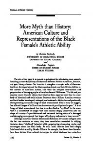
ary colors) is made up by the following cases: (B1) Spectral (i.e. monochromatic) lights and purple lights (additive mixtures of two spectral lights from the violet and the red ‘end’ of the spectrum, respectively) whose chromaticity makes up the outer boundary of the well-known C.I.E. chromaticity diagram (see e.g. Wyscecki and Stiles, 1982). These lights correspond to the maximally saturated (and hence pronouncedly chromatic) α-colors across the entire hue circle. (B2) At the ‘bottom’ the light a = 0 that evokes intrinsic gray. (B3) At the ‘upper end’, extremely bright-looking lights of luminance Lmax . We are now ready to state the announced empirical Observation, which, while being clearly weaker than Observation 1, is is still sufficiently strong to derive the central dimensionality result of Section 4. Observation 2 There are interior lights a1 and factors t1 , 0 ≤ t1 < 1, such that the following holds: (C1) (t1 ∗ a1 , a1 ) 6∼ (c, c) for all lights c; (C2) (t ∗ a1 , a1 ) 6∼ (b, b) for all factors t, t1 < t < 1, and all boundary lights b. That is, given some such light a1 and factor t1 , we are interested in the stimuli (t ∗ a1 , a1 ) and the resulting ‘continuous path’ of focal colors as t is varied between t1 and 1 (compare figure 3). The strict criterion (5) of Observation 1 is only required to hold for t = t1 here, i.e. only the focal color evoked by (t1 ∗ a1 , a1 ) is postulated to be a β-color (C1) (so, in particular, Observation 0 trivially pops out). For the other stimuli (t ∗ a1 , a1 ) it is only required that the focal colors evoked are no boundary colors (C2). The validity of this observation can easily be demonstrated by considering, for example, a white light a1 of a luminance that is clearly smaller than Lmax but sufficiently high so that the l.i.p. (a1 , a1 ) evokes a ‘nice’ bright white. For the factor t1 we may, for instance, choose the value .4. Then the stimulus (t1 ∗ a1 , a1 ) will clearly evoke a β-color, namely, a ‘nice’ gray (which does not look dim as i.p.’s or l.i.p.’s of very low luminance or intrinsic gray). 21

Figure 3: An illustration of the path considerd as an example for Observation 2. Left column: schematic representation of the stimuli; middle column: intensity profiles of these stimuli; right column: schematic representation of what they look like. The right column cannot convey a fully appropriate impression of the colors evoked in a completely dark outer surround, however.

22

So, C1 is satisfied. And the stimuli (t ∗ a1 , a1 ) will evoke lighter and lighter shades of gray and eventually white as t is varied from t = t1 to 1. So they are clearly different from the boundary colors of all three categories B1, B2, and B3. Hence condition C2 is also satisfied. Many other examples could be found. Moderately saturated chromatic lights a1 , for instance, would do the job just as well. A final remark: As promised before, Observation 0, 1, and 2 indeed only refer to color matching, postulating certain mismatches. In this connection it is important to note that the lights a1 and factors t1 in Observation 2 can be chosen in such a way that the mismatches postulated in C1 and C2 are very pronounced mismatches. Furthermore each of these mismatches involves a clear difference in some quality which even in traditional accounts would count as an attribute of ‘color proper’, such as brightness, the differences among various shaded of gray and white, or the distinction between chromatic and achromatic colors. So even from a more traditional perspective, these considerations cannot easily be dismissed as referring to some perceptual attribute external to ‘color’.

4

Dimensionality Theorems

Here, finally, are the announced dimensionality theorems. The core theorems in section 4.1 solely build on the Observations (with capital ‘O’) as discussed in the previous section. This is done here so as to a achieve a maximal degree of rigour and transparency in the corresponding arguments and to free them from any unnecessary conceptual and empirical burden. Some readers may perhaps prefer to get a more qualitative understanding of what is going on here, say, in terms of color attributes, which deliberately are excluded from consideration in section 4.1. They are invited to read this section in conjunction with the corresponding examples and qualititative descriptions provided in the previous section; further qualitative considerations that could be helpful in this connection are also found later on.

23

4.1

Central Theorems and Proof

Dimensionality Theorem 1 Assume that Observation 1 holds along with extended trichromacy, and let h be an N -dimensional continuous focal color code (for center-surround stimuli) w.r.t. some primary color code φ. Then N ≥ 4. Dimensionality Theorem 2 Assume that Observation 2 holds along with extended trichromacy, and let h be an N -dimensional continuous focal color code (for center-surround stimuli) w.r.t. some primary color code φ. Then N ≥ 4. Proofs. If Observation 1 is satisfied, then so is Observation 2. So Theorem 1 follows from Theorem 2.16 So let us directly turn to Theorem 2. In this paper, I will only sketch a somewhat simplified version of the proof that conveys the key idea, though. A two-dimensional illustration of the three-dimensional situation considered in the proof is given in figure 4. The proof is based on an indirect argument, i.e., a reductio ad absurdum. To this end, we will assume that Observation 2 holds and that, contrary to the above claim, there were a three-dimensional continuous focal color code h w.r.t. φ. A contradiction will be derived. To keep the argument elementary, we will (with no loss of generality) make the simplifying additional assumption that for all lights a, the code h satisfies h[φ(a), φ(a)] = φ(a).

(6)

This may be considered a natural special case anyway, since equation (6) already defines a ‘partial’ three-dimensional continuous focal color code for l.i.p.’s (a, a) (due to extended trichromacy). The assumption considered here then means that this partial code can be extended three-dimensionally to the entire gamut of center-surround stimuli.17 Now, choose some light a1 and factor t1 according to Observation 2. Let us focus attention on the stimuli 16

For an instructive proof of Theorem 1 that directly exploits the strong postulates of Observation 1, see Niederée (1998, sec. 6.2). 17 Mathematical remark: Of course, all that matters for the general case is whether this special case may really be considered “with no loss of generality”. In fact, for the general case one needs to invoke a well-known and deep topological theorem, the so-called gamut invariance theorem. This allows one to establish, first of all, that because of extended trichromacy an N -dimensional continuous focal color code must satisfy N ≥ 3 (i.e., the possibility N = 1 or 2 can indeed be ruled out). Now let us assume that h is a three-

24

Figure 4: Two-dimensional illustration to the proof of Dimensionality Theorem 2 (see text). To render this illustration three-dimensional just embed the whole situation into three-dimensional space while replacing the triangle with the truncated cone shown in figure 2; the outer surfaces of that cone then jointly constitute the boundary ∂C ∗ .

25

(t∗a1 , a1 ) (t ≤ 1) and consider the h-codes assigned to these stimuli. These are the vectors ht := h[φ(t∗a1 ), φ(a1 )],

0 < t ≤ 1.

(7)

Because h is assumed to be continuous, the function that assigns the vector ht to t is a continuous function defining a continuous path in Re3 . Now, condition C1 of Observation 2 along with condition (3) of the definition of a focal color code, imply that ht1 = h[φ(t1 ∗ a1 ), φ(a1 )] differs from the codes h[φ(a), φ(a)] for all vectors φ(a) ∈ C ∗ . Because of (6), this simply means that ht1 lies outside of C ∗ (point e in figure 4). In contrast, h1 , which because of equation (6) is simply the code φ(a1 ), belongs to the interior of C ∗ (point i in figure 4). Hence, the continuous path ht , t1 ≤ t ≤ 1, connects the interior and the exterior of C ∗ . In consequence, this path must somewhere intersect the boundary ∂C ∗ of C ∗ . In other words, for some boundary light b and some real number t2 , t1 < t2 < 1, we must have that φ(b) = ht2 . Because of (6) and the definition of ht given in (7), this implies that h[φ(b), φ(b)] = h [φ(t2 ∗a1 ), φ(a1 )] . Hence, by (3), (b, b) ∼ (t2 ∗ a1 , a1 ), contradicting the choice of a1 and t1 (condition C2 of Observation 2). This is the announced contradiction showing that the assumption N = 3 is not compatible with Observation 2, and hence N ≥ 4 follows. This completes the proof. dimensional continuous focal color code. Observing that, by assumption, the function h′ (φ(a)) := h[φ(a), φ(a)] is continuous and one-to-one, and that C ∗ is a compact subset of Re3 , the gamut invariance theorem (plus some standard continuity-based arguments) allows one to establish that h′ [C ∗ ] is again a compact subset of Re3 , the boundary and interior of C ∗ being mapped into the boundary and interior of h′ [C ∗ ], respectively. Having established this, the proof sketched in this paper (based on the additional assumption that h′ is the identity function) can be easily transferred to the general case. To do so, in certain places of the argument presented here (including the illustration), C ∗ has to be replaced with the set h′ [C ∗ ] and ∂C ∗ with its boundary. For a close variant of this theorem, the complete general proof is given in Niederée (1998, section 6, see in particular sections 6.1 and 6.4.2). Note that the argument presented hereafter mathematically also relies on the compactness of h′ [C ∗ ] along with the consideration of a suitable infimum or supremum.

26

Note that for N ≥ 4, the problem encountered in the proof for N = 3 disappears because, thanks to the additional dimension(s), the corresponding path ht can then simply bypass ∂C ∗ . This is analogous to the two-dimensional situation of a square in a plane. Every continuous path in the plane connecting a point i in the interior of the square with a point e outside the square must pass through the boundary of the square. But when embedded into a three-dimensional situation, the path could easily bypass that boundary.

4.2

Further examples of the method

The above dimensionality theorems are just examples of a general method. Many variants of these theorems are in fact possible where the above definition of a continuous focal color code mutatis mutandis is applied to other classes of stimuli and associated ‘color spaces’. May it suffice here to briefly mention two examples. The first example concerns focal colors evoked by achromatic centersurround stimuli (t ∗ w, w) (t ≥ 0). Proponents of the mainstream view would postulate that there is a one-dimensional continuous focal color code (‘brightness’) for those stimuli. By the above method it can easily be shown that such a code has to be at least two-dimensional. In fact, all of the relevant empirical observations have already been mentioned. Here is an informal and somewhat sloppy sketch of the argument (where stimuli, evoked focal colors and the associated color codes are simply lumped together). This sketch can easily be made precise along the lines of Observation 2 and Dimensionality Theorem 2, however. To begin with, consider a bounded one-dimensional space of achromatic α-colors evoked by l.i.p stimuli involving achromatic lights with a luminance ≤ Lmax (evoking white of varying brightness). The boundary here simply consists of the two ‘endpoints’: intrinsic gray (no light) and a very bright white evoked by an achromatic light of luminance Lmax . As discussed before, there exists a continuous path of achromatic colors evoked by stimuli (t∗w, w) (t1 ≤ t ≤ 1) that connects the interior of this bounded one-dimensional space with a ‘nice’ gray outside of this space. As can be observed empirically, this path does not pass through the two just-mentioned ‘endpoints’ serving here as our boundary colors. So the extended achromatic color space must be more than one-dimensional. The second example concerns a potential application of the above method. A closer inspection of the above observations and arguments reveals that only 27

stimuli of the form (t∗a, a),

for t ≤ 1,

are actually referred to, i.e., homochromatic decrements and l.i.p.’s, which jointly will be called weak homochromatic decrements. This means that the above Dimensionality Theorems remain true if the phrase “for centersurround displays” is replaced by “for weak homochromatic decrements”. Having established this, one might in fact go one step further and propose the hypothesis that for these stimuli a full-fledged four-dimensional account is appropriate, meaning that both φ(a) and the factor t are assumed to make an independent contribution to the evoked color. Observation 1 would be a simple consequence of this hypothesis. Mathematically speaking, this means the corresponding color space makes up a four-dimensional manifold (in which the achromatic colors constitute a two-dimensional submanifold). This is not yet implied by the above Dimensionality Theorems themselves (see next section). But it seems quite plausible with regard to the phenomenon of blackishness induction discussed in section 3. So, for the sake of argument, assume there is indeed a four-dimensional continuous focal color code of that kind for weak decrements. If we now extend the scope again to arbitrary center-surround stimuli (a, b), the question arises whether for these stimuli four dimensions will do, or whether a more than four-dimensional continuous focal color code is needed. In principle, at least, one could then try to show the latter by applying the above method again, that is, by looking for ‘new colors’ (relative to these stimuli/colors) and by studying suitable continuous paths connecting these new colors and the ones evoked by weakly homochromatic decrements, the crucial boundary now being itself three-dimensional. If some such path could be shown not to pass through this boundery, the desired conclusion would follow. Such ‘new’ colors seem to exist indeed, such as, for instance focal colors that may be described as simultaneously reddish and greenish, or as bluish and yellowish (see e.g. Ekroll, Faul, Niederée, and Richter, 2002), as well as, it appears to me, certain shades of brown. But all this is certainly an open issue, which in particular concerns the question as to whether a corresponding counterpart to Observation 2 can be established empirically. Certainly the corresponding relevant mismatches will be more subtle than those involved in our dicussion of Observation 2. The same goes all the more for the question whether or not dimensionality (in the present sense) goes up even further if more complex displays are considered. 28

5

Discussion

Now, what do the above results tell us above and beyond what has been said so far? This question will be approached from two perspectives. First, we will raise the question as to how the above type of result is related to various concepts of dimensionality. In section 5.1 this is briefly discussed from a sensation-oriented perspective. Second, we will be concerned with the question of what such results could mean for our understanding of color perception in general. This necessitates a more careful juxtaposition of what has been called here a sensation- and a perception-oriented approach. These matters will be discussed in the concluding section 5.2 (which can be read independently of the following discussion of dimensionality concepts).

5.1

Dimensions of Dimensionality

Our discussion of the first issue will take into account both the intrinsic aspects mentioned in section 2.3 and the extrinsic ones. Let us begin with the latter. The above theorems simply tell us that all standard three-dimensional models of asymmetric color matching that purport to refer to perfect focal matches, are fundamentally flawed empirically, and the same goes for onedimensional models in the achromatic case. That is, all of these models— provided they are indeed continuous and in line with criterion (3)—will be inconsistent with the premises of the theorems. As for Dimensionality Theorem 2, this means that any such model must be at odds with extended trichromacy or with Observation 2 (or both). The former is the case, for instance, for a ratio-based model as specified by equation (4), for this implies that the same code is assigned to arbitrary l.i.p.’s (a, a) and (b, b), viz. the code (1, 1, 1). By criterion (3) this would imply that these stimuli should look the same. On the other hand, if a model is at odds with Observation 2, this means that for some lights a1 and factors t1 which satisfy conditions C1 and C2, the model implies a match where C1 or C2 postulate a mismatch. Since a1 and t1 can be chosen in such a way that these mismatches are pretty pronounced ones, this can hardly be counted as a tolerable failure of such a model. The intrinsic aspects mentioned in section 2.3 concern the topology of color space, or more precisely, of color spaces, proceeding step by step from more restricted color spaces (associated with certain classes of stimuli) to possibly more comprehensive ones as illustrated above. Results like Dimen29

sionality Theorem 2 are but a first step in such a project, and only a few, more or less intuitive, remarks along these lines can be made here. For brevity’s sake, we will continue focusing attention to colors evoked by center-surround displays (in dark outer surround) unless stated otherwise. The following account easily generalizes to other situations, however. Let N0 denote the least number N for which there is an N -dimensional continuous focal color code (for center-surround stimuli). From a topological viewpoint, this number may be termed the global dimensionality (in the sense of an embedding into ReN ) of the space of focal colors evoked by centersurround stimuli. The above Dimensionalty Theorems then state that this global dimensionality is at least four. Now, by way of comparison, consider the following figures (conceived as topological spaces of points), which are globally two-dimensional in this sense: (i) a circle, understood as a closed line; (ii) a cross in the sense of two lines intersecting at a point P ; and (iii), a filled circle (including the enclosed area). In example (i), the situation is locally only one-dimensional everywhere. In case (ii), we may speak of a locally ‘> 1-dimensional’ situation at P , while in case (iii) the situation is not only > 1-dimensional everywhere, but in fact locally properly two-dimensional, constituting a two-dimensional manifold. Analogously, the conclusion N ≥ 4 of the above dimensionality theorems does not by itself rule out the possibility illustrated by case (i): Locally, the space of focal center-surround colors could perhaps still be three-dimensional everywhere. However, a closer inspection of the situation considered in the proof of the theorem shows that this possibility can indeed be ruled out.18 Having established this, one might then venture the hypothesis that for the focal colors evoked by center-surround displays, the situation is in fact analogous to case (iii), be it for N = 4, 5, or perhaps even 6 (with possibly a few special regions which call for a separate treatment). Recall that for the color space associated with weak decrements only, a corresponding hypothesis that postulated local four-dimensionality has been proposed in section 4.2. Strong dimensionality hypotheses of that kind can be sustained by the method discussed before, but they cannot be inferred this way directly. This will always constitute an additional, though often plausible, theoretical step. 18

It can be shown that along the path ht considered in the proof of Theorem 2 there must be a point p where the situation becomes locally > 3-dimensional. If Observation 1 is assumed to hold, this is already occurs at the very beginning of this path (p = i). For mathematical details and further consideration along these lines see Niederée (1998, section 6.5.4).

30

One noteworthy consequence of these considerations is that the possibility of obtaining (perfect) asymmetric color matches is far more restricted than often assumed in standard asymmetric color matching paradigms. For instance, in such an experiment, a subject may be asked to find a light a′ such that—for lights a, b, and b′ fixed by the experimenter—a (perfect) focal match obtains between the center-surround stimuli (a, b) and (a′ , b′ ) (with a dark outer surround). This will often be impossible, even if b and b′ are rather similar. Problems of that kind have in fact been reported in various studies for various types of stimuli (see e.g. Logvinenko & Maloney, 2006, to mention just one recent example). This observation is usually neglected, however, in the mainstream literature. In a way, one problem of standard three-dimensional models of asymmetric color matching is in fact that they imply too many matches. So far we have pointed out that a statement concerning ‘the dimensionality of color space’ needs to specify the range of colors considered as well as features such as whether the concept is understood locally or globally. Even more conceptual ‘dimensions’ of the concept of dimensionality need to be taken into account that play a role in the color literature. So far, we have focused on a concept of output dimensionality that is essentially topological in nature. Dimensionality concepts could also be based on different criteria, giving rise to different concepts of dimensionality (none of which is the ‘true’ one; they just capture different, though related, aspects of the situation). One could for instance ask for the least number M for which there is a focal color code h = (h1 , . . . , hM ) satisfying criterion (3) such that one of the following criteria is fulfilled: • Each component code hi is a (univariant) neural code capturing neural activity at some level of color processing. • The component codes hi are associated with perceptual attributes. • The code h represents subjective proximity judgments by some metric on ReM in the sense of a suitable concept of multidimensional scaling (mds; see e.g. Suppes et al., 1989, Chapter 14). Usually this will mean that some such criterion is imposed in addition to that of continuity, the latter often being assumed tacitly. Provided there is a corresponding code at all, the minimal number M fulfilling such an additional criterion (i.e. the corresponding ‘dimensionality’) will of course satisfy the 31

inequality M ≥ N0 (and hence in the present situation, M ≥ 4). Conversely, if for a class of stimuli, evidence is provided for M ≥ k (for some integer k), this does not automatically imply that the corresponding topological global dimensionality N0 also satisfies this inequality because possibly M > N0 This observation is relevant, in particular, to mds-based criteria, which are quite popular in the color (and brightness) literature.19 That the mds-based dimensionality may easily exceed topological dimensionality is illustrated by the following example: A U-shaped line in a plane is onedimensional from a topological point of view (both globally and locally), but in order to represent the distances within this line by a Euclidean metric, say, two dimensions are required. My impression is that this observation applies to various mds-based studies that, for certain classes of stimuli, suggest a ‘higher dimensional’ approach to color or ‘brightness’ (i.e. M ≥ 4 or M ≥ 2, respectively). However, there are exceptions, which also suggest higher dimensionality at a topological level. In a recent mds-based study, for instance, Logvinenko and Maloney (2006) investigated focal colors in achromatic stimuli (though in a somewhat different setting than the one considered here). They reach the conclusion that in their setting achromatic colors make up a two-dimensional manifold (implying N0 = 2 for the corresponding color space).

5.2

Color sensation vs. color perception reconsidered

In their study, Logvinenko and Maloney actually employed stimuli that consisted of central fields of varying surface reflectance embedded into a variegated surround, both of which were exposed to a homogeneous illumination of varying intensity (luminance). According to their two-dimensional model, both the surface reflectance and the intensity of the illumination make an independent contribution to the proximity judgments made by the subjects. This leads us back to issues concerning color perception and to issues relating to perceived surface color and approximate color constancy. Restricting attention to matte surfaces, perceived surface color, too, is usually discussed in terms of three dimensions (color solids). Correspondingly, achromatic surface colors are accounted for in terms of one dimension 19

Note that the inequality M ≥ N0 here only holds for the ‘true’ dimensionality w.r.t. the respective mds model (provided the model is satisfied at all for the situation considered). The estimated dimensionality reported in such studies, based on empirical judgments and models that allow for the possibility of judgmental errors, may sometimes be smaller.

32

(albedo or lightness, ranging qualitatively from black via different shades of gray to white). This trivariance of surface color (referring to the perceptual ‘output’ in complex scenes, i.e. to perceived surface colors) needs to be carefully distinguished from trichromacy as discussed in section 2 above. It is not fundamentally called into question by our approach either; but it needs to be carefully qualified. For, if the illumination in a physical scene is changed, then the overall appearance of the surfaces will typically change even if the involved perceived surface colors themselves remain (more of less) constant in the sense of color constancy. This difference may be attributed to a difference in the perceived ‘illumination color(s)’, which is as much a component of the percept as are the perceived surface colors themselves. On this view, the visual system decomposes the locally three-dimensional input into two trivariant components (layers, scissions) for each direction in the visual field (color segmentation). And the situation further complicates, if (perceived) transparency, gloss, self-luminosity of objects etc. are taken into account, i.e., what Katz (1911/1935) termed ‘modes of color appearance’ (‘Erscheinungsweisen der Farben’ ). Similar points have already been made in the early color literature, e.g. by Katz (1911/1935), Hering (1920), Bühler (1922), and Gelb (1929), and have been repeatedly brought up again by later authors; see e.g. Adelson (1993), Arend (1994) and other papers in Gilchrist (1994), Ekroll et al. (2002; cf. MacLeod, 2003), Mausfeld (1998, 2003)). Nevertheless, many accounts of color vision ignore these complexities to the present day. From this perspective, the above results do in fact not come as much of a surprise. However, I do not think that sensation-oriented aspects of color vision discussed above simply reduce to these complexities of color perception proper. It seems, in fact, that both a sensation-oriented and a perceptionoriented aspect (‘level’, ‘mode’) coexist in the phenomenology of color vision itself, at least to some extent and in a subtly interwoven manner. First, there is the level of a field of colors, which are not ‘yet’ attached to perceived objects in perceptual space or perceived illumination (for short: field colors). And, secondly, at the object-centered level we get surface colors, transparent layer colors, illumination colors etc. (for short: segmented colors). The latter may sometimes be more or less ‘vague’, though. This is particularly true of the reduced stimuli considered in the previous sections, where one might at best speak of an “embryonic” form of segmentation (Mausfeld, & Niederée, 1993). These phenomenal levels do not kick around independently of each other, of course. Instead, there is some kind of phenomenal binding connecting them. 33

To put it very simply, in each direction of visual space a field color appears to be associated with the corresponding bundle of segmented colors. Consider, for example, the case where a yellow transparent layer appears to cover part of a blue or red surface, respectively (segmented colors); at the location of the overlapping region we then often simultaneously see a green or orange, respectively (field colors). This distinction may also help to settle debates as that between Hering (e.g. 1920, p. 210) and von Kries (in Helmholtz, 1910, pp. 490 ff.). They had a dispute about the question whether a gray patch on a wall (in terms of perceived surface colors) should be counted as the same sensation (Empfindung) as a suitable gray-looking shadow on a white wall, as advanced by von Kries, or not, as claimed by Hering. Von Kries’ position may possibly be adequate for the field level, while Hering clearly refers to the segmented level. The two levels distinguished here are closely related to the concept of a double representation of color in Arend (1994, see also Arend and Reeves, 1986), who juxtaposed unasserted and attributed colors in a similar manner (see also, in a philosophical context, Cohen, in press). In similar vein, Evans (1974, ch. 11) already pointed out not only that in color vision there is both an “object frame of reference” and an “illumination frame of reference” (which corresponds to our notion of ‘segmented colors’), but also that in addition there is a “stimulus frame of reference”. In this connection he explicitly warned against an “either-or-fallacy” (p. 193). Sometimes, an analogous duality of perception is also invoked in discussions of perception in general (including e.g. the perception of size and shape). Examples are Helmholtz’s distinction of a ‘Sehfeld’ (visual field) and a ‘Sehraum’ (visual space), or Gibson’s (1950) distinction between a ‘proximal mode’ and a ‘world mode’ (see also Rock, 1983, and Todorović, 2002). And the picture gets even more complex if one takes into account duality phenomena at the segmented level as involved, e.g., in picture perception (see e.g. Heyer & Niederée, 2003). If one accepts the basic distinction just made, then it is clear that the just-mentioned complexities at the level of segmentated colors do not by themselves imply a corresponding degree of complexity (or ‘dimensionality’) at the level of field colors. It seems that a specific field color (e.g. a certain orange) may in fact be phenomenally associated with different segmentations (such as a yellow transparent layer in front of a red one; or simply an orange surface appearing in neutral illumination, and so forth). This in particular means that color segmentation is not per se inconsistent with a three-dimensional account of field colors. In fact, authors entertaining some 34

such distinction of levels or modes often assume three-dimensionality to hold for what is called here the level of field colors. However, by the above dimensionality results (or related findings reported in the literature, such as, in my view at least, Logvinenko & Maloney, 2006) this possibility is ruled out, however. For these results obviously refer to field colors, thus impliying that a higher dimensional approach is already needed to provide an appropriate account for this seemingly ‘basic’ level of color vision.20 So they provide us with an additional piece of information about color vision, indeed. As a consequence, the level of field colors should not simply be conceived as a ‘proximal mode’ of color vision. It rather seems to foreshadow some of the complexities showing up at the segmented level, though in a much more rudimentary fashion. And this might in turn play a role in the management of perceptual ambiguity by ‘representing’ certain possible ambiguities in the precept itself. In my view, a standard representational or realist account of color vision (among other things) cannot account for the existence of the field level and its relation to the segmented level. Nor can it straightforwardly incorporate simple everyday observations such as the fact that intrinsic color qualities such as, say, appearing greenish or brownish may pertain both to the field level and to the segmented level, and here in turn to colors that are perceived as belonging to surfaces, transparent layers, or (in the case of greenish at least) to self-luminous objects or illumination. For, what should all these cases have in common in the represented outer world? These are but elementary examples of a rich internal structure governing human color vision, still waiting to be described systematically. Continuous path analysis, i.e. investigations into the effect of gradual stimulus variations (which may result in gradual or disrupt changes at the perceptual level, as the case may be) may be expected to yield important insights in this connection also way beyond the issue of dimensionality. And the same, I believe, goes for accounts of various types of dimensionality, provided they are subsumed under the more general goal of understanding the intricate internal overall logic underlying 20

As pointed out, this already holds for the focal colors in center-surround displays. But the method of continuous path analysis can be brought to bear just as well on other classes of stimuli and the field colors they evoke, yielding higher dimensionality, e.g., for the field colors going together with surfaces viewed under different illuminations, or with certain gradual transitions between different modes of color appearance at the segmented level, such as (perceived) self-luminous vs. surface colors. See e.g. Niederée, 1998, Sect. 6.5 and 7.

35

human color vision.

References Adelson, E. H. (1993). Perceptual organization and the judgment of brightness. Science, 262, 2042–2044. Arend, L. E. (1994). Surface colors, illumination, and surface geometry: Intrinsic-image models of human color perception. In A. L. Gilchrist (Ed.), Lightness, Brightness, and Transparancy (pp. 159–213). Hillsdale: Erlbaum. Arend, L. E., & Reeves, A. (1986). Simultaneous color constancy. Journal of the Optical Society of America A, 3 , 1743–1751. Brindley, G. S. (1960). Physiology of the Retina and the Visual Pathway. London: Arnold. Bühler, K. (1922). Die Erscheinungsweisen der Farben. In K. Bühler (Ed.), Handbuch der Psychologie. I. Teil. Die Struktur der Wahrnehmungen (pp. 1–201). Jena: Fischer. Cohen, J. (in press). Color constancy as counterfactuals. Australasian Journal of Philosophy. Ekroll, V., Faul, F., Niederée, R., & Richter, E. (2002). The natural center of chromaticity space is not always achromatic: A new look at color induction. Proceedings of the National Academy of Sciences U.S.A., 99 (20), 13352– 13356. Evans, R.M. (1974). The Perception of Color . New York: Wiley. Gelb, A. (1929). Die ‘Farbenkonstanz’ der Sehdinge. In A. Bethe, G. v. Bergmann, G.Embden, & A. Ellinger (Eds.), Handbuch der normalen und pathologischen Physiologie. Bd. 12, 1. Hälfte. Receptionsorgane II. (pp. 594– 678). Berlin: Springer. Gibson, J. J. (1950). The Perception of the Visual World. Boston: Mifflin. 36

Gilchrist, A. L. (Ed.) (1994). Lightness, Brightness, and Transparency. Hillsdale: Earlbaum. Grassmann, H. (1853). Zur Theorie der Farbmischung. Poggendorff ’s Annalen der Physik, 89 69–84. Grassmann, H. (1854). On the theory of compound colours. Philosophical Magazine, Series 4, 7 , 254–264. Heggelund, P. (1974). Achromatic color vision. I. Perceptive variables of achromatic colors. Vision Research, 14 , 1071–1079. Helmholtz, H. von (1910). Handbuch der Physiologischen Optik, Bd. 3. (3rd edition, edited by A. Gullstrand, J. v. Kries & W. Nagel). Hamburg: Voss. Hering, E. (1920). Grundzüge der Lehre vom Lichtsinn. Berlin: Springer. Katz, D. (1911). Die Erscheinungsweisen der Farben und ihre Beeinflussung durch die Individuelle Erfahrung. Leipzig: Barth. (English Translation: The World of Color , translated from the 2nd German edition by R.B. MacLeod and C.W. Fox, London, 1935.) Krantz, D. H. (1975). Color measurement and color theory. I. Representation theorem for Grassmann structures. Journal of Mathematical Psychology, 12 , 183–303. Krantz, D.H. & Simon, C.P. (1983) The topological laws of color matching. Unpublished manuscript. Logvinenko, A. D., & Maloney, L. T. (2006). The proximity structure of achromatic surface colors and the impossibility of obtaining asymmetric lightness matching. Perception and Psychophysics, 68, 76–83. MacLeod, D. I. A. (1986). Receptoral constraints on colour appearance. In D. Ottoson & S. Zeki (Eds.), Central and Peripheral Mechanisms of Colour Vision (pp. 66–81). London: Macmillan. MacLeod, D. I. A. (2003). New dimensions in color perception. Trends in Cognitive Science, 7 (3), 97–99. 37

Mausfeld, R. (1998). Color perception: From Grassmann codes to a dual code for object and illumination colors. In W. G. K. Backhaus, R. Kliegl, & J. S. Werner (Eds.), Color Vision (pp. 219–250). Mausfeld, R. (2003). ‘Colour’ as part of the format of different perceptual primitives: The dual coding of color. In R. Mausfeld, & D. Heyer (Eds.), Colour Perception. Mind and the Physical World (pp. 381–429). Oxford: Oxford University Press. Mausfeld, R., & Niederée, R. (1993). An inquiry into relational concepts of colour based on incremental principles of colour coding for minimal relational stimuli. Perception, 22, 427–462. Niederée, R. (1998). Die Erscheinungsweisen der Farben und ihre stetigen Übergangsformen. Post-doctoral Thesis (Habilitation), Philosophische Fakultät der Christian-Albrechts-Universität zu Kiel, Kiel. Niederée, R., & Heyer, D. (2003). The dual nature of picture perception: A challenge to current accounts of visual perception. In H. Hecht, R. Schwartz, & M. Atherton (Eds.), Looking into pictures (pp. 77–98). Cambridge/Mass.: MIT Press/Bradford books. Niederée, R., & Mausfeld, R. (1997). Increment-decrement asymmetry in dichoptic matching with haploscopically superimposed displays. Vision Research, 37, 613–615. Rock, I. (1983). The Logic of Perception. Press/Bradford Books.

Cambrigde/MA: MIT

Suppes, P., Krantz, D. H., Luce, R. D., & Tversky, A. (1989). Foundations of Measurement. Vol. II. Geometrical, Threshold, and Probabilistic Representations. San Diego: Academic Press. Todorović, D. (2002). Comparative overview of perception of distal and proximal visual attributes. In D. Heyer & R. Mausfeld (Eds.), Perception and the Physical World (pp. 37–74) Whittle, P. (2003). Contrast colours. In R. Mausfeld, & D. Heyer (Eds.), Colour Perception. Mind and the Physical World (pp. 115–138). Oxford: Oxford University Press. 38

Whittle, P., & Challands, P. D. C. (1969). The effect of background luminance on the brightness of flashes. Vision Research, 9 , 1095–1110. Wyszecky, G., & Stiles, W. S. (1982). Color Science. Concepts and Methods, Quantitative Data and Formulae. (2nd edition) New York: Wiley.

39