Morphological operation-based bi-dimensional empirical mode decomposition for automatic background removal of fringe patterns Xiang Zhou,1,2,* Adrian Gh. Podoleanu, 2 Zhuangqun Yang,3 Tao Yang,1 and Hong Zhao1 1
State Key Laboratory Manufacturing Systems Engineering, Xi’an Jiaotong University, Xi’an, Shaanxi, 710049, China 2 School of Physical Sciences, University of Kent, Canterbury, CT2 7NH, UK 3 The First Affiliated Hospital of Medical College of Xi'an Jiaotong University, Xi’an, Shaanxi, 710061, China *
[email protected]
Abstract: A modified bi-dimensional empirical mode decomposition (BEMD) method is proposed for sparsely decomposing a fringe pattern into two components, namely, a single intrinsic mode function (IMF) and a residue. The main idea of this method is a modified sifting process which employs morphological operations to detect ridges and troughs of the fringes, and uses weighted moving average algorithm to estimate envelopes of the IMF, replacing respective local extrema detection and envelope interpolation of conventional BEMDs. The background intensity of the fringe pattern is automatically removed by extracting the single IMF, thereby relieving the mode mixing problem of the BEMDs. A fast algorithm based on 2D convolution is also presented for reducing the calculation time to several seconds only. This approach is applied to process simulated and real fringe patterns, and the results obtained are compared with Fourier transform, discrete wavelet transform, and other EMD methods. The MATLAB code is downloadable at http://gr.xjtu.edu.cn/web/zhouxiang. ©2012 Optical Society of America OCIS codes: (100.2650) Fringe analysis; (110.2650) Fringe analysis; (120.2650) Fringe analysis.
References and links 1. 2. 3. 4. 5. 6. 7. 8. 9. 10. 11. 12. 13.
M. Servin, J. L. Marroquin, and F. J. Cuevas, “Demodulation of a single interferogram by use of a twodimensional regularized phase-tracking technique,” Appl. Opt. 36(19), 4540–4548 (1997). M. Takeda and K. Mutoh, “Fourier transform profilometry for the automatic measurement of 3-D object shapes,” Appl. Opt. 22(24), 3977–3982 (1983). J. A. Quiroga, J. Antonio Gómez-Pedrero, and Á. García-Botella, “Algorithm for fringe pattern normalization,” Opt. Commun. 197(1-3), 43–51 (2001). X. Su and W. Chen, “Reliability-guided phase unwrapping algorithm: a review,” Opt. Lasers Eng. 42(3), 245– 261 (2004). Q. Kemao, “Windowed Fourier transform for fringe pattern analysis,” Appl. Opt. 43(13), 2695–2702 (2004). J. Zhong and J. Weng, “Dilating Gabor transform for the fringe analysis of 3-D shape measurement,” Opt. Eng. 43(4), 895 (2004). J. G. Zhong and J. W. Weng, “Spatial carrier-fringe pattern analysis by means of wavelet transform: wavelet transform profilometry,” Appl. Opt. 43(26), 4993–4998 (2004). L. R. Watkins, S. M. Tan, and T. H. Barnes, “Determination of interferometer phase distributions by use of wavelets,” Opt. Lett. 24(13), 905–907 (1999). J. G. Zhong and J. W. Weng, “Phase retrieval of optical fringe patterns from the ridge of a wavelet transform,” Opt. Lett. 30(19), 2560–2562 (2005). M. A. Gdeisat, D. R. Burton, and M. J. Lalor, “Eliminating the zero spectrum in Fourier transform profilometry using a two-dimensional continuous wavelet transform,” Opt. Commun. 266(2), 482–489 (2006). A. Federico and G. H. Kaufmann, “Phase retrieval in digital speckle pattern interferometry by use of a smoothed space-frequency distribution,” Appl. Opt. 42(35), 7066–7071 (2003). S. Ozder, O. Kocahan, E. Coşkun, and H. Göktaş, “Optical phase distribution evaluation by using an Stransform,” Opt. Lett. 32(6), 591–593 (2007). J. G. Zhong and J. W. Weng, “Generalized Fourier analysis for phase retrieval of fringe pattern,” Opt. Express 18(26), 26806–26820 (2010).
#172970 - $15.00 USD (C) 2012 OSA
Received 20 Jul 2012; revised 27 Aug 2012; accepted 9 Sep 2012; published 8 Oct 2012 22 October 2012 / Vol. 20, No. 22 / OPTICS EXPRESS 24247
14. Q. Kemao, “On window size selection in the windowed Fourier ridges algorithm,” Opt. Lasers Eng. 45(12), 1186–1192 (2007). 15. N. E. Huang, Z. Shen, S. R. Long, M. L. C. Wu, H. H. Shih, Q. N. Zheng, N. C. Yen, C. C. Tung, and H. H. Liu, “The empirical mode decomposition and the Hilbert spectrum for nonlinear and non-stationary time series analysis,” Proc. R. Soc. London Ser. A-Math. Phys. Eng. Sci. 454(1971), 903–995 (1998). 16. M. B. Bernini, G. E. Galizzi, A. Federico, and G. H. Kaufmann, “Evaluation of the 1D empirical mode decomposition method to smooth digital speckle pattern interferometry fringes,” Opt. Lasers Eng. 45(6), 723– 729 (2007). 17. S. Li, X. Su, W. Chen, and L. Xiang, “Eliminating the zero spectrum in Fourier transform profilometry using empirical mode decomposition,” J. Opt. Soc. Am. A 26(5), 1195–1201 (2009). 18. M. B. Bernini, A. Federico, and G. H. Kaufmann, “Noise reduction in digital speckle pattern interferometry using bidimensional empirical mode decomposition,” Appl. Opt. 47(14), 2592–2598 (2008). 19. M. Wielgus and K. Patorski, “Evaluation of amplitude encoded fringe patterns using the bidimensional empirical mode decomposition and the 2D Hilbert transform generalizations,” Appl. Opt. 50(28), 5513–5523 (2011). 20. X. Zhou, H. Zhao, and T. Jiang, “Adaptive analysis of optical fringe patterns using ensemble empirical mode decomposition algorithm,” Opt. Lett. 34(13), 2033–2035 (2009). 21. S. M. A. Bhuiyan, N. Attoh-Okine, K. E. Barner, A. Y. Ayenu-Prah, and R. R. Adhami, “Bidimensional empirical mode decomposition using various interpolation techniques,” Adv. Adapt. Data Anal 01(02), 309–338 (2009). 22. X. Zhou, T. Yang, H. Zou, and H. Zhao, “Multivariate empirical mode decomposition approach for adaptive denoising of fringe patterns,” Opt. Lett. 37(11), 1904–1906 (2012). 23. M. B. Bernini, A. Federico, and G. H. Kaufmann, “Phase measurement in temporal speckle pattern interferometry signals presenting low-modulated regions by means of the bidimensional empirical mode decomposition,” Appl. Opt. 50(5), 641–647 (2011). 24. Y. Zhou and H. G. Li, “Adaptive noise reduction method for DSPI fringes based on bi-dimensional ensemble empirical mode decomposition,” Opt. Express 19(19), 18207–18215 (2011). 25. J. Nunes, S. Guyot, and E. Delechelle, “Texture analysis based on local analysis of the bidimensional empirical mode decomposition,” Mach. Vis. Appl. 16, 177–188 (2005). 26. J. C. Nunes, Y. Bouaoune, E. Delechelle, O. Niang, and P. Bunel, “Image analysis by bidimensional empirical mode decomposition,” Image Vis. Comput. 21(12), 1019–1026 (2003). 27. C. Damerval, S. Meignen, and V. Perrier, “A fast algorithm for bidimensional EMD,” IEEE. Signal Proc. Lett. 12(10), 701–704 (2005). 28. A. Linderhed, “Variable sampling of the empirical mode decomposition of two-dimensional signals,” Int. J. Wavelets Multiresolution Inf. Process. 03(03), 435–452 (2005). 29. T. Yang, Finite element structural analysis (Prentice-Hall, 1986). 30. Z. Wang and A. C. Bovik, “A universal image quality index,” IEEE Signal Proc. Lett. 9(3), 81–84 (2002). 31. K. Dabov, A. Foi, V. Katkovnik, and K. Egiazarian, “Image denoising by sparse 3-D transform-domain collaborative filtering,” IEEE Trans. Image Process. 16(8), 2080–2095 (2007). 32. X. Guanlei, W. Xiaotong, and X. Xiaogang, “Improved bi-dimensional EMD and Hilbert spectrum for the analysis of textures,” Pattern Recognit. 42(5), 718–734 (2009). 33. Q. Kemao, “Two-dimensional windowed Fourier transform for fringe pattern analysis: principles, applications and implementations,” Opt. Lasers Eng. 45(2), 304–317 (2007). 34. H. A. Aebischer and S. Waldner, “A simple and effective method for filtering speckle-interferometric phase fringe patterns,” Opt. Commun. 162(4-6), 205–210 (1999). 35. J. F. Lin and X. Y. Su, “Two-dimensional Fourier transform profilometry for the automatic measurement of three-dimensional object shapes,” Opt. Eng. 34(11), 3297–3302 (1995).
1. Introduction In fringe-assisted optical metrology such as fringe-projected profilometry and interferometry, the removal of background variation caused by uneven illumination or non-uniform reflectivity is usually a prerequisite to the demodulation methods of fringe patterns such as phase retrieval [1, 2], fringe normalization [3], and phase unwrapping [4]. Various timespace-frequency analysis techniques based on Fourier analysis are conventionally used to filter out background intensity from a single pattern. These techniques include Fourier transform [2], windowed Fourier [5] or Gabor transform [6], wavelet transform [7–10], smoothed space-frequency distribution [11], S-transform methods [12]. However, these integral transform techniques suffer from an uncertainty problem that limits their ability to measure time/space and frequency simultaneously and accurately. Another major restriction of Fourier-based methods is their non-adaptive nature. Priori knowledge of parameters like filter window width and basis function is necessary for generating desirable outputs. Once selected, these parameters will have to be used to analyze all the data. Despite the extensive investigation conducted by researchers on the adaptive selection of window lengths for windowed Fourier transform [13, 14], a good solution for 2D analysis has yet to be found.
#172970 - $15.00 USD (C) 2012 OSA
Received 20 Jul 2012; revised 27 Aug 2012; accepted 9 Sep 2012; published 8 Oct 2012 22 October 2012 / Vol. 20, No. 22 / OPTICS EXPRESS 24248
Lastly, working as linear transforms the Fourier-based methods produce non-negligible errors if analyzed signals have strong nonlinearity, which is common for fringe patterns. The empirical mode decomposition (EMD) algorithm has become an established tool for time-space-frequency analysis of nonstationary signals in recent years [15]. EMD and its variants are also currently used to analyze fringe patterns for denoising, detrending, and phase retrieval. Bernini et al. use the standard EMD to reduce noise and normalize fringes in a digital speckle pattern [16]. Li et al. utilize 1D EMD to eliminate zero spectrum in Fourier transform profilometry [17]. Moreover, bi-dimensional EMD (BEMD) is used to analyze speckle patterns [18] and amplitude-encoded fringe patterns [19]. BEMD overcomes the problem of 1D implementation, which ignores the correlation among rows or columns of an image and leads to unsatisfactory results for some fringes such as closed fringes [18]. Nonetheless, EMD-based methods still have inherent limits in handling fringe patterns despite their good adaptability and locality [20]. The first problem stems from the selection of coefficients when signals are being reconstructed. Unlike for wavelet and Fourier transform, the performance of EMD is not stable and varies with analyzed signals. Therefore, strong manual intervention for the proper selection of coefficients is needed. This requirement makes the automatic processing of fringe patterns difficult. The second issue is that envelope estimation [21] in BEMD is not only time consuming but can possibly generate undershooting and overshooting errors because of inappropriate interpolation of 2D scattered extrema. Another frustrating problem with both EMD and BEMD is the mode mixing caused by intermittent noise in different scales of data. Fringe pattern noises are often unevenly distributed or submerged in the fringes with large amplitudes, making the separation of noises and true fringes quite challenging. To alleviate this problem, a 1D ensemble EMD (EEMD) [20]and Multivariate EMD [22] are used for carrier fringe analysis. Bernini et al. [23] and Zhou et al. [24] use bi-dimensional EEMD for speckle patterns. However, the implementation of EEMD requires hundreds of interpolations of curves or surfaces, which is extremely timeconsuming. A desirable decomposition of a fringe pattern that is made up of three main parts, namely, background intensity, fringes, and noise, should be sparse. That is, the fringe pattern should be represented by as few coefficients as possible to facilitate the proper selection of coefficients for pattern reconstruction. This paper presents a morphological operation-based BEMD (MO-BEMD) for sparsely decomposing a fringe pattern into two components, namely, a single intrinsic mode function (IMF) and a residue, which correspond to the fringes with zero local mean and the background intensity of the pattern, respectively. The background intensity of the fringe pattern is automatically removed by selecting the single IMF. The main modifications to conventional BEMDs [21, 25–27] include three aspects: 1. Morphological operations are employed in a sifting process to detect the ridges and troughs of fringe patterns, 2. The envelopes of the IMF are estimated by using weighted moving averaging algorithm, 3. 2D convolution is used to increase the speed of the envelope estimation. The rest of the paper is organized as follows. Section 2 describes the principle of the MOBEMD and gives a fast implementation via 2D convolution. In section 3, a mixed carrier and a closed simulated fringe patterns are demonstrated. The noise influence and phase recovery are also investigated. A real pattern from fringe-projected profilometry is examined in section 4. The results are compared with those of conventional methods. Some questions about parameters and the extension to natural images are discussed in section 5. Section 6 concludes the paper. 2. Principle 2.1 General BEMD A recorded 2D fringe pattern can be modeled as #172970 - $15.00 USD (C) 2012 OSA
Received 20 Jul 2012; revised 27 Aug 2012; accepted 9 Sep 2012; published 8 Oct 2012 22 October 2012 / Vol. 20, No. 22 / OPTICS EXPRESS 24249
I ( x, y ) = a( x, y ) + b( x, y ) cos [ϕ ( x, y ) ] + n( x, y ),
(1)
where a( x, y ) and b( x, y ) are background intensity and fringe amplitude, respectively; ϕ ( x, y ) is phase distribution, and n( x, y ) is randomly distributed noise. General BEMD is a sifting process that decomposes I ( x, y ) into multiple hierarchical components known as IMFs. A typical sifting process is summarized in the following iterations: 1) Initialization: set S ( x, y ) = I ( x, y ) . Identify all local maxima and local minima of S ( x, y ) . 2) Interpolate the local maxima (resp. minima) to obtain the upper envelope emax ( x, y ) (resp. lower envelope emin ( x, y ) ). 3) The mean m( x, y ) = [emax ( x, y ) + emin ( x, y )] 2 is computed and subtracted from S ( x, y ) to obtain S ′( x, y ) = S ( x, y ) - m( x, y ) . 4) Update S ( x, y ) by S ′( x, y ) . Repeat steps 1 to 3 until the stopping criterion is met. This can be accomplished by limiting the size of the standard deviation, SD, computed from the two consecutive sifting iteration results as
[ S ′( x, y) − S ( x, y)]
2
SD =
x
y
[ S ( x, y)]
2
x
(2)
.
y
The sifting process will stop if SD is less than a threshold such as 0.3. The resulting S ′( x, y ) , denoted by c1 ( x, y ) , is considered as the first IMF which is locally symmetrical with respect to the zero plane and represents the fast fluctuating component of the pattern. The residue r1 ( x, y ) = I ( x, y ) − c1 ( x, y ) is a slower fluctuating wave, which is treated as the new input, i.e., S ( x, y ) = r1 ( x, y ) . The same sifting is then applied to the new input to extract the next IMF and produce the next residue. Such iteration is carried out for n iterations until no more IMFs can be extracted. Consequently, a representation of the original pattern is obtained: n
I ( x, y ) = c j ( x, y ) + rn ( x, y ).
(3)
j =1
Ideally, rn ( x, y ) should stand for the background a( x, y ) ,
n −1 j =1
c j ( x, y ) corresponds to
noise n( x, y ) , whilst cn ( x, y ) represents b( x, y ) cos φ ( x, y ) . In practice, separating these three parts is quite challenging. On the one hand, noise is often unevenly distributed or submerged in the fringes with large amplitudes. The detection of maxima and minima of images, which is normally based on 4- and 8-connected neighbors [27, 28] or on morphological reconstruction [26], is very sensitive to noise. This condition leads to the mode-mixing problem, which is a physically un-interpretable result. That is, different components of signals exist in the same IMFs. Therefore, the three parts cannot be clearly separated by merely grouping the IMFs. On the other hand, the frequency band of background variation probably overlaps with that of fringes, making the decomposition unstable, which in turn leads to unsatisfactory results. In surface interpolation, the radial basis function (RBF) technique [25, 26] and the triangle-based cubic spline interpolation [27, 29] are two typical methods used to interpolate scattered data points. The former uses a global optimization-based method and has a higher computational cost than the latter [21], which is piecewise cubic interpolation operated locally
#172970 - $15.00 USD (C) 2012 OSA
Received 20 Jul 2012; revised 27 Aug 2012; accepted 9 Sep 2012; published 8 Oct 2012 22 October 2012 / Vol. 20, No. 22 / OPTICS EXPRESS 24250
on triangles of the maxima and minima. However, neither of these methods can calculate a sifting process in less than a minute on a desktop personal computer. As shown in section 2.3, the fast implementation of envelop estimation in this study can reduce iteration time in a sifting process to 1 to 2s. It should be noted that the residue of the proposed MO-BEMD is not necessarily a monotonic signal. Therefore, the term “residue” used in the following refers to the rest component of a fringe pattern after the extraction of the IMFs which corresponds to fringes with zero local mean . 2.2 MO-BEMD As previously mentioned, the number of IMFs and their characteristics are highly dependent on extrema detection methods and envelope estimation techniques in the sifting process. In this study, extrema are not the local maxima (minima), but are those pixels on the ridges (troughs) of a fringe pattern that essentially characterize the attributes of the fringes. A morphological operation-based strategy is devised to find the ridges (troughs) iteratively. Furthermore, a weighted moving average algorithm, instead of scattered-point interpolation, is used to estimate upper (lower) envelopes. The algorithms are illustrated in Fig. 1. The phrases of morphological operations are written in italic type
Iterating Noisy fringe patterns
Ridge detection
Upper envelope estimation
New ridge positions
Segmentation by EDT
Dilating and thinning Find maximum in subregions
Noise reduction (if heavy)
Segmentation by EDT Initial ridge positions
Construct a coarse envelope Weighted moving averaging (implemented by the fast algorithm) The estimated envelope
Top-hat transform Fig. 1. Flowchart of the proposed algorithms (ridges are taken as example).
2.2.1. Ridge detection The ridge is considered an example for simplicity. A simulated fringe pattern shown in Fig. 2(a) is illustrated step-by-step for easy understanding. The so-called top-hat morphological transformation is used to find the approximate positions of true ridges, followed by an iterative process to refine those positions. A top-hat transformation of I ( x, y ) is defined as TI ( x, y ) = I ( x, y ) − [ I ( x, y ) e( x, y ) ] ,
(4)
where e( x, y ) is a structuring element valued by 0s and 1s, shaped like a flat disk with a radius of 2 pixels. I ( x, y ) e( x, y ) denotes the morphological opening of image I by e . The top-hat transformation suppresses all but convex and narrow surfaces of I ( x, y ) . That is, the intensity values in the neighborhood of ridges are conserved while others are reduced to zero or nearly zero. TI ( x, y ) is then converted into a binary image TI ,binary ( x, y ) by simply setting the suppressed pixels (0 and nearly 0 valued) to 0s, while setting others (adjacent to ridges) to 1s. As a result, the foreground of TI ,binary ( x, y ) appears as a sequence of strips distributed along the ridges, as shown in Fig. 2(b). The strips are further narrowed down by morphological thinning to the 1-valued lines with single-pixel widths, denoted by R0 ( x, y )
#172970 - $15.00 USD (C) 2012 OSA
Received 20 Jul 2012; revised 27 Aug 2012; accepted 9 Sep 2012; published 8 Oct 2012 22 October 2012 / Vol. 20, No. 22 / OPTICS EXPRESS 24251
and shown in Fig. 2(c), as the initial ridge map. Some isolated points and spikes caused by noise should be removed by cutting-end operation. Before showing the details of the iterative algorithm for finding the refined positions of the ridges, a definition of Euclidean distance transform (EDT), which will be used to segment R0 ( x, y ) , is provided. Suppose a binary image R( x, y ) . EDT is a same-sized image wherein the intensity of point ( x, y ) has the value DR ( x, y ) = min ( s ,t )
{
}
( x − s ) 2 + ( y − t ) 2 ; R ( s, t ) = 1 .
(5)
EDT, which is a relatively simple concept, finds the distance of every point to the nearest nonzero-valued point. The distance transform is also used as a measure of the separation of points in the image because it associates each point with its nearest nonzero neighbor. Therefore, EDT can segment a binary image into subregions, each of which corresponds to a 1-valued inside point. The iterative algorithm to refine the ridge positions is then as follows: 1) Initialization: Let R( x, y ) = R0 ( x, y ) . N
2) The EDT on R( x, y ) is performed to provide a segmentation of R ( x, y ) = ri . N is i =1
the total number of 1-valued points in R( x, y ) . 3) The local maximum in each subregion ri is identified as the new position of the ridge point, which is denoted by Rmax ( x, y ) . 4) The morphological dilation of Rmax ( x, y ) is performed, followed by a thinning operation. A new ridge map, denoted by R ′( x, y ) , is obtained. 5) R ( x, y ) is updated by R ′( x, y ) . Steps 2 to 4 are repeated until the difference between the consecutive iterations is smaller than a predefined threshold. The difference is defined as DRR ′ = [ R ( x, y ) ⊕ R ′( x, y )], x
(6)
y
where ⊕ means exclusive-or operation. It counts the total number of the pixels whose values are different between two consecutive ridge maps. Step 4 ensures that continuous lines are obtained in each iteration as continuity is a basic assumption to fringe ridges. The resulting ridge map R ′( x, y ) shown in Fig. 2(c) marks the refined positions of the desired ridges. The threshold of DRR′ is empirically around ten pixels, and one to three iterations lead to convergence. Similarly, the trough positions, denoted by T ′( x, y ) , over the fringe pattern can be obtained by simply setting I ( x, y ) = − I ( x, y ) .
#172970 - $15.00 USD (C) 2012 OSA
Received 20 Jul 2012; revised 27 Aug 2012; accepted 9 Sep 2012; published 8 Oct 2012 22 October 2012 / Vol. 20, No. 22 / OPTICS EXPRESS 24252
(a)
(e)
(b)
(c)
(f)
(g)
(d)
(h)
Fig. 2. Illustration of ridge detection and envelop estimation. (a) Simulated fringe pattern; (b) binary strips from the top-hat transformation; (c) the initial ridge map (red) and the refined ridge map (blue); (d) EDT of the refined ridge map; (e) the coarse and (f) smoothed upper envelopes; (g) window width distribution and (h) its histogram
2.2.2. Envelope estimation The two-step process of envelope estimation involves constructing a coarse upper (resp. lower) envelope from R ′( x, y ) (resp. T ′( x, y ) ) and smoothing them by a weighted moving average algorithm. EDT is again used in this process. The EDT of R ′( x, y ) , denoted by DR ′ ( x, y ) , is first calculated, as shown in Fig. 2(d). DR ′ ( x, y ) is used to segment R ′( x, y ) into N
subregions as R ′( x, y ) = ri′ . N is the total number of 1-valued pixels, i.e., ridge points, in i =1
R ′( x, y ) . Thus, the pixels ( x, y ) in each single subregion are associated with an inside ridge
point ( xi , yi ) . Consequently, a coarse upper envelope made up of N small flat facets is constructed, as shown in Fig. 2(e). This can be done by assigning the intensity value of the ridge point in each subregion to their associated pixels. That is, if ( xi , yi ) ∈ ri′ , i = 1, 2,...N up then Ecoarse ( x, y ) = I ( xi , yi ), ∀ ( x, y ) ∈ ri′
.
(7)
Next, a weighted moving average with space-varying and data-driven window size is up ( x, y ) . The result, which is illustrated in Fig. 2(f), can be expressed calculated to smooth Ecoarse as up ( x, y ) = Esmooth
1
[ 2 L( x, y) + 1]
2
( s , t )∈S xy
up ( s, t ), Ecoarse
(8)
where
{
}
L( x, y ) = round a ⋅ max [ DR ′ ( p, q ) ] ; ∀( x, y ) ∈ ri′, i = 1, 2,...N ,
#172970 - $15.00 USD (C) 2012 OSA
( p , q )∈ri′
(9)
Received 20 Jul 2012; revised 27 Aug 2012; accepted 9 Sep 2012; published 8 Oct 2012 22 October 2012 / Vol. 20, No. 22 / OPTICS EXPRESS 24253
and S xy is a square window of size 2 L( x, y ) + 1 , centered at point ( x, y ) . “round” means rounding the elements of an array to nearest integers. a is a constant coefficient. Thus, each point ( x, y ) is associated with a value of L( x, y ) , as shown in Fig. 2(g). Similarly, the estimated lower envelope can be obtained by smoothing the coarse lower envelope. Notably, the smoothing process is different from usual moving average because the moving window width is proportional to the longest Euclidean distance of the subregion ri′ which represents the local scale of fringes. The adaptive smoothing operation appropriately estimates the upper and lower envelopes, which are eventually averaged to form the mean surface of the fringe pattern. 2.3 Fast implementation The most time-consuming step of MO-BEMD, which normally takes several minutes per sifting, is the envelope estimation because the moving average is calculated point by point. In fact, {L( x, y )} is redundant and contains many identical elements. Therefore, a non-redundant subset can be extracted from {L( x, y )} , denoted by {Wk }kK=1 . This subset only has K different window widths. Figure 2(h) shows an illustrative histogram of {L( x, y )} with K = 18 . Based on this set, point-wise moving average is replaced by K low-pass filters via convolution. The cut-off frequencies of the K low-pass filters are configured to be proportional to window up widths {Wk }kK=1 . Ecoarse ( x, y ) is sequentially smoothened by multiple low-pass filters, up ( x, y ) can then be generated by selecting the pixel providing K smoothed images. Esmooth value in different images by the associated L( x, y ) of each point ( x, y ) . Taking Gaussian low-pass filter as an example, the fast implementation can be expressed as up ( x, y ) ⊗ H k ( x, y ), k = 1, 2,..., K Ckup ( x, y ) = Ecoarse
(10)
where H k ( x, y ) is a 2D Gaussian window with a standard deviation Wk − 1 H k ( x, y ) = e 2 2π Wk
x2 + y2 2Wk2
.
(11)
The upper envelope can be generated by K
up Esmooth ( x, y ) = Ckup ( x, y ) ⋅ M k ( x, y ),
(12)
k =1
and 1, if L( x, y ) = Wk , k = 1, 2,..., K . M k ( x, y ) = (13) 0, otherwise The computation time for a single sifting will be shortened to a few seconds because of a 2D convolution implementation. It took less than 2 s for a 2.4 GHZ CPU laptop to calculate an iteration of the sifting for the illustrated fringe pattern in Fig. 2(a).
3. Simulations
3.1 Background removal Two synthesized fringe patterns are tested by the proposed MO-BEMD. One is a mixedcarrier fringe pattern free of noise, which is tested to show the accuracy of the decomposition. The other is a noisy, closed fringe pattern with background variation, which is tested to demonstrate the sparsity of the decomposition. Both images are 512 × 512 pixels and
#172970 - $15.00 USD (C) 2012 OSA
Received 20 Jul 2012; revised 27 Aug 2012; accepted 9 Sep 2012; published 8 Oct 2012 22 October 2012 / Vol. 20, No. 22 / OPTICS EXPRESS 24254
processed on a laptop with a 2.4-GHz CPU. The MATLAB code is downloadable at http://gr.xjtu.edu.cn/web/zhouxiang. The first example is shown in Fig. 3(a). The fringe pattern is made up of three components, namely, a high carrier pattern, a low carrier pattern and a slowly varying background. The intensity distribution of the pattern is described as follows: 1 1 δ p ( x, y ) 1 I ( x, y ) = a ⋅ cos π x + p ( x, y ) + cos π x + p( x, y ) + b ⋅ + c, (14) 8 16 2 δx where a , b and c are three constants and configured to make I ( x, y ) range between 0 and 255. p ( x, y ) represents the PEAKS function in MATLAB which is obtained by translating and scaling Gaussian distributions. Notably, the carrier frequency ratio of the two carrier components is 2:1. Figures 4(a) and 4(e) demonstrate the 115th row signal and the FFT spectrum, respectively. Evidently, the FFT spectra of the three components are so close that a clear separation of them using conventional linear filters is impossible. Two IMFs and a residue are obtained by applying MO-BEMD to the pattern, as shown in Figs. 3 (b)-3(d), respectively.
(a)
(b)
(c)
(d)
Fig. 3. Decomposition of a mixed-carrier fringe pattern by MO-BEMD. (a) Simulated fringe pattern; (b) the IMF1; (c) the IMF2 and (d) the residue
The 115th row signals of the IMFs and residue are plotted in Figs. 4(b)-4(d) with red color, respectively. All retrieved signals are fairly close to the ideal component signals with blue color. The corresponding FFT spectra in Figs. 4(f)-4(h) show that they are clearly separated from each other. Each sifting process is conducted in four iterations, lasting nearly 10s when using the fast algorithm specified in section 2.3. It can be observed that relatively large errors occur in the slowly varying areas of the fringe pattern. That is because the local frequencies of the fringes and the background overlap so much that a complete separation is difficult in those local areas. A quantitative evaluation is done by calculating the mean squared errors (MSEs) between the decomposed components and the ideal ones which are 1.46, 3.49, and 3.18 grey levels for IMF1, IMF2 and the residue, respectively.
#172970 - $15.00 USD (C) 2012 OSA
Received 20 Jul 2012; revised 27 Aug 2012; accepted 9 Sep 2012; published 8 Oct 2012 22 October 2012 / Vol. 20, No. 22 / OPTICS EXPRESS 24255
(a)
(e)
(b)
(f)
(c)
(g)
(h) (d)
Fig. 4. The 115th row signals and their spectra of the patterns shown in Fig. 3. (a) The original 115th row signal; (b) red curve: IMF1, blue curve: the ideal high carrier component; (c) red curve: IMF2, blue curve: the ideal low carrier component;; (d): red curve: the residue, blue curve: the ideal background component.(e)-(h) the FFT spectra of the left signals
In order to quantify the noise level, an image quality index (IQI) is introduced to the simulation [30]. IQI is a normalized index ranging from + 1 to −1, i.e., to signify the variation from best to the worst in the image quality. As shown in Fig. 5(a), the closed fringe pattern in the second example is contaminated by Gaussian white noise with an IQI of 0.569. The background intensity shown in Fig. 5(b) and the amplitude of fringes are both simulated to be proportional to the output of the PEAKS function in MATLAB. The analyzed pattern in this example should be denoised prior to MO-BEMD because heavy noise will disturb the detection of ridges and troughs of fringes even if the algorithm works well with small noise. Various methods that can be used to reduce the noise of fringe patterns include low-pass filters, wavelets [26], and even the powerful block-matching 3D denoising (BM3D) [31]. In this example, the Gaussian low-pass filter is adopted to remove high-frequency noise because of its simplicity. The noise-reduced pattern is shown in Fig. 5(c). MO-BEMD is then used to decompose the pattern. An IMF and a residue are obtained and shown in Figs. 5(d) and 5(e). The IMF corresponds to the recovered fringes, which are locally symmetrical to the zero mean plane. The residue represents the background variation that is approximately similar to the ideal, except for small distortions caused by the extremely low frequency of the fringes in the central area. Two conventional methods, namely, 2D discrete wavelet transform (DWT) and the BEMD, are tested for comparison. In the former, a db9 wavelet is chosen to decompose the pattern. In order to find the best representation the different coefficient combinations at different levels should be tried. The results shown in Figs. 5(f) and 5(g) are found to be relatively good. However, a cross talk between the reconstructed background and the fringes is still found because DWT is essentially a dyadic filter bank and cannot completely filter out the broad band signal as in this example. In the latter method, the BEMD reported in Ref [26] is adopted. This particular BEMD uses morphological reconstruction and RBF for extrema detection and surface interpolation. A group of decomposed IMFs and a residue are listed in Figs. 5(h)–5(l). Severe mode mixing can be observed in the IMFs because the fringes which belong to any given component are allocated to different IMFs, which causes the distortion of physical significance. Clearly, recovering the desired fringes by merely selecting the available IMFs is quite difficult. In addition, the computation time takes more than three minutes, which is much longer than that in MO-BEMD.
#172970 - $15.00 USD (C) 2012 OSA
Received 20 Jul 2012; revised 27 Aug 2012; accepted 9 Sep 2012; published 8 Oct 2012 22 October 2012 / Vol. 20, No. 22 / OPTICS EXPRESS 24256
A quantitative evaluation is done by calculating the MSEs of the decomposed backgrounds shown in Figs. 5(e), 5(g) and 5(i) over the ideal one in Fig. 5(b), which are 3.12, 4.86, and 10.32 grey levels for MO-BEMD, DWT and the BEMD, respectively. It is noted that a modified BEMD, called IBEMD [32], has reported similar results. IBEMD is based on structural extrema and trigonometric interpolation functions. Compared with Fig. 7 in [32], the result from MO-BEMD has fewer artifacts.
(a)
(b)
(c)
(d)
(e)
(f)
(g)
(h)
(i)
(j)
(k)
(l)
Fig. 5. Decomposition of a noisy, closed fringe pattern. (a) The simulated fringe pattern and (b) its background; (c) the fringe pattern denoised by a low-pass filter; (d) the IMF and (e) the residue by MO-BEMD; (f) the reconstructed fringes from detailed coefficients at 1 to 4 levels and (g) the reconstructed background from approximation coefficients at 4th level by 2D DWT using a db9 wavelet; (h)–(l) the four IMFs and the residue by conventional BEMD
3.2 Influence of noise on MO-BEMD Since the noise level in the fringe pattern impacts the decomposition error of MO-BEMD a quantitative analysis is conducted in this section to establish the relationship between them. Different levels of Gaussian white noise are sequentially added into the ideal fringe pattern shown in Fig. 2(a). The MO-BEMD is performed on the noisy patterns which are preprocessed in three ways, namely, no noise reduction, low-pass filter and BM3D. Specifically, a Gaussian low-pass filter is employed by setting the standard deviation to 2 pixels. BM3D uses the default settings in [31]. The MSEs between the decomposed residues and the ideal background are tested while IQI of the pattern is decreased from 1 to 0.66 with an interval of approximate 0.02. The IQI curves of the analyzed pattern after using different preprocessing schemes are displayed in Fig. 6(a) to show the improvements of image quality after the noise reduction. Three MSE curves are plotted in Fig. 6(b). It is found that the curve without noise reduction is close to those with noise reduction in the beginning area with the high IQIs but exhibits a #172970 - $15.00 USD (C) 2012 OSA
Received 20 Jul 2012; revised 27 Aug 2012; accepted 9 Sep 2012; published 8 Oct 2012 22 October 2012 / Vol. 20, No. 22 / OPTICS EXPRESS 24257
sharp increase outside where the IQI decreases to around 0.85. By contrast, the MSEs with low-pass filter and BM3D denoising increase slowly while the noise level goes up.
(a)
(b)
Fig. 6. Error evaluation of MO-BEMD on the patterns with different noise levels. (a) The improvements of IQIs after image preprocessing without denoising (red), with low-pass filter (green) and with BM3D (blue), respectively; (b) MSEs between the ideal background and the residues using corresponding preprocessing schemes.
The observation above can be explained by Fig. 7, in which four groups of images with four noise levels are selected and shown out of all the levels. The decompositions in the first and second rows are all well performed except minor difference caused by the different residues of the noises. However, the results without noise reduction become poor as shown in the last two rows of the second columns while the decompositions preprocessed by low-pass filter and BM3D are still stable. The reason is that heavy noise disturbs the proper detection of ridges and troughs in the fringe pattern and therefore causes the mode mixing problem similar to that with conventional BEMD. The quantitative evaluation above indicates that it is necessary for the fringe patterns contaminated by a heavy noise to be denoised before MO-BEMD is performed. Since noise reduction plays an important role in fringe pattern analysis there are a variety of methods available to the preprocessing [6, 33, 34]. Whatever method is used IQIs of denoised fringe patterns should reach 0.85 or above, as indicated in Fig. 6. 3.3 Evaluation of phase recovery Because phase recovery is usually a follow-up study to the background removal it is worthwhile to evaluate the accuracy of phase recovery with MO-BEMD though it is not a main focus of the paper. Three phase extraction methods are compared in terms of the phase error map and MSE between the recovered phase and the ideal one. The first method uses a conventional frequency domain filtering technique [35] which needs a manual selection of window size and position to filter out all but the fundamental frequency component of FFT spectrum. The second method employs MO-BEMD to decompose the fringe pattern and retrieves the phase by extracting the half plane of 2D Fourier spectrum of the IMF. The last method further normalizes the IMF of MO-BEMD and then extracts the phase map by an inverse cosine function. The normalization is an iterative process of dividing the IMF by the envelope that can be obtained using the method in section 2.2.
#172970 - $15.00 USD (C) 2012 OSA
Received 20 Jul 2012; revised 27 Aug 2012; accepted 9 Sep 2012; published 8 Oct 2012 22 October 2012 / Vol. 20, No. 22 / OPTICS EXPRESS 24258
Noisy patterns IQI=1.00
Without denoising
Using Low-pass filter
Using BM3D
IQI=0.94
IQI=0.80
IQI=0.66
Fig. 7. The decomposition results at four selected noise levels out of all levels in Fig. 6. The first column shows the noisy patterns at four IQIs. The next three columns contain pairs of IMFs and residues of MO-BEMD using different preprocessing schemes
For convenience, the fringe pattern with the IQI equal to 0.80 in Fig. 7 is chosen as an example. A Hanning window with a best-performing width and position is chosen to implement frequency domain filtering. The phase error map is shown in Fig. 8(a). The error map shown in Fig. 8(b) is obtained by MO-BEMD method with the same low-pass denoising filter as in section 3.2. At last, the resulting IMF from MO-BEMD is further normalized to be 1 valued in amplitude, as shown in Fig. 8(c). The phase error map is shown in Fig. 8(d). The MSE values of the three methods are 0.422, 0.054 and 0.051rad, respectively. Evidently, the accuracy of phase recovery using frequency domain filtering is much lower than that of the other two methods, particular in the areas with slow variation and low modulation.
(a)
(b)
(c)
(d)
Fig. 8. The phase error comparison of different methods. The phase error maps (a) by the frequency domain filtering technique and (b) by the MO-BEMD method. (c) The normalized pattern and (d) the phase error map by the normalized method. The analyzed fringe pattern is the same in Fig. 7 and its IQI is equal to 0.80.
4. Real example
A real fringe pattern projected onto a plaster model, as exhibited in Fig. 9(a), is examined to verify the performance of the proposed MO-BEMD for experimental data. As a widely used profilometry, the fringe-projected technique projects sinusoidal fringes on object surface and recovers height distribution from the phase of deformed fringe patterns. Fourier transform is usually used to suppress zero-frequency components in the case of single-pattern projection, a technique known as Fourier transform profilometry [2]. The phase is retrieved by extracting
#172970 - $15.00 USD (C) 2012 OSA
Received 20 Jul 2012; revised 27 Aug 2012; accepted 9 Sep 2012; published 8 Oct 2012 22 October 2012 / Vol. 20, No. 22 / OPTICS EXPRESS 24259
the component of the fundamental frequency. However, separation of the fundamental frequency from the zero frequency is quite challenging in many situations, and may even be impossible when the spectra excessively overlap as a result of complex reflectivity and warped surface. Consequently, measurement accuracy deteriorates seriously. In addition, much attention has to be paid to the manual selection of proper window size and position of the filter. MO-BEMD is applied in this example to filter out the zero-frequency components automatically. The pattern is decomposed by MO-BEMD after low-pass denoising. The IMF and residue are shown in Figs. 9(c) and 9(d), respectively. The residue is very close to the intensity distribution of the plaster model under white light, as shown in Fig. 9(b). To demonstrate that the IMF is locally symmetrical to the zero plane, the phase is retrieved by merely extracting the half plane of the 2D FFT spectrum of the IMF, as shown in Fig. 9(e). For comparison, 2D DWT, frequency domain smoothing and BEMD are utilized to separate the background. In the DWT, a db9 wavelet is chosen to implement a 6-level decomposition. The background component is reconstructed by approximation coefficients at the 6th level, as shown in Fig. 9(f). The second method utilizes a Gaussian window with a carefully selected length to separate the zero-frequency component from others in frequency domain. The background is then recovered by 2D inverse FFT, as shown in Fig. 9(g). Evidently, the results from both the DWT and the FFT have a more blurred appearance than the result from the MO-BEMD. It should be noted that forcing a sharper background will inevitably cause the background and the fringes to mix because fringes are globally broad band signals, and any filter with a constant band cannot completely separate different components everywhere in a pattern. At last, BEMD decomposes the pattern to five IMFs and a residue. Figures 9(h)-9(l) shows the different combinations of them, wherein 1st, 1-2nd. 13rd, 1-4th, 1-5th IMFs are subtracted from the pattern, respectively. As expected, the mode mixing occurs and no meaningful components are obtained.
(a)
(b)
(c)
(d)
(e)
(f)
(g)
(h)
(i)
(j)
(k)
(l)
Fig. 9. Decomposition of a projected fringe pattern on a plaster model. (a) Original fringe pattern; (b) the model under white light illumination; (c) the single IMF and (d) the residue by MO-BEMD; (e) the wrapped phase of the single IMF; (f) the reconstructed background by approximation coefficients at the 6th level of 2D DWT using a db9 wavelet; (g) the extracted background by Frequency domain filtering; (h)-(l) the results of the BEMD by subtracting from the pattern 1st, 1-2nd. 1-3rd, 1-4th, 1-5th IMFs, respectively.
#172970 - $15.00 USD (C) 2012 OSA
Received 20 Jul 2012; revised 27 Aug 2012; accepted 9 Sep 2012; published 8 Oct 2012 22 October 2012 / Vol. 20, No. 22 / OPTICS EXPRESS 24260
5. Discussion
5.1 Number of sifting iterations A key parameter of EMD is the number of iterations in a sifting process that determines when the iteration should be stopped. Generally, sifting can be controlled in two ways, namely, using the stop criterion, which was introduced in section 2.1, or using a fixed iteration number. However, the threshold of the stop criterion is an empirical value, and can sometimes cause over sifting of data [28, 29] and heavy computation. Using a fixed number of sifting iterations is normally a practical solution to this problem. Thus, the question of what is the appropriate number of iterations arises. For MO-BEMD, we examine MSE between the IMF and the ideal carrier component as a function of the number of iterations. Take the fringe pattern in Fig. 2(a) as an example. The curve of MSE against the sifting iteration number from 1 to 15 is plotted in Fig. 10. The MSE becomes smaller when the number increases. Noticeably, the decay of MSE dramatically slows down after four iterations. Therefore, a fixed number of four iterations for most situations is chosen upon considering the balance of accuracy and computation time.
Fig. 10. The relationship between the number of sifting iterations and MSE of the extracted IMF of the pattern in Fig. 2(a)
5.2 Window size Window size L( x, y ) in Eq. (9) is crucial for the weighted moving average algorithm because it determines the smoothness of the resulting envelopes. On the one hand, an overly large window size may slow down the convergence, consequently increasing the number of sifting iterations. On the other hand, an IMF will fail to satisfy the condition of zero local mean if the window size is too small. An empirical value of coefficient a ranges from 1.2 to 1.4. However, a theoretical analysis should be conducted in the future. 5.3 Extension to natural images Although the proposed MO-BEMD was initially intended for the analysis of fringe patterns, this method can also be extended to natural scene images without too much modification. The main difference is that the number of IMFs might not be limited to only one. Despite this, the algorithm still maintains the advantages of fast speed and good performance when handling textured images. Figures 11(a)-11(c) illustrate the decomposition of a fingerprint image, which is often used for testing the background removal of textures. As shown in the figure, uneven illumination is eliminated by separating the texture into the IMF. Detailed tests on this topic will be conducted in a separate paper.
#172970 - $15.00 USD (C) 2012 OSA
Received 20 Jul 2012; revised 27 Aug 2012; accepted 9 Sep 2012; published 8 Oct 2012 22 October 2012 / Vol. 20, No. 22 / OPTICS EXPRESS 24261
(a)
(b)
(c)
Fig. 11. Decomposition of a fingerprint image by MO-BEMD. (a) Original image; (b) the IMF; (c) the residue.
6. Conclusion
A modified BEMD, namely MO-BEMD, was proposed for background removal of fringe patterns. The main contributions to the conventional BEMDs are 1) the sift process employs morphological operations to detect the ridges and troughs of fringe patterns, and 2) the envelopes of the IMF are estimated by using weighted moving averaging algorithm. The results from the simulations and the real example indicate that both the carrier frequency pattern (exclude the mixed carrier pattern) and the closed pattern are successfully decomposed into a single IMF and a residue. One corresponds to the fringe component, and the other is interpreted as background variation. Manually combining the IMFs as in the previous BEMD techniques is not necessary. The comparative study shows that the local and adaptive operations provide MO-BEMD the ability to separate the components of fringe patterns that cannot be separated by global processing methods such as Fourier transform or by dyadic filter banks such as DWT. Moreover, no priori knowledge of parameters such as that of frequency bands and orientation of fringe patterns has to be known, thereby facilitating automatic processing. The manual intervention is much less than the conventional BEMDs. However, the preprocessing for noise reduction is necessary in the case of heavy noise. The 2D convolution-based fast algorithm was also provided to speed up the calculation. Sifting an image of 512 × 512 pixels took a few seconds on a laptop with a 2.4-GHZ CPU. This method is faster than the surface interpolation-based BEMDs, which normally take at least several minutes. Acknowledgments
This research is supported by the National Natural Science Foundation (Grant No. 51105301) and the National Basic Research Program (Grant No. 2011CB706805) of China. We also acknowledge the support from the Innovation Fund for Undergraduate Research Training and Practice, Xi’an Jiaotong University.
#172970 - $15.00 USD (C) 2012 OSA
Received 20 Jul 2012; revised 27 Aug 2012; accepted 9 Sep 2012; published 8 Oct 2012 22 October 2012 / Vol. 20, No. 22 / OPTICS EXPRESS 24262