2 General Electric Healthcare, 283 rue de la Mini`ere, 78530 Buc, France ... transparent objects based on their motions, whereas a separation framework [2] ... It implicitly assumes that w1 and w2 are constant over time interval [t â 1,t +. 1]. ... To compute the velocity fields using (1), we have to minimize .... The second term.
Motion-based segmentation of transparent layers in video sequences Vincent Auvray1,2 , Patrick Bouthemy1 , and Jean Li´enard2 1 2
IRISA/INRIA, Campus de Beaulieu, 35042 Rennes Cedex, France General Electric Healthcare, 283 rue de la Mini`ere, 78530 Buc, France
Abstract. We present a method for segmenting moving transparent layers in video sequences. We assume that the images can be divided into areas containing at most two moving transparent layers. We call this configuration (which is the mostly encountered one) bi-distributed transparency. The proposed method involves three steps: initial blockmatching for two-layer transparent motion estimation, motion clustering with 3D Hough transform, and joint transparent layer segmentation and parametric motion estimation. The last step is solved by the iterative minimization of a MRF-based energy function. The segmentation is improved by a mechanism detecting areas containing one single layer. The framework is applied to various image sequences with satisfactory results.
1
Introduction
Most of the video processing and analysis tasks necessitate an accurate computation of image motion. However, classical motion estimation methods fail in the case of video sequences involving transparent layers. Situations of transparency arise for instance when an object is reflected in a surface, or when an object lies behind a translucent one. Transparency may also be involved in special effects in movies such as the representation of phantoms as transparent beings. Finally, let us mention progressive transition effects such as dissolve, often used in video editing. Some of these situations are illustrated on Fig.1. When transparency is involved, the grayvalues of the different objects superimpose and the brightness constancy of points along their image trajectories, exploited for motion estimation, is no longer valid. Moreover, two different motion vectors may exist at the same spatial position. Therefore, motion estimation methods that explicitly tackle the transparency issue have to be developed. We have designed a first method for estimating transparent motion in X-Ray images in the two-layer case only [1]. This paper deals both with transparent motion estimation and segmentation in video sequences with possibly more than two transparent layers. The latter is an original topic to be distinguished from the transparent layer separation task: a spatial segmentation aims at delimiting the spatial support of the different transparent objects based on their motions, whereas a separation framework [2] should allow one to recover the grayvalue images of the different transparent objects. Motion segmentation is useful for video editing, video compression and object tracking.
Fig. 1. Examples of transparency configuration in videos. Different reflections are shown in the top row, three examples of phantom effects in the middle row, and one example of a dissolve effect for a gradual shot change in the bottom row.
The simultaneous superimposition of three transparent objects being rare, we consider transparent images that can be divided into areas containing at most two moving transparent layers. We call it bi-distributed transparency. This paper is organized as follows. Section 2 describes the joint motion estimation and segmentation method in bi-distributed transparency. Section 3 reports results on real and synthetic examples. Section 4 contains concluding remarks.
2 2.1
Joint parametric motion estimation and segmentation of transparent layers Transparent motion constraint with parametric models
We can distinguish two main categories of approaches for motion estimation in transparency. The first one works in the frequency domain [3], but it must assume the motion constant over dozen of frames. We therefore follow the second one, that formulates the problem in the spatial domain using the fundamental equation introduced by Shizawa and Mase [4], or its discrete version developed in [5]. The latter states that, if one considers the image sequence I as the superposition of two layers I1 and I2 (I = I1 + I2 ), respectively moving with velocities w1 = (u1 , v1 ) and w2 = (u2 , v2 ), we have: r(x, y, w1 , w2 ) = I(x + u1 + u2 , y + v1 + v2 , t − 1) + I(x, y, t + 1) − I(x + u1 , y + v1 , t) − I(x + u2 , y + v2 , t) = 0
(1)
It implicitly assumes that w1 and w2 are constant over time interval [t − 1, t + 1]. We will focus on the two-layer case since more complex configurations are extremely rare, but it is straightforward to extend our work to n-transparent
layers since an equivalent for Eq.1 exists for n layers [5]. To compute the velocity fields using (1), we have to minimize X r(x, y, w1 (x, y), w2 (x, y))2 J(w1 , w2 ) =
(2)
(x,y)∈=
where r(x, y, w1 (x, y), w2 (x, y)) is given by Eq.(1) and = denotes the image grid. Several methods have been proposed to solve (2), making different assumptions on the motions. The more flexible the hypothesis, the more accurate the estimations, but also the more complex the algorithm. A compromise must be reached between measurement accuracy on one hand and robustness to noise, computational load and sensitivity to parameter tuning on the other hand. In [6], dense velocity fields are computed by adding a regularization term to (2), allowing not translational motions to be correctly estimated at the price of sensitivity to noise and of higher complexity. In contrast, stronger assumptions on the velocity fields are introduced in [7] by considering w1 and w2 constant on blocks of the image, which allows fast and robust motion estimation. In [5], the velocity fields are decomposed on a B-spline basis, so that this method can account for complex motions, while remaining relatively tractable. However, the structure of the basis has to be carefully adapted to particular situations and the computational load becomes high if fine measurement accuracy is needed. We propose instead to represent the velocity fields with 2D polynomial models over segmented areas, which can account for a large range of motions, while involving a few parameters for each layer. We believe that affine motion models, along with the segmentation method presented in the next subsection, offer an excellent compromise since they can describe a large category of motions (translation, rotation, divergence, shear), while keeping the model simple enough to handle the transparency issue in a fast and robust way. Moreover, our approach comprises a motion-based segmentation of the image in its different layers that is an interesting output per se. Our framework could consider higher-order polynomial models as well, such as quadratic ones, if needed. Hence, the velocity vector at point (x, y) for the layer k is now represented by: uθk (x, y) = a1,k + a2,k .x + a3,k .y and vθk (x, y) = a4,k + a5,k .x + a6,k .y (3) The function (2) then depends on 6K parameters for the whole image, with K the total number of transparent layers in the image. We can write now: X J(Θ) = r(x, y, θe1 (x,y) , θe2 (x,y) )2 with θk = (a1,k , ..., a6,k ) (4) (x,y)∈=
where e1 (x, y) and e2 (x, y) denote the labels of the two layers present at point (x, y) and Θ is the set of motion parameter vectors θk , k = 1...K. 2.2
MRF-based framework
An affine motion model is assumed for each transparent layer. We have to segment the image into regions involving at most two layers to estimate the motion models associated to the layers by exploiting Eq.4. Conversely, the motion
segmentation should obviously rely on the estimation of the different transparent motions. Therefore, we have designed a joint segmentation and estimation scheme based on a Markov Random Field (MRF) modeling. In [8], a relatively similar problem is addressed and a mechanism is proposed to compute sequentially multiple transparent motions, and their corresponding spatial supports In contrast, we propose a joint segmentation and motion estimation framework. Such an approach is more reliable since estimated motions can be improved with a better segmentation and conversely. It implies an alternate minimization scheme between segmentation and estimation stage. To maintain a reasonable computational time, the segmentation is carried out at the level of blocks. Typically, the 288 × 288 images are divided in 32 × 32 blocks (for a total number S = 64). We will see in subsection 2.4 that this block struture will also be exploited in the initialization step. The blocks will be the sites s of the MRF model. We aim at labeling the blocks s according to the pair of layers they are belonging to. Let e = {e(s)} denote the label field with e(s) = (e1 (s), e2 (s)). Let us assume that the image comprises a total of K transparent layers. To each layer is attached a motion model of parameters θk (six parameters). As introduced above, let Θ = {θk , k = 1, ..., K}. The global energy function is defined by: � X� X � ρ r(x, y, θe1 (s) , θe2 (s) ) − µ.η(s, e1 (s), e2 (s)) F (e, Θ) = s∈S
+µ
(x,y)∈s
X
∈C
�
� � 1 − δ(e1 (s), e1 (t)) 1 − δ(e1 (s), e2 (t))
� �� + 1 − δ(e2 (s), e1 (t)) 1 − δ(e2 (s), e2 (t))
(5)
The first term of Eq.5 makes Eq.1 be verified on each block s with two affine motion fields of parameters θe1 (s) and θe2 (s) respectively. We use the robust Tukey function ρ(.) to discard outliers. The function η(.) is introduced to detect single layer configurations and will be discussed in subsection 2.3. The second term enforces the segmentation to be reasonably smooth, δ(., .) being equal to 1 if the two labels are the same and equals to 0 otherwise. The µ parameter weights the relative influence of the terms. In other words, a penalty µ is added when introducing a region border involving a change in one layer only, and a penalty 2µ when both layers are different. According to the targeted application, µ can be set to favour data-driven velocity estimations (small µ), or to favour smooth segmentation P (higher µ). We have deter-� mined µ in a content-adaptive way: µ = meds∈S (x,y)∈s ρ r(x, y, θe1 (s) , θe2 (s) ) . The energy function (5) is minimized iteratively. When the labels are fixed, we need to minimize the first term of Eq.5, which involves a robust estimation that can be solved using an Iteratively Reweighted Least Square technique [9]. When the motion parameters are fixed, we use the ICM technique to label the blocks: the sites are visited randomly, and for each site the labels that minimize the energy function (5) are selected. However, difficulties arise if some blocks belong to one single layer only. This issue is addressed in the next subsection.
2.3
Detection of a single layer configuration
Over single layer areas, Eq.1 is satisfied if one of the two estimated velocities (for instance wθe1 (s) ) is close to the real motion whatever the value of the other motion (wθe2 (s) ). Thus, we propose an original criterion to detect these areas. P If the residual value ν(θe1 (s) , θe2 (s) , s) = (x,y)∈s r(x, y, θe1 (s) , θe2 (s) ) varies only slightly for different values of θe2 (s) (while keeping θe1 (s) constant), it is likely that the block s contains one single layer only, corresponding to es (1). Formally, to detect a single layer corresponding to θe1 (s) , we compute the mean value ν¯ of the residual ν(θe1 (s) , ., s) by applying n motions (defined by θj , j = 1, ...n,) to the second layer. To decide if ν¯ is significantly different from the final residual provided in the previous ICM iteration ν(θe∗1 (s) , θe∗2 (s) , s), we consider the minimal residual obtained over S and given by med ν(θe∗1 (s) , θe∗2 (s) , s). (This assumes s∈S
that motions have been correctly estimated on at least half the image). Then, we set η(s, e1 (s), e2 (s)) = 1 in relation (5) if: n 1 X ν(θe1 (s) , θj , s) − ν(θe∗1 (s) , θe∗2 (s) , s) < med ν(θe∗1 (s) , θe∗2 (s) , s) s∈S n j=1
(6)
(and then e1 (s) = e2 (s)), and η(s, e1 (s), e2 (s)) = 0 otherwise. This way, we favour the monolayer labeling (e1 (s), e1 (s)). The same process is repeated to test for θe2 (s) as the motion parameters of a (possible) single layer. 2.4
Initialization of the overall scheme
Such an alternate iterative minimization scheme converges if properly initialized. To this end, we resort to a transparent block-matching technique that tests every possible pair of displacements in a given range [7]. To extract from these computed pairs of displacements the underlying layer motion fields, we apply the Hough transform on a three-dimensional parameter space (i.e., a simplified affine motion model, with two translational and one divergence components), considering that this model allows us to roughly estimate the layer motion while maintaining the transform efficient. The Hough transform allows us to cluster the motion vectors, yielding a first evaluation of the number of layers K. Then, the label field is initialized by minimizing the first term of Eq.5 only (i.e., we consider a maximum likelihood criterion). 2.5
Determination of the number of transparent layers
To fix the number K of transparent layers, we resort to two mechanisms. On one hand, two layers whose motions models are too close (typically, difference of one pixel on average over the velocity fields) are merged. On the other hand, based on the maps of weights generated by the robust affine motion estimation stage, we propose a mean to add a new layer if required. The blocks where the labelling and associated motion estimates are not satisfying should be assigned low weight values for the corresponding pixels in the
robust estimation stage. More formally, we use as indicator the number of weights smaller than a given threshold. The corresponding points will be referred to as outliers. To learn which number of outliers per block is significative, we compute the median value of outliers over the blocks, as well as its median deviation. A block s is considered as mis-labeled if its number No (s) of outliers verifies: No (s) > No + λ.∆No with No = med No (s) and ∆No = med |No (s) − No | (7) s∈S
s∈S
In practice, we set λ = 2.5. If more than 5 blocks are considered as mis-labeled, we add a new layer. We estimate its motion model by fitting an affine field on the motion vectors computed from the initial block-matching step, and we run the joint segmentation and estimation scheme on the whole image again.
3
Experimental results
We have tested our method on real transparent image sequences. Fig.2 shows experiments carried out on a lab video of bi-distributed transparency. A cornflakes box is reflected on a mirror covering a painting, some large areas around it being in a single layer configuration. We present the final segmentation in Fig.2.a, where pink blocks correspond to the monolayer labeling (1, 1) and cyan blocks to (1, 2) label. From the obtained segmentation, we can easily infer the boundaries of the different layers (overprinted in Fig.2b in the original image). We observe that the support of the corn-flakes box is somewhat bigger than the real object. This results from the block-based framework. We also display the images of the displaced frame difference computed with respect to the motion of one of the two layers. They show that the motions (plotted in Fig.2c) are correctly estimated since their corresponding layers disappear in each case (Fig.2d-2e). Fig.3 reports experiments conducted on a sequence extracted from a movie, picturing a couple reflected on an appartment window. The reflection superimposes to a panorama of the city. The camera is undergoing a smooth rotation, making the reflected faces and the city undergoing two apparent translations with different velocities in the image. At some time instants, the real face of a character appears in the foreground but does not affect the proposed method because of its robustness. The obtained segmentation and motion estimation are satisfying. Finally, Fig.4 contains a synthetic example of bidistributed transparency. Two portraits (one in translation, the other undergoing zooming) are moving over a landscape in translation. The final segmentation is given in Fig.4a. The obtained label map is plotted in Fig.4b. Pink refers to the labeling (1, 1) (landscape), cyan to (1, 2) (landscape and Lena), red to (1, 3) (landscape and Barbara) and green to (2, 2). This last configuration appears on the little textured sky of the landscape. Though the image involves several types of textures, the segmentation method correctly recovers the structure of the image. The estimates are excellent: we get an error of 0.11 pixel on average on the velocity fields. The framework runs in 15 seconds with a PC 2.5MHz, 1Go of memory, on 288 × 288 images.
Fig. 2. Processing of an image sequence depicting a corn-flakes box reflected on a mirror covering a painting. From left to right and top to bottom: a) final labels (pink blocks correspond to the monolayer labeling (1, 1) and cyan blocks to (1, 2)), b) superposition of the image with the layers boundaries, c) velocity fields given by the estimated affine motion models, d,e) difference images compensated with respect to the motion of one of the two layers, respectively the cornflakes box and the painting layer.
4
Conclusion
We have presented an original and efficient method for segmenting moving transparent layers in video sequences. We assume that the images can be divided into areas containing at most two moving transparent layers (we call this configuration bi-distributed transparency). The proposed method involves three steps: initial block-matching for two-layer transparent motion estimation, motion clustering with a 3D Hough transform and joint transparent layer segmentation and parametric motion estimation. The last step is solved by the iterative minimization of a MRF-based energy function. The segmentation is improved by a mechanism detecting areas containing one single layer. The framework has been applied to various image sequences with satisfactory results. It seems mature enough to be used in video applications such as video structuration, content analysis, video editing, etc.
References 1. Auvray, V., J.Li´enard, P.Bouthemy: Multiresolution parametric estimation of transparent motions. In: Proc. Int. Conf. on Image Processing (ICIP’05), Genova (2005) 2. Sarel, B., Irani, M.: Separating transparent layers through layer information exchange. In: European Conference on Computer Vision (ECCV). (2004) 328–341 3. Pingault, M., Pellerin, D.: Motion estimation of transparent objects in the frequency domain. Signal Processing 84 (2004) 709–719 4. Shizawa, M., Mase, K.: Principle of superposition: A common computational framework for analysis of multiple motions. In: IEEE Workshop on Visual Motion, Princetown, New-Jersey (1991) 164–172
Fig. 3. Processing of an image sequence depicting a couple reflected on an appartment window. From left to right and top to bottom: the first frame of the sequence, one of the three images corresponding to the reported results, later in the sequence, final segmentation, velocity fields corresponding to the estimated affine motion models, difference images compensated with respect to one layer.
Fig. 4. Processing of a synthetic sequence picturing two portraits moving (one in translation, the other in zoom) over a landscape in translation. From left to right: a) superposition of the image with the layers boundaries, b) final label map (pink corresponds to the monolayer labeling (1, 1), cyan to (1, 2), red to (1, 3) and green to (2, 2)), c)velocity fields corresponding to the estimated motion models. 5. Pingault, M., Bruno, E., Pellerin, D.: A robust multiscale B-spline function decomposition for estimating motion transparency. IEEE Trans. on Image Processing 12 (2003) 1416–1426 6. Stuke, I., Aach, T., Mota, C., Barth, E.: Estimation of multiple motions: regularization and performance evaluation. Image and Video Communications and Processing 2003, SPIE 5022 (2003) 75–86 7. Stuke, I., Aach, T., Mota, C., Barth, E.: Estimation of multiple motions by block matching. In: 4th ACIS Int. Conf. on Software Engineering, Artificial Intelligence, Networking and Parallel/Distributed Computing (SNPD 2003), Luebeck (2003) 358–362 8. Toro, J., Owens, F., Medina, R.: Multiple motion estimation and segmentation in transparency. In: Proc. of the IEEE Int. Conference on Acoustics, Speech and Signal Processing, Istanbul (2000) 2087–2090 9. Odobez, J.M., Bouthemy, P.: Robust multiresolution estimation of parametric motion models. Journal of Vis. Com. and Image Repr. 6 (1995) 348–365