MOTION CAPTURE OF ARTICULATED CHAINS BY APPLYING AUXILIARY INFORMATION TO THE SEQUENTIAL MONTE CARLO ALGORITHM Thomas B. Moeslund and Erik Granum Laboratory of Computer Vision and Media Technology Aalborg University, Denmark E-mail:
[email protected] ABSTRACT In recent years Sequential Monte Carlo (SMC) algorithms have been applied to capture the motion of humans. In this paper we apply a SMC algorithm to capture the motion of an articulated chain, e.g., a human arm, and show how the SMC algorithm can be improved in this context by applying auxiliary information. In parallel to a model-based approach we detect skin color blobs in the image as our auxiliary information and find the probabilities of each blob representing the hand. The probabilities of these blobs are used to control the drawing of particles in the SMC algorithm and to correct the predicted particles. The approach is tested against the standard SMC algorithm and we find that our approach improve the standard SMC algorithm. KEY WORDS Pose estimation, human arm, hand tracking, dynamic Hough transform.
1
Introduction
Human Motion Capture (MoCap) has for several years been an increasing activity around the world. The primary reason being the number of applications where MoCap is a necessity. Most well know is perhaps the application areas of Human Computer Interaction (HCI), surveillance, diagnostics of orthopedic patients, analysis of athletes, and computer graphics animations such as the motion of the dinosaurs in ”Jurassic Park” and Gollum in ”Lord of the Rings”. Different MoCap technologies exist but marker-free computer vision-based MoCap is of special interest as it can provide a ”touch-free” and one-sensor (monocular) technology, see [12] for a survey. In recent years, statistical methods such as the Condensation algorithm [6], the particle filter [16], and Multiple-Hypothesis tracking [1] have been some of the most preferred approaches in computer vision-based MoCap. These methods all belong to the class of Sequential Monte Carlo (SMC) methods [5]. A Monte Carlo algorithm represents the posterior probability density function (PDF) by a finite number of weighted state samples (known as particles) each selected from an Importance Function and weighted by the mea-
surements. This sampling principle is known as Importance Sampling. A SMC algorithm is a Monte Carlo algorithm operating on a time sequence of measurements.
1.1
Related Work
A number of different strategies have been developed in order to improve the SMC algorithm. Below we list representative examples using some of these strategy. See [9] for a more comprehensive overview. One strategy is to represent the posterior in the previous frame in a more suitable manner before drawing particles from it. By suitable in meant that the representation is focused around the most likely modes, i.e., the drawn particles are more representative. This was done in [1] where the posterior was parameterized by a number of Gaussians and in [15] where each mode in the posterior was represented by its mean and covariance. A second strategy is to partition the state-space in order to reduce the dimensionality of the search problem by first finding the main body part (the base of the articulated structure) and then finding each of the remaining body parts by searching in individual and lower-dimensional statespaces. In [8] the hand was first found and afterwards the fingers wrt the hand. In [10] the torso was first identified followed by the arms and legs. A third strategy is to make a local search for each predicted particle in order to find the maximum/minimum in the proximity and then change the predicted particle to this value [1][16]. A more advanced version of this concept is to perform the search according to the principle from Simulated Annealing [4]. A fourth strategy is to improve the SMC algorithm by including auxiliary information from the current frame. How this is done depends on the relationship between the state-space parameters and the auxiliary information. In [7] the goal is to track the shape of a hand in the image and the auxiliary information (skin pixels) can directly be related to the state-space parameters. Concretely the skin pixels together with training data are combined into an importance function from where particles can be drawn. In applications where there is no direct relationship between the state-space parameters and the auxiliary information this
principle do not apply and the more general framework of the Unscented Particle Filter is recommended [9][14].
1.2
The Content of this Paper
In this work we apply the fourth strategy. As we have a weak relationship between the state-space parameters and the auxiliary information this paper is located somewhere in between the two approaches [7] and [9][14]. Concretely we use the position of the hand in the image as our auxiliary information. The hand is an end-effector of a kinematic chain as opposed to, e.g., the torso which is a base. This means that our approach only applies to open-looped articulated structures, like the arms and the legs of a human. For a MoCap system targeted at the entire human body our approach should therefore be combined with another framework in order to estimate the base (torso) of the articulated structure. As excellent descriptions of such systems can be found in the literature, see e.g., [10], this paper will only describe the MoCap of one open-looped articulated structure, namely the human arm. The paper is structured as follows. In section 2 we describe the SMC algorithm and its parameters in this particular work. In section 3 we describe the auxiliary information, how it is obtained and how it is applied. In section 4 the observation PDF used in this work is defined. In section 5 we present results and finally section 6 discusses our approach.
2
arm, Al , are known beforehand. We can therefore represent the arm by four Euler angles, three in the shoulder and one in the elbow. − → −→ The observation PDF, p(θt |Xt ), expresses how alike each state and the image measurements are. In this work the image measurements are the probabilities of the orientations of the upper and lower arm in the image, re− → spectively, i.e., θt = [pu (θu ), pl (θl )]T , where pu (θu ) and pl (θl ) are the PDFs of the different orientations of the upper and lower arm, respectively. We define the observation PDF as1 −→ −→ − → −→ pu (θu (Xt )) + pl (θl (Xt )) p(θt |Xt ) = 2
(3)
−→ −→ where θu (Xt ) and θl (Xt ) map from the Euler angles to the orientation of the upper and lower arm in the image, respectively2 .
3
Including the Auxiliary Information
In this section we describe how the SMC algorithm is enhanced by including auxiliary information. The auxiliary information is in the form of the position of the hand in the image. Firstly we will describe how the auxiliary information is obtained and related to the SMC algorithm. Secondly we will describe how to apply the auxiliary information to correct the states of the predicted particles.
The SMC Algorithm
The SMC algorithm is defined in terms of Bayes’ rule and by using the first order Markov assumption. That is, the posterior PDF is proportional to the observation PDF multiplied by the prior PDF, where the prior PDF is the predicted posterior PDF from time t − 1:
→ − → −→ −→ − → −→ − p(Xt |θt ) ∝ p(θt |Xt )p(Xt |θt−1 ) (1) − → − → where X is the state and θ contains the image measurements. The predicted posterior PDF is defined as → −→ − p(Xt |θt−1 ) =
Z
→ −→ −→ −→ − −→ p(Xt |Xt−1 )p(Xt−1 |θt−1 ) dXt−1 (2)
−→ −→ where p(Xt |Xt−1 ) is the motion model governing the dynamics of the tracking process, i.e., the prediction, → −→ − and p(Xt−1 |θt−1 ) is the posterior PDF from the pre→ −→ − vious frame. The SMC algorithm estimates p(Xt |θt ) by selecting a number, N , of (hopefully) representative → −→ − states (particles) from p(Xt−1 |θt−1 ), predicting these us−→ −→ ing p(Xt |Xt−1 ), and finally giving each particle a weight in accordance with the observation PDF. − → In this work the state vector, X , represents the 3D model of the arm. We assume the hand is a part of the lower arm and that the lengths of the upper, Au , and lower
3.1
Obtaining the Auxiliary Information
The hand candidates in an image are detected based on a skin color segmentation. We first convert each image pixel, (R, G, B), into cromaticity, (r, g, b), and make a binary image based on a Mahalanobis classifier, those mean and covariance are found during training. In the binary image we apply morphology followed by a connected component analysis. This gives us a number, m, of skin blobs, bi , which each could represent the hand. Each skin blob is used to correct a number of particles according to the likelihood of this particular blob being a hand, p(hand|bi ). That is, the number of particles, N , available at each time instance are divided between the m skin blobs so that blob bi is associated with pi particles, where p(hand|bi ) pi = N · Pm i=1 p(hand|bi )
(4)
The problem with this approach is that it assumes that the correct hand position always is among the detected skin blobs. When this is not the case the entire system is likely to fail. To overcome this, we adapt the approach taken in 1 Note
that a summation is applied as opposed to a multiplication, be−→ −→ cause noise can result in pu (θu (Xt )) = 0 or pl (θl (Xt )) = 0 2 These mappings require the camera parameters as well. But to enhance the concept we have left them out in the expressions.
[3], where only a portion of the N particles are predicted and the remaining particle are drawn from a uniform distribution. Similar, we will always let T · N particles be predicted and weighted regardless of the auxiliary information3 . Concretely we say that at least 10% of the particles should be drawn without regard to the auxiliary information and define T as ½ 0.1, if k > 0.9 T = (5) 1 − k, else
The last feature is inspired by the fact that the shape of a hand often can be modeled as an ellipse. We therefore calculate the semi-axes of the ellipse that corresponds to the area and perimeter of the blob. This ellipse is denoted Ed and compared to the blob to see how well it matches. An ellipse can qbe described by its area A = abπ and
perimeter P = 2π 12 (a2 + b2 ), where 2a is the major axis and 2b is the minor axis. Expressing the major and minor axes in terms of A and P yields
where k is the likelihood of the skin blob most likely to represent the hand, i.e., k = max{p(hand|bi )}
r
r 2A 2A P2 P2 2a = + + − 2 2 2π π 2π π r r 2A 2A P2 P2 + − − 2b = 2π 2 π 2π 2 π
i
3.1.1
Defining the Likelihood of a Hand
We define the likelihood of the hand as
p(hand|bi ) = F
µ
¶ Π wj · p(hand|fj , bi ) t
j=1
(6)
where F (·) scales the likelihood, t is the number of features, wj is the weight of the jth feature, fj is the jth feature, and p(hand|fj , bi ) is the likelihood of the hand given the jth feature and the ith skin blob. The scaling of the likelihood is necessary as we use this value not only as a relative measure, but also as an absolute measure when defining T . In this work F (x) = 1 − exp(−5x) was found to work well. We use three equally weighted features, i.e., t = 3 and wj = 1. The first feature is based on the number of pixels in the blob. As this feature is dependent on a number of different aspects, such as the distance to the camera, we apply this feature in a very conservative manner: 0, 0, p(hand|f1 , bi ) = 1,
if A > THmax if A < THmin else
(7)
where THmin and THmax define the lower and upper limits, respectively, and A is the area, i.e., the number of pixels. The second feature is based on the idea that the center of gravity (CoG) and the center of the hand should be close to each other. This is evaluated by estimating the center of the blob (hand) by a distance transform and comparing it with the CoG in the following way
p(hand|f2 , bi ) = 1 −
µ
DTmax − d(CoG) DTmax
(8)
where d(CoG) is the value found by the distance transform in the position of the CoG and DTmax is the maximum value found by the distance transform inside the blob. 3 We
therefore correct equation 4 by replacing N with N − N · T
The measured area and perimeter of the blob are used to calculate the axes of Ed , a and b. The center of Ed is then placed in the CoG and Ed is rotated and compared with the blob. The rotation is done in a coarser-to-finer manner and the comparison is carried out by calculating the intersection divided by the union of the two regions, that is
p(hand|f3 , bi ) = max φ
½
Ed (φ) ∩ A Ed (φ) + A − Ed (φ) ∩ A
¾
(9)
where φ is the rotation of the ellipse, Ed , and A is the area of the blob.
3.2
Applying the Auxiliary Information
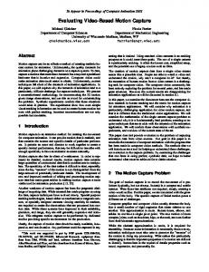
In this subsection we describe how one particle is corrected based on the auxiliary information. We first convert the − → four Euler angles into the 3D position of the elbow, E , − → and hand, H , respectively. We do this conversion for two reasons. Firstly, more smooth trajectories can be expected for these parameters and hence, better motion models can be defined. Secondly, we can directly apply the CoG to correct the predictions which is not so easy in the Euler − → angles representation. After this conversion both E and − → H are predicted using a linear first order motion model [11] and then kinematic constraints are applied to ensure a possible configuration [11]. First we will show how the prediction of the hand, − → H , is corrected and hereafter we will show how the pre− → dicted position of the elbow, E , is corrected. In figure 1 the predictions are illustrated using subscript ’p’ while the corrected predictions are illustrated using subscript ’c’. We assume a calibrated camera and can thou span a line in 3D, l, via the CoG and the camera, see figure 1. We can therefore correct the prediction by project−→ ing the predicted position of the hand, Hp , to the line, l. −→ The projected prediction is denoted H1 and calculated as −→ − → −→ − → − →− → − → − → H1 = P + ((Hp − P ) · F )F where P and F are the
Y
Hc
E1
Au
Ec
X
H1
Hp
Ep l
Z Figure 1. The shoulder coordinate system seen from above. The circle arc illustrates the sphere that defines the possible positions of the elbow. The large dashed line illustrates a camera ray through the hand. See the text for a definition of the parameters.
− → − → line parameters of l. P is the focal point and F is the vector spanned by the focal point and the position of the hand in the image, i.e., a direction unit vector. −→ We randomly diffuse H1 to account for the uncertainties in the estimate of the CoG. Concretely we first randomly draw a value from a Gaussian distribution with mean −→ −→ −→ in H1 and standard deviation = c · ||Hp − H1 ||, where c is a predefined constant. This point defines the displace−→ ment along the camera ray wrt H1 . The resulting point is −−−−→ now rotated around the vector H1 Hp using Rodriques’ formula [2]. The number of rotated degrees is determined by randomly sampling from a uniform distribution. The final −−−−→ diffusion of the point is along the vector H1 Hp . The dis−→ placement is define wrt H1 and designed so that the max−→ −→ imum probability is at H1 and that the tail towards Hp is more likely than on the opposite side. This corresponds to a Poisson distribution with its maximum probability lo−→ cated in H1 . We implement this by combining two Gaus−→ sian distributions, G1 and G2 , each with mean in H1 . G1 −→ represents the distribution on the opposite side of Hp and its variance is controlled by p(hand|bi ). G2 represents the −→ distribution on the same side as Hp and its variance is con−→ −→ trolled by both ||Hp − H1 || and p(hand|bi ). In praxis we first choose from which side of the mean we should draw a sample and then draws it from the appropriate (one-sided) Gaussian distribution. After these three diffusions we have the final cor−→ rected particle, denoted Hc . The difference between the predicted and corrected particles yields a measure of the −→ −→ −→ prediction error: He = Hc − Hp . The predicted position of the elbow can not directly be corrected by the auxiliary information. However, we know the elbow is likely to have a prediction error closely related to that of the hand as the hand and elbow are part of
the same open-looped kinematic chain. We therefore cal−→ culate the corrected position, Ec , by first adding the prediction error of the hand to the predicted value of the elbow, −→ −→ −→ yielding E1 = Ep + He , and then finding the point clos−→ est to E1 that results in a legal configuration of¯the ¯¯− ¯ arm. In −→ ¯¯ → −→¯¯ mathematical terms Ec = arg min ¯¯E − E1 ¯¯ subjected − → E ¯¯− ¯ ¯ ¯¯−−−→¯¯ ¯¯ →¯¯ ¯¯ ¯¯ to the constraints ¯¯E ¯¯ = Au and ¯¯EHc ¯¯ = Al . The solution to this problem can be found in [11].
4
The Observation PDF
For each blob, bi , we estimate an observation PDF and use this to weight the particles related to a particular blob. For the T · N particles that are not related to a blob we use the less accurate approach of chamfer matching instead of equation 3. The distance transform is calculated on the edge image in figure 2. The observation PDF in equation 3 is based on the orientations of the arm segments in the image. We estimate the PDFs of the orientations of the upper arm, pu (θu ), and lower arm, pl (θl ), respectively, based on edge pixels. As our input images contain background clutter and nontrivial clothes we utilize temporal edge pixels4 . That is, we find the edge pixels in the current image using a standard edge detector and AND this result with the difference image achieved by subtracting the current- and the previous image, see figure 2.B for an example5 . Those pixels actually belonging to the arm will be located in four classes, two for the upper arm and two for the lower arm, respectively. Our system does not impose restrictions on the clothes of the user. The clothes will in general follow gravity, hence the two classes of pixels originating from the upper sides (wrt gravity) of the upper- and lower arm will model the structure of the arm better, see figure 2.B. We therefore only consider temporal edge pixels located on the ”upper” sides. Concretely we define ”upper” and ”lower” via two lines described by the position of the shoulder in the image, the CoG of the blob, and the predicted position of the most plausible elbow location found among the most likely in the previous frame. We wish to estimate pu (θu ) and pl (θl ) independently and therefore separate the temporal edge pixels into two groups by calculating the perpendicular distance from each pixel to the two lines. As the prediction of the position of the elbow is uncertain we ignore all pixels within a certain distance from the predicted position of the elbow. Furthermore, we ignore all pixels too far away from both lines. When no predictions are available we use chamfer matching (as described above) as the observation PDF. Estimating the orientation of a straight line from data can be carried out in different ways, e.g., via principal com4 We
assume that only ego-motion is present. only a few temporal edges can be found we conclude that no motion is present and do not update the state-space parameters, i.e., no processing beyond this point is carried out. 5 When
A
B
Figure 2. A: A typical input image. B: The temporal edge pixels.
Altogether the stop criterion is found as the smallest n for which inequality 12 is true. To speed up the calculations the variance is not recalculated after each new sampling, but rather for every 10th sampling. Using the above described procedure we obtain two independent PDFs, one for the upper arm, pu (θu ), and one for the lower arm, pl (θl ). Different number of samplings might have been used to estimate the two PDFs. The accumulated probability mass for each PDF is therefore normalized to 1.
5 ponent analysis or linear regression. However, as we will not model the distribution of the orientations via Gaussians we can not apply these methods. Instead we apply the dynamic Hough transform (DHT). It estimates the likelihood of each possible orientation, hence allowing multiple peaks in the observation PDF. The choice of the DHT is furthermore motivated by the fact that it adapts to the data. The DHT randomly samples two pixels from one group and calculates the orientation of the line spanned by the two pixels. The more times the groups are sampled the better the estimation of the PDFs will be. On the other hand many samplings also lead to large processing time. The sampling of one group is therefore terminated as soon as the variance of the PDF is stable. To evaluate the stability of the variance after n samplings the variance of the last j variances is calculated as 2 νjn =
n 1 X 2 (σ − µjn )2 j i=n−j i
(10)
where σi2 is the variance after i samplings and µjn is the mean of the last j variances. The stop criterion is defined as the number of samplings, n, where the last j samplings are within the interval [µjn − λ, µjn + λ]. The distribution of the last j variances will in general follow a Uniform distribution. The theoretical variance of such a distribution in the given interval can be estimated as λ2 /12 [13]. When the mean of the variances, µjn is large it indicates large uncertainty in the PDF, which again indicates weak lines in the temporal edge image. A stable variance for such a PDF tends to required a larger value of λ compared to an image with stronger lines. To account for this difference λ is defined wrt µjn as λ=
µjn γ
(11)
where γ is found empirically. Setting the estimated √ variance equal to the theoretical variance yields λ = νjn 12. Inserting this result into equation 11 and writing it as an inequality yields 2 νjn ≤
µ2jn 12 · γ 2
(12)
Results
The effect of applying auxiliary information is illustrated by comparing this approach to a standard SMC-tracker. For both algorithms 50 particles are applied. After tracking the arm for 100 frames the characteristics of the two algorithms are illustrated in figure 3. First we illustrate the values of the predicted particles in the standard SMC algorithm (figure 3.A) and the values of the corrected particles when auxiliary information is applied (figure 3.B). We do not visualize all four parameters in the state-space but rather the 3D position of the hand projected into the image. In figure 3.B the main parts of the particles are located around the segmented skin-colored blobs and especially around the hand6 . These more focused particles result in a higher probability of finding the pose of the arm - even when using as few as 50 particles. This can also be seen in figure 3.C and 3.D where the three particles with the highest weights7 are illustrated in 2D for the standard SMC algorithm (3.C) and when applying auxiliary information (3.D). It can be seen that the auxiliary information improves the results. In images such as the one in figure 2.A the posterior PDF is in general ambiguous and a ”ridge” will be present in the posterior PDF. This means that a number of correct poses, i.e., poses that can explain the current image data, can be found by increasing the distance between the hand and camera, that is, moving along the ridge. This tendency can be seen in figure 3.D while the standard SMC algorithm fails to capture this tendency.
6
Discussion
In this paper we have suggested how to improve the SMC algorithm when dealing with articulated chains such as a human arm or leg. Our approach is based on the idea of applying auxiliary information from the current frame to correct the predicted particles. Comparing our approach to the standard SMC algorithm shows that we obtain more focused particles since our importance function is much more −→ −→ accurate than just using p(Xt |Xt−1 ). Furthermore, the 6 Note that the face blob is eliminated by feature, f . The neck region 1 is segmented into a different blob and therefore associated with some particles. 7 Highest weight first: black, white, thin black.
References [1] T.J. Cham and J.M. Rehg. A Multiple Hypothesis Approach to Figure Tracking. In CVPR, Fort Collins, Colorado, USA, June 23-25 1999. [2] J.J. Craig. Introduction to Robotics. Mechanics and Control. Addison Wesley, second edition, 1989.
A
B
[3] L. Davis, V. Philomin, and R. Duraiswami. Tracking Humans from a Moving Platform. In ICPR, Barcelona, Spain, September 3-8 2000. [4] J. Deutscher, A. Blake, and I. Reid. Articulated Body Motion Capture by Annealed Particle Filtering. In CVPR, Hilton Head Island, South Carolina, June 13-15 2000. [5] A. Doucet, N. Freitas, and N. Gordon, editors. Sequential Monte Carlo Methods in Practice. Springer, 2001.
C
D
Figure 3. The results of running the SMC algorithm with (B and D) and without (A and C) auxiliary information. See the text for details.
auxiliary information also allows the algorithm to quickly (re)initialization when the body part (re)enters the field of view. This is only the case for the standard SMC algorithm when a special (re)initialization procedure is added. One could argue that we should let the auxiliary information be a part of the observation PDF and then characterize our approach as a multiple cue (skin color and edges) approach. However, this is not the primary novelty of our approach. Instead the primary novelty is the concept of correcting the particles so that the SMC algorithm is more likely to find the true state-space parameters and hence require fewer particles when tracking an object. The core of our approach is to let the end-effector of an articulated chain be the auxiliary information. This is a sound concept, but requires a reliable detection of the endeffector. Skin color is in general a good approach for finding the hand. However, if the lighting changes significantly, for example in an outdoor setting or the user is wearing a Tshirt, this approach may fail. Therefore shape information should be incorporated to provide more reliable measurements of the hand. Furthermore, if the articulated chain is the human leg, skin color might not be the obvious choice when detecting the foot! Our observation PDF is quite different from standard approaches as we actually calculate the entire PDF as opposed to calculating it for only the particles that needs to be weighted. That is, we require relatively much processing estimating the PDF but the weighting is then trivial, see equation 3. Which is better depends on the observation PDF.
Acknowledgments This research is in part funded by the ARTHUR project under the European Commissions IST program (IST-200028559). This support is gratefully acknowledged.
[6] M. Isard and A. Blake. CONDENSATION - conditional density propagation for visual tracking. International Journal on Computer Vision, 29(1):5–28, 1998. [7] M. Isard and A. Blake. ICONDENSATION: Unifying Lowlevel and High-level Tracking in a Stochastic Framework. In ECCV, Freiburg, Germany, June 2-6 1998. [8] J. MacCormick and M. Isard. Partitioned Sampling, Articulated Objects, and Interface-Quality Hand Tracking. In ECCV, Dublin, Ireland, 2000. [9] R. Merwe, A. Doucet, N. Freitas, and E. Wan. The Unscented Particle Filter. Technical Report CUED/FINFENG/TR 380, Cambridge University, Engineering Department, 2000. [10] J. Mitchelson and A. Hilton. From Visual Tracking to Animation using Hierarchical Sampling. In Conference on Model-based Imaging, Rendering, image Analysis and Graphical special Effects, Rocquencourt, France, 10-11 March 2003. [11] T.B. Moeslund. Computer Vision-Based Motion Capture of Body Language. PhD thesis, Laboratory of Computer Vision and Media Technology, Aalborg University, Denmark, 2003. [12] T.B. Moeslund and E. Granum. A Survey of Computer Vision-Based Human Motion Capture. Computer Vision and Image Understanding, 81(3), 2001. [13] S.M. Ross. Introduction to Probability and Statistics for Engineers and Scientists. Wiley Series in Probability and Mathematical Statistics, 1987. [14] Y. Rui and Y. Chen. Better Proposal Distributions: Object Tracking Using Unscented Particle Filter. In CVPR, Kauai Marriott, Hawaii, December 9-14 2001. [15] C. Sminchisescu and B. Triggs. Covarinace Scaled Sampling for Monocular 3D Body Tracking. In CVPR, Kauai Marriott, Hawaii, December 9-14 2001. [16] Z. Zeng and S. Ma. Head Tracking by Active Particle Filtering. In FGR, Washington D.C., USA, May 20-21 2002.