For coherent motion M t will be zero, whereas for incoher- ent motion it ..... Stein, Anders Carlsson, Larry Snyder, Charles Anderson, and. Tim Holy for ... 15, 305. (1998). [21] J. R. Cavanaugh, W. Bair, and J. A. Movshon, J. Neurophysiol.
PHYSICAL REVIEW E 70, 031907 (2004)
Motion-contrast computation without directionally selective motion sensors B. K. Dellen, J. W. Clark, and R. Wessel Department of Physics, Washington University, Saint Louis, Missouri 63130, USA (Received 16 March 2004; revised manuscript received 6 May 2004; published 21 September 2004) The detection of relative motion, i.e., motion contrast, has been reported for motion-sensitive neurons in several vertebrate systems, yet the mechanism underlying motion-contrast sensitivity remains unknown. An algorithm for computing motion contrast directly from the moving intensity distribution is proposed. In this algorithm, the time-dependent intensity distribution of the visual space is convolved with a periodic function. For coherent motion, the resulting convolution integral reduces to a traveling wave of fixed amplitude, while incoherent motion causes the amplitude to oscillate. The frequency of the amplitude oscillation provides a measure of motion contrast. The algorithm is successful in reproducing tuning curves derived from measurements of motion-contrast sensitivity in avian tectum and primate middle temporal area. DOI: 10.1103/PhysRevE.70.031907
PACS number(s): 87.19.Bb, 87.19.Dd, 87.18.Bb, 87.18.Sn
I. INTRODUCTION
To function successfully in its environment, an animal requires the ability to distinguish a salient moving object from its background in the visual scene. In particular, it must be able to eliminate irrelevant whole field motion due to body, head, and eye movements. Self-evidently, motioncontrast detection, and its analog extension to motioncontrast estimation, are computational tasks of fundamental importance to visual processing in vertebrates. A large body of experimental evidence has established that visual processing of local image features is shaped by the context within which local features are presented [1–3]. Contextual influences on visual processing extend to higherorder image properties, such as image motion [4,5], which plays an essential role in the perception of visual scenes [6]. In the neural substrate, the contextual influences on image motion processing are represented by neurons whose response to two moving stimuli within their receptive field depends on the relative direction of motion between the two stimuli [7–13], an effect known as motion-contrast sensitivity. Specifically, the response is typically suppressed when the two stimuli move in the same direction, but the response is maximal when the two stimuli move in opposite directions, with intermediate responses for intermediate relative directions. The mechanism subserving motion-contrast sensitivity remains a mystery. The underlying computation requires spatial comparison of visual signals, presumably mediated by lateral and/or feedback connections [1,4]. Here we propose an algorithm for motion-contrast sensitivity that could plausibly be implemented by lateral connections. Unlike earlier mechanistic descriptions of the effect [14–16], the model developed here does not employ directionally selective motion sensors as elementary units. In Sec. II, we introduce a basic filtering process and show analytically that this filter is sensitive to motion contrast in the image. Section III presents simulation results in support of the analytical arguments. In Sec. IV, the algorithm is extended to two dimensions. We apply the motion-contrastsensitive filter to a variety of visual stimuli and compare its responses with experimental data from both pigeon optic tec1539-3755/2004/70(3)/031907(7)/$22.50
tum and middle temporal area of the monkey (area MT). In Sec. V we discuss the model against the background of existing models of motion-contrast sensitivity and experimental data. We further suggest an implementation of the model in terms of a neural network that might be realized biologically. II. MODEL
Our model employs a basic filtering process to sense contrasting motion in visual scenes and to determine the relative velocity of moving objects. The time-dependent, onedimensional visual input I共x , t兲 along the x dimension is convolved with a cosine function, leading to a transformed intensity distribution J共X,t兲 =
冕
I共x,t兲cos关k共X − x兲兴dx,
共1兲
L
where k represents a parameter of the transformation, and L is the distance over which the convolution is performed. Every point x of the visual space is assigned a cosine function I共x , t兲cos关k共X − x兲兴. The superposition of all the resulting cosine functions yields a transformed intensity distribution J共X , t兲 that is also a cosine function. A snapshot of this transformation is illustrated in Fig. 1 for the simple intensity distribution consisting of two points of light. Each of these point stimuli is represented by a cosine function that moves with the point. The spatial location of a given luminous point is lost under the postulated transformation, but information on relative motion is preserved. Superposition of the cosine functions from all points in the visual scene represents the salient information about the motion in the dynamics of the interference pattern. Using standard trigonometric relations and introducing the spatial Fourier transform Fk关I共x , t兲兴 of the visual input I共x , t兲, Eq. (1) is rewritten as J共X,t兲 = 兩Fk关I共x,t兲兴兩cos关kX − 共t兲兴,
共2兲
where
70 031907-1
©2004 The American Physical Society
PHYSICAL REVIEW E 70, 031907 (2004)
DELLEN, CLARK, AND WESSEL
ReFk关I共x,t兲兴 =
冕
Ia共x − vat兲cos共kx兲dx = a cos共kvat + ␣兲,
L
共6兲 where a=兩
冕
Ia共y兲exp共iky兲dy兩 = 兩Fk关I共x,t兲兴兩
共7兲
L
and
␣ = arctan
Im Fk关Ia共y兲兴 Re Fk关Ia共y兲兴
共8兲
,
while ImFk关I共x , t兲兴 is given by the same expression (6) with cos replaced by sin. The phase defined in Eq. (4) must therefore satisfy tan a = tan共kvat + ␣兲, FIG. 1. Schematic of the wave transformation. Two points of light of different intensity, represented by sharp peaks in the intensity distribution I共x , t兲 in the visual space at xa and xb, are transformed into cosine functions with amplitudes I共xa , t兲 and I共xb , t兲. The superposition of the cosine functions leads to a new intensity distribution J共X , t兲 = I共xa , t兲cos关k共X − xa兲兴 + I共xb , t兲cos关k共X − xb兲兴.
Fk关I共x,t兲兴 =
冕
so we may choose a = kvat + ␣. The transform (2) becomes Ja共X,t兲 = a cos共kX − kvat − ␣兲.
L
and
共t兲 = arctan
ImFk关I共x,t兲兴 ReFk关I共x,t兲兴
共4兲
.
共10兲
By symmetry, the same result applies for the transform of Ib, with a and ␣ replaced by quantities b and  defined from Ib共x − vbt兲 in analogy with Eqs. (7) and (8). Returning to the case where the moving intensity distributions Ia and Ib are simultaneously present, linearity of the convolution operation may be exploited to construct the total transformed intensity, to obtain
共3兲
I共x,t兲exp共ikx兲dx
共9兲
J共X,t兲 =
冕
I共x,t兲cos关k共X − x兲兴dx
L
Written in this way, the transform J共X , t兲 is seen to describe a traveling wave with an amplitude equal to the absolute value of the Fourier transform of I共x , t兲 at k. More explicitly, let the visual scene I共x , t兲 be composed of the sum of intensity distributions Ia共x , t兲 and Ib共x , t兲 that move rigidly with velocities va and vb, respectively, i.e., I共x,t兲 = Ia共x − vat兲 + Ib共x − vbt兲.
= a cos共kX − kvat − ␣兲 + b cos共kX − kvbt − 兲. 共11兲 As expected, this is a superposition of two waves traveling with velocities va and vb, providing the opportunity for interference. Alternately, this result may be cast in the form (2),
共5兲
J共X,t兲 = A共t兲cos关kX − ⌽共t兲兴,
We consider the two distributions individually, then superpose. With the distribution Ia = Ia共x − vat兲 present alone, we have
共12兲
where
再
A共t兲 = 兩Fk关I共x,t兲兴兩 = 共a − b兲2 + 4ab cos2
冋
⌽共t兲 = 共t兲 = kvat + ␣ + arctan
冋
k共vb − va兲t  − ␣ + 2 2
册冎
1/2
册
b sin关k共vb − va兲t +  − ␣兴 . a + b cos关k共vb − va兲t +  − ␣兴
031907-2
,
共13兲
共14兲
PHYSICAL REVIEW E 70, 031907 (2004)
MOTION-CONTRAST COMPUTATION WITHOUT…
The amplitude of the transformed intensity J共X , t兲 is seen to oscillate with a frequency f = k共vb − va兲 / 4, while the factor cos关kX − 共t兲兴 describes a carrier wave. Motion contrast within the visual field, as represented by the input (5), can therefore be directly determined from the frequency of the amplitude oscillation, which thereby provides a suitable measure of motion contrast. In the absence of contrast, i.e., if the motion of the two intensity components is coherent and va = vb, the amplitude A共t兲 is constant in time and the frequency is zero. As an instructive and important example, we consider two identical but independently moving test spots. Thus, the two moving intensity distributions are functionally identical, Ia共兲 ⬅ Ib共兲, which implies that a = b and ␣ = . The transformed intensity distribution (2) then collapses to
冉
J共X,t兲 = 2a cos k
冊 冉
冊
vb − va vb + va t ⫻ cos kX − k t−␣ . 2 2
共15兲 In this simple case we see immediately that for coherent motion (va = vb), the transformed intensity distribution is a traveling wave with constant amplitude that propagates with the velocity va of the test spots. On the other hand, for incoherent (opposing) motion 共va = −vb兲, the transformed intensity distribution, J共X , t兲 = 2a cos共kvat兲cos共kX − ␣兲, is a standing wave with an oscillating amplitude. The frequency f of the amplitude oscillation is given by f = k共vb − va兲 / 4 = kva / 2. We may note already at this point that a peculiar situation arises if either a or b is equal to zero in Eq. (13). Such a situation is realized for identical background objects that are at a distance that is an odd multiple of the half-wavelength / k of the convolution. The amplitude A共t兲 of J共X , t兲 is then constant, and contrasting motion with va ⫽ vb will not cause the amplitude of J共X , t兲 to oscillate. Accordingly, relative motion would be falsely perceived as coherent motion, creating a visual illusion. III. MOVING INTENSITY DISTRIBUTIONS IN 1D
In the proposed model for motion-contrast discrimination, the amplitude of the wave describing the transformed intensity distribution J共X , t兲 oscillates with a frequency proportional to the relative velocity of the moving constituents of the visual scene. The relative velocity is determined by measuring the frequency of the amplitude oscillation. To implement simulations to test the model, we apply a simple scheme. (i) Integrate the absolute value of J共X , t兲 over a multiple of the transformation wavelength = 2 / k to extract the time-dependent amplitude ˜J共t兲 = 兩A共t兲兩
冕
2m/k
兩cos关kX − ⌽共t兲兴兩dX,
共16兲
0
where m is an arbitrary integer. This quantity is independent of the spatial variable X, by construction. Taking the absolute value of a real function corresponds to a full-wave rectifica-
tion. Full-wave rectification requires a threshold operation with respect to both negative and positive values and can be implemented by synaptic connections 关17兴. Note that this step of the algorithm can in principle be replaced by a halfwave rectification. (ii) Next, we evaluate the amplitude modulation function, defined as M共t兲 =
d˜ J共t兲. dt
共17兲
For coherent motion M共t兲 will be zero, whereas for incoherent motion it executes an oscillation about zero with a frequency proportional to the motion contrast of the visual scene 关note that the oscillation frequency of M共t兲 differs from the oscillation frequency of A共t兲 by a factor 2, since the absolute value is taken in Eq. 共16兲兴. (iii) Finally, determine the frequency of the oscillation of M共t兲 to high accuracy from the power spectrum of the temporal Fourier transform of M共t兲. The spatial resolution of the computation is 0.1 deg, and the temporal resolution is 0.0125 s. The spatial frequency k of the transformation is 0.5 cycles/ deg. In the neural system, the parameter k corresponds to the spatial frequency of the motion-contrastsensitive neuron. Tectal neurons are band-pass spatially tuned with a maximum at about 0.5 cycles/ deg [18,19]. Spatial frequencies of neurons in monkey area MT range from 0.1 to 8 cycles/ deg [20]. The second important parameter of the convolution is the length L over which the convolution is performed. This parameter corresponds to the spatial extent of the nonclassical receptive field of the motion-contrastsensitive neuron. The total length of integration of the motion-contrast-discrimination algorithm is L = 80 deg, which lies within the experimentally established range for nonclassical receptive field sizes [5]. First, we apply the algorithm so defined to a visual scene consisting of two test spots of the same intensity [see Fig. 2(a)], each moving with a velocity of 8 deg/ s through the visual field of the detector. For t = 关0 , 3.8兴s, both stimuli are moving with the same speed and in the same direction. The amplitude modulation M共t兲 is zero. At t = 3.8 s, the direction of motion of one of the test stimuli is reversed and the two stimuli are now moving against each other. As a result, M共t兲 oscillates with a frequency of f = 8 Hz. The algorithm correctly determines the relative velocity to be 䉭v = 2 f / k = 16 deg/ s. Second, the algorithm is applied to a solid moving object of uniform intensity that moves in front of a random-dot background [see Fig. 2(b)]. This visual scene is chosen to correspond with experiments performed for neurons in the avian optic tectum [12]. The object size is taken as 5 deg of the visual field. The random dots, of size 0.1 deg, have a density of 1 dot/ deg. The visual field of the detector spans a visual angle of 80 deg. For t = 关0 , 3.8兴s, object and background are moving in the same direction with an absolute velocity of 8 deg/ s. This is an example of whole-field motion. The amplitude modulation remains predominantly at zero, with some fluctuations attributable to edge effects. Dots moving in and out of the visual field disturb the convolution
031907-3
PHYSICAL REVIEW E 70, 031907 (2004)
DELLEN, CLARK, AND WESSEL
standard deviation demonstrates that the algorithm leads to a robust and accurate computation of the relative velocity for a variety of complex stimuli.
IV. MOVING INTENSITY DISTRIBUTION IN 2D
The algorithm is readily extended to the physical case of two dimensions. Let us assume to be definite that there are two constituents of the intensity distribution in the visual space whose rigid motion is determined by velocity vectors v1 and v2, respectively. Suppose first that the visual scene projects onto an axis making an angle ␥ with v1. Then the velocity components parallel to the projection axis are v1␥ = 兩v1 兩 cos ␥ and v2␥ = 兩v2 兩 cos共␥ + ␦兲, where ␦ is the angle between v1 and v2. In analogy with the one-dimensional case, we convolve the projected, one-dimensional scene with a cosine function. The frequency of the amplitude modulation of the convolution integral will then be f共␥, ␦兲 =
k 1 k 1 兩 v 1␥ − v 2␥兩 = 兩兩v1兩cos ␥ − 兩v2兩cos共␥ + ␦兲兩. 2 2 2 2 共18兲
For ␥ equal to zero and for 兩v1 兩 = 兩v2兩, Eq. (18) reduces to f共␦兲 =
FIG. 2. Amplitude modulation M共t兲 as a function of time for different stimuli in one dimension. (a) Two test spots (black squares) move with absolute velocities of 8 deg/ s through the visual field of the detector. For t = 关0 , 3.8兴s, both stimuli are moving with the same speed and in the same direction. The amplitude modulation M共t兲 is zero. At t = 3.8 s, the direction of motion of one of the test stimuli is reversed, so that the two stimuli move against each other. As a result, M共t兲 starts to oscillate with a frequency of f = 8 Hz. With a spatial frequency of k = 0.5 cycles/ deg, the algorithm determines the relative velocity to be 䉭v = 2 f / k = 16 deg/ s, the correct result. (b) A solid object 5 deg in length moves in front of a random-dot background of density 1 dot/ deg. For clarity of presentation, every point of the 1D stimulus is represented by a vertical line in the image icon. Both object and background are moving with an absolute velocity of 8 deg/ s. For t = 关0 , 3.8兴s, object and background are moving in the same direction. The amplitude modulation remains predominantly at zero; fluctuations are caused by dots moving in and out of the visual field. At t = 3.8 s, the motion of the background is reversed, and the amplitude modulation starts to oscillate with a frequency of f = 8 Hz. Again, the algorithm determines the relative velocity to be 䉭v = 2 f / k = 16 deg/ s, the correct result.
given by Eq. (1) in an unpredictable way. At t = 3.8 s, the motion of the background is reversed and the amplitude modulation oscillates with a frequency of f = 8 Hz. The algorithm correctly determines the relative velocity to be 䉭v = 2 f / k = 16 deg/ s. Repeating the analysis for different random background patterns, we obtained the result ¯f = 8.008± 0.0681Hz for the average frequency. The small
k 1 兩v1兩兩1 − cos ␦兩, 2 2
共19兲
which specifies the tuning curve for relative object motion with respect to a projection axis parallel to the direction of v 1. To measure motion contrast independently of an absolute direction of motion (specified by ␥), one may repeat the motion analysis for two perpendicular projection axes, ␥ and ␥ + 共 / 2兲, and define an averaged frequency of amplitude modulation by
冉
f 2D共␦兲 = f共␥, ␦兲2 + f ␥ +
,␦ 2
冊 冉 冊 2
=
k 4
2
兩v1 − v2兩2 . 共20兲
For 兩v1 兩 = 兩v2兩, we obtain f 2D =
2k2 兩v1兩2共1 − cos ␦兲. 共4兲2
共21兲
Equations (21) and (19) have the same dependence on the angle ␦ between v1 and v2. Therefore, when the magnitudes of v1 and v2 coincide, Eq. (21) is valid both for motioncontrast detection with respect to an absolute direction of motion and for motion-contrast detection independent of an absolute direction of motion, apart from a constant scaling factor. Based on the extended model in the form developed above, the frequency tuning curve for a solid object moving in front of a random-dot background has been determined from computer simulations with the following specifications. The object size is chosen to be 5 ⫻ 5 deg2 of the visual field. The random-dot background spans the whole visual field of the detector 共80⫻ 80 deg2兲. Again the dot size is 0.1
031907-4
PHYSICAL REVIEW E 70, 031907 (2004)
MOTION-CONTRAST COMPUTATION WITHOUT…
FIG. 3. Comparison of the 2D model results with measured 2D tuning curves for motion-contrast-sensitive neurons. The visual stimulus consists of a solid object of size 5 ⫻ 5 deg2 and a random-dot background that spans the whole visual field of size 80⫻ 80 deg2. The density of the dots is 1 dot/ deg2 (inset). The random-dot background moves to the right (large gray arrow). The relative direction of motion ␦ between object and background is varied by changing the direction of motion of the object from −180 to +180 deg in steps of 45 deg. For an object moving in front of a moving random-dot background, the theoretical curve, proportional to 1 − cos ␦ (solid line), and the results of the simulations (filled black circles) reproduce the experimental tuning measurements from primate cortical area MT [10] and avian tectum [12,13]. Both the model results and the measured tuning data are normalized to their respective maximum values.
⫻ 0.1 deg2 while the dot density is 1 dot/ deg2. The relative direction of motion ␦ between object and background is varied by changing the direction of motion of the object from −180 to +180 deg in steps of 45 deg. To detect the motion contrast, the 2D visual scene is projected onto an axis parallel to the direction of the background motion and processed with the motion-contrast-detection algorithm established in Sec. III. The resulting frequency values may be used to construct a tuning curve that is normalized to the maximum response attained. The analytical tuning curves given by Eq. (21) and the response data representing experimental tuning curves for avian tectum [12,13] and cortical area MT [10] are normalized in the same fashion and plotted in Fig. 3, together with the normalized simulation results. The predictions from both analysis and simulation show excellent agreement with the experimental data. V. DISCUSSION
We have proposed a wave-interference algorithm of motion-contrast computation without motion sensors. The algorithm classifies the visual scene into coherent and incoherent motion and determines the relative velocity of the two moving parts of the visual scene. Most importantly, the 2D extension of the algorithm predicts the measured response to motion contrast as a function of the relative angle of object motion from avian tectum and primate area MT. Tuning to relative direction is usually found to be slightly broader than tuning to absolute direction of motion [21,22]. The algorithm is related to Fourier-based approaches of motion computation and, therefore, in general, it does not compute the rela-
tive velocity of non-Fourier or second-order-motion stimuli [23], which also appear to be largely ineffective stimuli in human relative-motion processing [23–27]. Even in early neural processing, local stimuli seem to be interpreted within the context in which the stimuli are embedded [1]. Neuronal responses to stimuli within the classical receptive field are modulated by stimuli from beyond its boundaries, i.e., from the nonclassical receptive field [5]. Motion-contrast sensitive cells present striking evidence for contextual influences from the nonclassical receptive field. Surround effects have been observed in the frog [7], the fly [8], and the cat, in the area MT [9], and the superior colliculus [10] of the monkey [11], in the avian optic tectum [12,13], and in the retina [28]. Most previous models of motion-contrast sensitivity have assumed that the mechanism underlying sensitivity to relative-motion direction involves an inhibitory interaction between directionally selective motion-sensitive cells [14–16]. However, it has been shown that responses of neurons are independent of the absolute direction of both surround and test stimuli [11,12]. This very fact casts doubt on the premise that directionally selective motion sensors must be an integral part of a motion-contrastsensitive neural network. It has been shown previously that sensitivity to speed contrast in the retina can be achieved without using directionally selective motion sensors as building blocks [28]. In this earlier work, sensitivity to speed contrast is explained by a model of retinal circuitry that involves pooling over nonlinear interneurons. However, given that this model only depends on speed, not on direction of motion, it does not account for relative-direction sensitivity of neurons in higher visual centers.
031907-5
PHYSICAL REVIEW E 70, 031907 (2004)
DELLEN, CLARK, AND WESSEL
FIG. 4. Neural implementation. A layer of spatial subunits (layer 1) gives input to a layer of linear summing units (layer 2) in a periodic way. Each subunit of layer 1 responds to motion within its receptive field (gray line). For a small moving object, this gives rise to a wave of neural activity (gray line) that spans the neural population of layer 2. When the object moves along the dimension of layer 1, the wave of activity will move with the point along the neural population of layer 2. Thus, the amplitude of the wave will oscillate in response to motion contrast. The population response is then rectified, integrated, and presented to an appropriate temporal filter h共t兲 to read out the oscillation frequency.
Here, we have demonstrated that motion-contrast sensitivity can be achieved without using directionally selective motion sensors as building blocks. In the model introduced here, all spatial information is discarded. Instead, motion-contrast sensitivity arises from global properties of the convolution
FIG. 5. Thought experiment. Two bars in the background are moving together against an object in the foreground. For t = 关0 , 1.2兴s, the bars are at a distance d that is an even multiple of the wavelength of the convolution integral. In this case, the superposition of the cosine functions representing the two bars leads again to a cosine wave that will interfere with the cosine wave representing the foreground object. As a consequence, the response of the detector will oscillate with a frequency that encodes the relative velocity between the background bars and the foreground objects. At t = 1.2 s, the background bars are moved at a distance that is an odd multiple of the half wavelength of the convolution integral. In contrast to the previous case, the cosine waves emerging from the bars will superpose to zero. Hence, the cosine wave representing the foreground object does not interfere with the background and the response of the detector will fail to oscillate even though motion contrast is present in the image. Thus, incoherent motion is falsely perceived as coherent motion.
integral (1). Before the convolution, the spatial separation of visual objects prevents a comparison of their motion properties and thereby frustrates the detection of motion contrast. The problem of spatial separation of the objects is overcome by transforming their local intensity pattern into a periodic function that integrates intensity signals from the whole visual field. Contrasting motion gives rise to a time-dependent modulation of the overall intensity distribution in the convolved visual space. The resulting oscillation contains information about the relative velocity of objects in the visual scene. Relative-motion sensitivity originates from interference of traveling waves that represent the moving objects of the visual space. Patently, wave interference is not restricted to cosine waves. Hence, the cosine function of the convolution integral (1) might be replaced by other functions, for example a wave function that has been constructed from a Gabor function. The proposed model is thus a global theory of relative motion; it does not compute local motion properties. As required, the model exhibits invariance with respect to wholefield motion. However, it does not distinguish between different types of relative-motion stimuli, for example a counterphase grating versus an object that moves in front of a background, nor does it filter out temporal modulation of the overall intensity of the image. The proposed algorithm can be implemented in a variety of plausible ways. For example, a set of spatial subunits (layer 1) could be connected to linear summing units (layer 2) in a periodic pattern (see Fig. 4). As a consequence, each neuron in layer 2 has a large, periodic spatial receptive field that resembles a cosine function. When an illuminated object moves through the visual field, it will cause an excitatory response (gray line) of the neural population of layer 1. The neural activity of layer 1 will produce a wave of neural activity spanning the population of neurons in layer 2 as a result of the periodic connectivity. This wave of activity will move with the stimulus through the population, thus implementing the convolution integral defined by Eq. (1). Finally, the population response of the layer-2 neurons is rectified, integrated, and temporally filtered to read out the frequency of the oscillation induced by motion contrast. This network architecture might require the participation of horizontal cells, such as exist both in avian tectum [29,30] and in mammalian cortex [2], to connect distant neurons.
031907-6
PHYSICAL REVIEW E 70, 031907 (2004)
MOTION-CONTRAST COMPUTATION WITHOUT…
The periodicity inherent in the convolution opens the possibility of an experimental test of the proposed algorithm that is suggested by the anomalous feature noted at the end of Sec. II. In principle, the perception of moving visual objects can be extinguished by convolving them with a periodic function. For arbitrary intensity distributions, this is unlikely to happen. However, an exceptional case can arise if two identical bars are chosen for the background. If the background bars are at a distance that is an odd multiple of half the wavelength characterizing the convolution integral defined by Eq. (1), the bars will eliminate each other. As a result, contrasting motion between an object and the background will be perceived as coherent motion. In an experiment designed to observe this phenomenon, one could sys-
tematically vary the distance between the background bars and determine whether the response of motion-contrastsensitive neurons is suppressed for certain distance choices when the background moves in opposition to a test spot (see Fig. 5).
We thank Ali Mahani for useful suggestions and Paul Stein, Anders Carlsson, Larry Snyder, Charles Anderson, and Tim Holy for comments on the manuscript. The work was supported by grants from the Whitehall Foundation, the McDonnell Center for Higher Brain Function, and NSF Grant No. PHY-0140316.
[1] T. D. Albright and G. R. Stoner, Annu. Rev. Neurosci. 25, 339 (2002). [2] C. D. Gilbert, Physiol. Rev. 78, 467 (1998). [3] K. Nakayama and J. M. Loomis, Perception 3 (1), 63 (1974). [4] T. D. Albright, in Visual Motion and Its Role in the Stabilization of Gaze (Elsevier, Amsterdam, 1993). [5] J. Allman, F. Miezin, and E. McGuinness, Annu. Rev. Neurosci. 8, 407 (1985). [6] K. Nakayama, Vision Res. 25(5), 625 (1985). [7] U. Grusser-Cornels, O. Grusser, and T. Bullock, Science 141, 820 (1963). [8] R. Virsik and W. Reichhardt, Naturwissenschaften 61, 132 (1974). [9] P. Hammond and D. M. MacKay, J. Physiol. (London) 319, 431 (1981). [10] J. M. Allman, F. Miezin, and E. McGuiness, Perception 14, 105 (1985). [11] R. M. Davidson and D. B. Bender, J. Neurophysiol. 65(5), 1115 (1991). [12] B. J. Frost and K. Nakayama, Science 220, 744 (1983). [13] H. J. Sun, J. Zhao, T. Southall, and B. Xu, Visual Neurosci. 19 (2), 133 (2002). [14] O. J. Gruesser, Vision Res. 3, 103 (1971). [15] T. Poggio, W. Reichhardt, and K. Hausen, Naturwissenschaften 68, 443 (1981).
[16] W. Reichhardt, M. Egelhaaf, and A. Guo, Biol. Cybern. 61, 327 (1989). [17] K. Graubard and D. K. Hartline, Science 237, 535 (1987). [18] O. Hardy and D. J. Gerschenfeld, Brain Res. 199, 452 (1980). [19] V. Porciatti, R. Alesci, and P. Bagnoli, Visual Neurosci. 2, 137 (1989). [20] L. P. O’Keefe and J. A. Movshon, Visual Neurosci. 15, 305 (1998). [21] J. R. Cavanaugh, W. Bair, and J. A. Movshon, J. Neurophysiol. 88, 2547 (2002). [22] R. T. Born, J. Neurophysiol. 84, 2658 (2000). [23] C. Chubb and G. Sperling, J. Opt. Soc. Am. A 5, 1986 (1988). [24] P. Cavanagh and G. Mather, Spatial Vis. 4, 103 (1989). [25] B. A. Dosher, M. S. Landy, and G. Sperling, Vision Res. 29, 1789 (1989). [26] M. S. Landy, B. A. Dosher, G. Sperling, and M. E. Perkins, Vision Res. 31, 859 (1991). [27] S. Nishida, M. Edwards, and T. Sato, Vision Res. 37, 199 (1997). [28] B. P. Ölveczky, S. A. Baccus, and M. Meister, Nature (London) 423, 401 (2003). [29] O. Hardy, N. Leresche, and D. Jassik-Gerschenfeld, J. Comp. Neurol. 233, 390 (1985). [30] H. Luksch and S. Golz, J. Chem. Neuroanat 25, 185 (2003).
ACKNOWLEDGMENTS
031907-7