Motion control of robot manipulators under sensor ...

Proceedings of the jrd World Congress on Intelligent Control and Automation

June 28-July

2,2000, Hefei, P.R. China -

.

Motion Control of Robot Manipulators Under Sensor Failure J. Gu and M. Meng

Al. Cook

Dept. of Electrical and Computer Engineering University of Alberta Canada T6G 2G7

Faculty of Rehabilitation Medicine University of Alberta Canada T6G 2G4

Abstract-There are robot dynamics and sensor fault, modeling error, system noise and measurement noise in a robot control system. How to control t h e robot manipulator under such circumstances to have good performance is presented in this paper. This paper addresses several techniques to control the robot manipulator under the uncertainty model and sensor failure. First a neural network is proposed to control the robot to follow the generated path. This network model is able to compensate the structured and unstructured dynamic uncertainties of the robot by using both on-line and off-line training. PD controller, com- ’ puted torque controller and adaptive controller with and without exact model are used to control the robot and compared with the proposed method. Second a residual generator for detection and isolation of the senor failure is designed. Assume one fault a time, the proposed method can detect and isolate the fault sensor. The simulation study based on a 2-d.0.f planar robot is included.

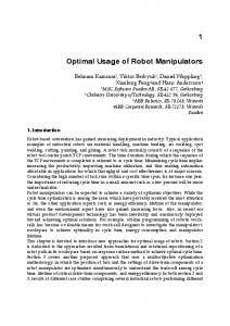
I. INTRODUCTIOIS To reach a specific target, the robot should follow the trajectory with controller. There are lots of studies of the control aspects of a robot [l,21. An ideal robot control system is difficult to achieve. There are environment noise, modeling error and faults which will effect the robot system as shown in fig. 1). It is difficult to control the robot

ation to achieve precise control. Computed torque controller needs the exact model to have good performance. Adaptive controller can deal with the robot under uncer tainty model. There are lots of studies of robot control under uncertainties using neural networks [3, 41. Meng [5] proposed efficient neural network architecture for iden tification and adaptive control of unknown robot dynamics. These controllers can achieve precise control and compensate partially unknown manipulator dynamics, but i t needs the online estimation of the robot dynamics and can’t deal with the sensor failure, which will be considered in this paper. Sensor failure detection methods have been presented since the 1970s. Many of these methods can be found in the three survey papers published by [6,7, 81. A fault detection scheme is composed in two steps: residual generation and residual evaluation. After the residual IS generated, statistical test can be carried out to detect and isolate the failure. This paper begins with a proposed neu ral network, which can control and compensate partially unknown manipulator dynamics. Next a PCA (Principle Component Analysis) based parity space residual genera. tion and Chisquare test algorithms are used to detect and isolate the sensor failure. The results of the simulation are presented and the control algorithms are compared with ea& other. The paper concludes with the discussiorl and further considerations 11. PARTIALLY UNKNOWN ROBOT MANIPULATOR CONTROL

A one-layered feed forward neural network is designed for motion control of robot manipulators. A. Model for motion control of robot manipulators

The dynamics of an n d.0.f rigid robot manipulator can be described by Fig. 1: A

typical robot control system with uncertainties

under uncertainties. Classic PD controller doesn’t require the model of the robot, however, it needs the large actu-

M(qYi + 4 q , 4

* 4 + G(q) = 7

I 1‘I,

Where T is the .vector of joint torques; q, q, and q are the joint position, velocity and acceleration, respectively; M , C and G represent the mass, velocity and gravity terms,

A . Parity space approach

respectively. Equation (1) can also be expressed as [5]

Mq

+ C * q + G = Y(q,o,d)* 0 = 7

(2)

Where Y 6Rnxris a coefficient matrix consisting of known function of q, q, and g, which is called manipulator regressor, and @ERrX' is a vector consisting of known and unknown robot dynamic The control law is assigned as 7 = Y ( Q , d , &*) 6 - K3 (3) Where qr = 4 - A * 6 , s = q - qr, e = q - qr and K and A are a c:nstant matrices (for more detail, see Meng, [5]). Variable 0 can be expressed as

Q=G+A0

(4)

Where 6 is obtained by an off-line learning process using a recursive error back propagation process [9]. A 0 is updated using an on-line learning process,

A 6 = -rYTs

(5)

Y=WX

(7)

Consider a measurement equation y = Hx

+ Ay + E

(10)

Where y E RQ is the measurement vector. H ( q x n ) is the measurement matrix, x E R" is true measurement value, and Ay E RQ is the error vector, E is the uncorrelated measurement noise with unit variance. Let a q x (q - n) matrix v be determined such that

vTH = 0

(11)

vTv = Iq-n (12) One of the methods of calculating the matrix v is Potter's algorithm [lo] Hence p =vTy = vT(H2

+ Ay) = vTHz + vTAy = vTAy

(13)

The above equation reveals that the parity equations conWhere r is a constant matrix Choosing a L~~~~~~~ tain only the errors due to the faults. columns of vT define q distinct fault directions associated with each measurefunction ment. i.e. the ith column of uT determines the direction 1 along which p lies if Ay = Ayi = [O .. . OAyO .. . OIT. = - ( s T ~+ s (Q- o)Tr-1(8 - 0)) ( 6 ) This will ensure that a fault in measurement i implies a 2 It is proved that the position and velocity tracking error growth Of p in ith direction* converge to zero [5]. The off-line training-process & be 3. Statistical hypothesis test expressed as

,

Where Y +T, X+Y (q, q, ci;) and W+0. The weight W is updated by wm

= W,4+

(1-XT,P,

-1

xm)-'(Y,-Wm-1

The variable P is updated by

y = H x + Ay + E fault happened ~ = H x + E fault free Xm)XmT Pm- I (8) The tests are following:

{

Ho : E[p] = 0

+

Pm= Pm-i (1 -XT,p,-iXm)-lPm-lXm)X,TPm-i Where x m = tails, see [9].

[Xm-lixmli ym

=

[um-l,yml.

From previous section, p of parity equation residuals is determined. Two hypotheses are identified as Ho,the normal mode, and H1 , the failure mode. The equations of the two hypotheses are following

{ H1 E[p] = Ay :

(9) For de-

111. SENSOR FAILURE DETECTION OF ROBOT MANIPULATOR CONTROL SYSTEM

(14)

fault f ree E[(p- AY)(p - AY)T] = vuT fault (15) E[ppT] = V V T

The log likelihood ratio A ( p ) for the two hypothesis is given by A(p) = 1/2[pT(~vT)-'p- ( p - A Y ) ~ ( v ~ ? ' ) - '( PAy)]

A fault detect scheme is composed in two steps: residual generation and residual evaluation.

(16) The maximum likelihood estimate Ag of Ay is the value which maximize the expression:

Hence,

Afi = Ay

74

(18)

Substituting this into j? yields the detection decision function

vT = [ V I , v2 . . .v*-n] The isolation decision function

B. PCA based sensor. failure detection When PCA is applied to monitoring the performance of an process, the squared prediction error Q (161 is usually used. The Q statistic is given by:

-

Qh = Z T ( I PD~PZ~)Z (25) z is the new data to be monitored. The upper limit for

(20)

the

Given p, a failed sensor is identified by computing the n values of the decision function. If DFrk is the largest of these values, then the kth sensor is the one which-is mostly likely to have failed. More about this can be found in [ll].

Q statistic is given by,

Where c, is the normal deviate corresponding t o the upper lOO(1- a)th percentile.

IV.USE PCA MODEL TO GENERATE THE PARITY MATRIX AND DETECT THE FAILURE

m

A . Parity matrix generation and

For a robot system, the feedback will be the joint position, joint velocity and joint acceleration. So for m d.0.f robot, there will be m x 3 vectors.! lets call it X

x = [e1e2 ... e, dl e, ... e, el e, ... i,]

Where Ai is the eigenvalue of the correlation matrix related to data x.

The PCA model can be shown as follows:

X = TPT + E = TPT + f'PT = [TFI[PPIT

(22)

[Tq is orthogonal and [PPI is orthonormal. The dimension of P (Dp)is the number of principle components. A.

The relationship between P and

P is

[PP][PP]T= PPT e PPT = I

V. SIMULATION STUDY Yhjectory generation P

For simplification without losing generalization, a t w e degree of freedom (d.0.f) planar robot is used for simulation study. The length of the two links is chosen as l m and the point mass of each link is 2k, and lk, respectively. The desired trajectory is an ellipse with the horizontal axis length 1.5m and the vertical axis lm respectively. Using inverse kinematics, the joint space [e of the robot tracking the whole ellipse is obtained. The trajectories of the robot in joint space and Cartesian space are shown in fig. 2 .

(23)

1 is identity matrix.

When the model isapplied to the new data, the residual p will be

P

e4

(24)

Trajectory in Cartesian Space

Tm)ectory in Joinl sp.ce

1

= P'PTZnew( t )

KOWassume Z n e w ( t ) = zO,,,(t)+AZnew(t), wherez:,,(t)

>

is true value, and the Axnew(t)is fault value respectively. It is ~ a s to y find out that PTz&,,(t)-O., Then the primary residual can be defined p = P T A Z n e w ( t ) , here v = pT. This primary residuaf can be used for the hypothesis test. It can also bo used to isolate the faulty sensor by using incident matrlx Interested readers are referred to [12, 13, 14, 151.

0 o 5 m l

4 5 -1 -2

- 81

0

-1

0 X

1

2

-"o

200

400 Time

Fig.3fCartSan space and joint space

75

800

EM

B. Using the proposed neural network controller to control the robot under uncertainty os

Using proposed neural network architecture; several computer simulations have been done with motion control of robot manipulators. To control the robot to follow the generated trajectory shown in the left panel of fig. 3, the desired velocity and acceleration of the desired trajectory are obtained by using the inverse Jacobian and the derivative of the inverse Jacobian. Then, the neural network is trained off-line using the recursive error back propagation process. The weights are referred to the manipulator regressor is given by

-1

0 X

1

200

0

400

800

Boo

Time

Fig. 4: The trajectory and error dynamics using neural network controller. The left panel shows the simulated trajectory in comparison with the desired trajectory. The error dynamics is shown in the right panel.

BT = [m21112 m2b2 m212 (ml +m2)11 (ml +m2)1l2] (29) torque controller and adaptive controller are used to conThe true value of ml and m2 are 2 and 1 respectively, the true value of ZI and 22 are 1 respectively. The initial of BT is chosen randomly. After three steps, the final error is less than After learning, the manipulator regressor is [1.001.00 1.00 3.00 3.001, and the true values is [l 1 1 3 31, which is exactly the same with the trained results as shown in fig. 3.

trol the robot to follow the desired trajectory. First, a PD controller is used. fig. 5 shows the error dynamics of the joint angles. Various gains are tried t o test the PD controller, and when K p = 200 and kv = 10, the controller can achieve a better result. The steady state error of the joint angles 81, 8 2 are 7.5256" and 2.7662O, respectively. Dynamics Error of

--I\

PD

I

0

200

400

600

800

Time Iteration Times

'

Fig. 5: The error dynamics of joint angles using a PD controller

Fig. 3: The error dynamics of off-line training.

Then the weight obtained via off-line training process is used as the initial values for the adaptive on-line training whose learning algorithm is described in (7-9). The initial position, velocity and acceleration is chosen 95% of the desired initial values, respectively. In addition, a disturbance [l 1IT is added t o the model. The dynamics of the trajectory in workspace is shown in the left panel of fig. 4. The right panel of fig. 4 shows the error dynamics of two joint angles. The steady-state error of 81 , 8 2 are -0.1600° and O.O337O, respectively. It shows that proposed model can follow the generated trajectory very well.

c. The comparison of joint dynamics with other controller To see how well the proposed model performs, several other control approaches, such as PD controller, computed

76

Then, computed controller with and without exact robot configuration model is used. The left panel of fig. 6 shows the error dynamics of joint angles using computed torque controller with exact model. The steady state error of the joint angle 81,8 2 are -0.1913O and -0.3656", respectively. This result is better than that using a PD controller, but is not azj good a the proposed model. Using a computed torque controller with model mismatch by multiplying a constant 0.4 to M ( 8 ) matrix, the error dynamics of the joint angles is shown in the right panel of fig. 6. The steady state error of joint angles 01, O2 are -0.4831O and -0.9453", respectively. Finally, an adaptive controller is used to control the robot to follow the trajectory shown the left panel of fig. 7. The adaptive controller uses the compute torque control and takes advantage of the manipulator regressor of the robot dynamics. There is a model mismatch; the initial

'

missed detection probability. Using (19,25, 26, 27, 28), the thresholds for both methods are obtained, and the results are shown in fig. 8. The algorithm in section IV.B (right panel of fig. 8 ) is more conservative than the one in section 1II.B (left panel of fig. 8). -4

0

2 0 0 4 m 8 w B w

Fig. 6: The error dynamics of joint angles using a computed torque controller with exact model (left panel) and model mismatch (right panel).

value of ml and ma are set as 0.8 and 0.4 respectively. The true value of ml and ma are 2 and 1respectively. The Fig. 8: Sensor data under normal operation steady state error of the joint angles 81, 82 are -0.1036O and -0.1363O respectively. The results of the adaptive controller are better than the PD controller and computed 2) Simulation resufkp for sensor failure torque model, and is as good as the proposed model. To simulate the failure of the aensor, fault vectors arr added to the sensor d a t a The exemplar is divided intc six periods. The faulty vector is added to the first, thin Error Dynamics Using Adaptive Control and fifth period. For the W period, the faulty vector i added to the second sensor, for the third period, the h u l t vector is added to the fourth s e m r , and the fifth period the faulty vector is added to the sixth sensor. Using th technique in section I11 and IV,the sensor is detected ant isolated as shown in fig. 9. It is clear that the hulty dat is detected and isolated.

e 7

Fig. 7 The error dynamics of joint angles using an adaptive controller.

U)

3

Ba

ij4

10

D.Sensor failure

detection and isolation

1 ) System under n o n n a l operation During the simulation, the data block will be z,,,, m = 6 is the number of th,e feedback vector, and n is number of samples. Here n is chosen as 628. Assume at first the data are all good. There is no fault at this time. Through analysis the data, the correlation matrix is obtained, the eigenvalues are found and the residual space is obtained using (23,24), which is the IJ in parity space:

[

2

-0.02ii -0.0004

-o.oeis

o.asra o.8iia

-0.a8ee o.4aso

o.sm

-0.0000

0.80'19

0.DTTP

0.1431

0.0014

-o.smo

-0.0087

O.SIOI

o.im

0.3108

]

In this case, the threshold is a upper percentage point of X a ( 3 ) distribution for the given a = 0.1 which is the 77

Fig. 9: Sensor data under abnormal operation: Left side of ti panel shows the sensor failure detection. Right side shows the isol tion results

E. Robotics control under sensor failure The proposed algorithm and the sensor failure dete tion algorithm can be combined together, 80 that the sy tem can control the robot manipulators both under tl uncertainties and the sensor failure. fig. 10 shows ti block diagram of the system. The FDIA block means tl failure detection, isolation and accommodation. Accoi modation method is not presented in this paper becau

of the space limit of the paper. Model baaed estimation method is used for the estimation of the state vector during the simulation. During the simulation study, the same trajectory is used as the input of the system, at the same time mismatched robotics model is used, and the faulty vector is added to the output to simulate the sensor failure. The simulation shows that these two algorithms can be well combined together.

L. Jin and M. M. Gupta, “Dynamic feedback control of unknown nonlinear systems using dynamic neural networks,” in IEEE 1995 Intl. Conf. on Systems, Man and Cybernetics, pp. 1261-1266, IEEE, 1995. A. R. S. R. K. S. and A. 0. H., “Adaptive neural network for identification and tracking control of a robotic manipulator,” in IEEE 1995 Intl. Conf. on Systems, Man and Cybernetics, pp. 601-609, IEEE, 1995. Q.-H. M. Meng, “Application of an efficient neural network to identification and adaptive control of unknown robot dynamics,” Intl. J. of Intelligent Control ond Systems, vol. 1, no. 4, pp. 459-468, 1993.

R. Isermann, “Process fault detection based on modeling and estimation methods- a survey,” Automotico, vol. 20, no. 4, pp. 387-404, 1984. A. S. Willsky, “A survey of design methods for failure detection in dynamic systems,” Automotico, vol. 12, pp. 601-611, 1976.

Fig. 10: Robot control under both uncertainties and sensor failure

F’. P. M., “Fault diagnosis in dynamic systems using analytical and knowledgebased redundancy. a survey and some new results,” Automotica, vol. 26, no. 3,pp. 459-474, 1990.

VI. DISCUSSIONS AND FURTHER CONSIDERATIONS The proposed neural network controller takes advantage of the manipulator regressor and the recursive error back propagation learning algorithm, it can dynamically control the robot to follow a desired trajectory. For only three steps of iteration, the error goes to less than l.0em8. In addition, the on-line learning process will guarantee that the tracking position and velocity errors will converge to zero although initially there may exists a model mismatch. The proposed sensor failure detection algorithm combines the PCA model and the parity space approach together. It will detect the sensor failure when the faulty vector is added to the sensor data. The proposed neural network controller and the sensor failure detection algorithm can be built into the robot control system to do the control and sensor failure detection and isolation. The proposed models can be extended in the future work. Modifying its on-line learning process and removing its off-line learning process can improve the proposed model for motion control of robot manipulator. Also o p timal algorithm can be used to design the parity space to increase the probability of failure detection and isolation.

VII. REFERENCES L. W. S. and M. Q.H., uRegressor formulation of robot dynamics: computation and applications,” IEEE Zhnsoction on Robotics ond Automotion, pp. 323-333, 1993. C. study of model based and non-model-based trollers, “An enhanced computed-torque control robot manipulator with a neuro-compensator,” in Intl. Conf. on Syrtems, Mon ond Cykmetics,

robot conscheme for IEEE 1995 pp. 61-66,

IEEE,1995.

78

K. N. and V. A, “Efficient learning algorithms for neural networks,” IEEE ltonsaction on System, Man ond Cybernetics, vol. 23,pp. 1372-1383, 1993.

J. Potter and M. Suman, “Thresholdless redundancy management with arrays of skewed instruments,” Integrdy in Electronic Flight Contml Systems, vol. 15,pp. 1-25, 1977.

K. C. Daly, E. Gail and J. V. Harrison, “Generalized likelihood test for fdi in redundant sensor configurations,“ Joumol of Guidonce and Control, vol. 2, no. 1, pp. 9-17, 1979. J. Gertler and D. Singer, “A new structural framework for parity equation-based failure detection and isolation,” Automatico, vol. 2, pp. 381-389, 1990. J. Gertler and D. Singer, “Augmented models for statistical fault isolation in complex systems," in Proceedings of the 1985 American Control Confemnce, pp. 317-322, IEEE,1985. J. Gertler, “Survey of model-based failure detection and isolation in complex plants,” IEEE Contml systems mogosine, vol. 2, pp. 3-11, 1988.

Y.H. Janos Gertler, Weihua Li and T. McAwy, “Isolation enhanced principle component analysis,” AIChE Joumol, vol. 45, pp. 323-334, 1999. J. E.Jackson and G. Mudholkar, “Control procedures for residuals associated with principle component analysis,” Technometn’cs, vol. 21, pp. 341-349, 1979.