n ordered probit model is used to predict motor vehicle usage in Australia on the basis .... Of course a number of externalities also arise from motor vehicle usage ...
Toyota Motor Corporation Australia Ltd. - all of whom donated .... 94. 3.3.2
Effectiveness of short tests. 95. 3.3.3 Fuel consumption issues. 96. 3.3.4 Cost of
repairs and ...... an electric blanket placed adjacent to the tank. At the end of the
h
Sample Motor Vehicle Usage Procedure. 1. Overview of the Procedure. This
procedure is a staff guide for the use of [insert organisation name] company.
Inspection Manual includes the formal rules governing many facets of the
program, ... The current rules are a product of a project that began in late 2004.
..... AGENT means the owner or representative of a Sticker Replacement Station
or.
Maintenance control procedures. 9. ... TOYOTA FORTUNER. POOL. NIX 5298 ....
The responsibility for the repairs and maintenance schedule rests with the ...
Dec 6, 2008 ... Canada owes the success of its statistical system to a long-standing partnership
between. Statistics .... 2004, found that about 7 in 10 motor vehicle thefts were
reported to police, although this figure climbed to 89% .... the Hond
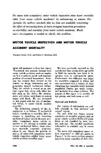
The strik- ing feature of Figure 2 is that for all four sex-race groups the motor vehicle accident mortality rate is higher in the noninspection compared with the in-.
Nov 28, 2016 - multi-year partnership agreement with Netball Australia. ... partnered with French manufacturer Renault u
12VALJ6680. $19.84 1994 PLYM VAN VOYAGER LE ... 07VWXX5362. $93.69
1999 JEEP CHEROKEE GRAND ... $33.64 2001 MITS MONTERO SPORT L.
Sep 9, 2013 ... Alliance, Mercedes-Benz, and Porsche request NHTSA to ..... derivatives of the
Sprinter platform will ..... files (2000–2009) indicate that frontal.
ESRC Centre for Business Research, University of Cambridge. Working Paper No. ... 1,800 claims of unintended acceleration incidents in the 1980s, Audi became ..... Figure 2: UK Recall Incidents and Number of Vehicle Recalls 1992-2002.
Aug 10, 2017 - completion of continuing education, as are required by the ... receive any license issued by the commissi
... Holden Ute VS III, Holden Ute VR and 4-wheel drive vehicles such as the
Toyota Landcruiser 70 Series, 80 Series, and Nissan Patrol are also popular
targets.
Refer to manufacturer's specifications for all tolerances. ✓. A torn C.V. boot, rack
and pinion boot, or ball joint boot is no longer a cause for rejection. ✓.
The Motor Carrier Services Commercial Motor Vehicle Guidebook is prepared
based on Indiana's laws and .... Inspections and Out-of-Service Orders . ..... the
driver: • A road tractor. • A tractor truck. International Registration Plan. (Plates .
MOTOR VEHICLE DIVISION (Central Office) ... This manual provides information
on how certain activities are performed and is ... Cavalier County Treasurer.
Late Assistant Professor, Mechanical and Electrical Engineering Department,. The Royal Military College of Science. W. S
INTERIOR OF VEHICLE. ✓Steering Wheel Bind and Play. ✓Brake Pedal Power-
Brake. Reserve. ✓Brake Warning Light. ✓Windshield Wiper Operation. ✓Mirrors.
persons who purchase, lease, or convert electric, plug-in hybrid electric, ... credit
for a plug-in hybrid electric conversion is $7,500. ...... 2010 Honda Insight.
-Chiyo and Strauss to be joined by Nissan V8 Supercar driver Rick Kelly in the #1 Nissan GT-R NISMO GT3
Media Information MICHAEL KRUMM AND LUCAS ORDONEZ IMPRESS IN MAIDEN NISSAN V8 SUPERCARS TEST MELBOURNE, Australia (August 13, 2013) – Michael Krumm and Lucas ...
Nov 28, 2016 - Having such a massive footprint across this country, from both netball and Nissan ... Email: peter_fadeye
n ordered probit model is used to predict motor vehicle usage in Australia on the ..... models estimating the decisions of the number, type and vintage of vehicles.
MOTOR VEHICLE USAGE PATTERNS IN AUSTRALIA: A COMPARATIVE ANALYSIS OF DRIVER, VEHICLE & PURPOSE CHARACTERISTICS FOR HOUSEHOLD & FREIGHT TRAVEL KATHLEEN GOFFEY & ANDREW WORTHINGTON Goffey, Kathleen and Worthington, Andrew (2003) Motor Vehicle Usage Patterns In Australia: A Comparative Analysis Of Driver, Vehicle & Purpose Characteristics For Household & Freight Travel. International Journal of Transport Economics 30(2):pp. 219-250. Copyright 2003.
n ordered probit model is used to predict motor vehicle usage in Australia on the basis of the unit record files underlying the Australian Bureau of Statistics’ Survey of Motor Vehicle Use. Both household and freight transport are analysed. The paper examines the statistical significance of a number of driver, vehicle and travel purpose variables on the level of motor vehicle usage. Factors analysed include driver age and gender, vehicle and fuel type, age of the vehicle, purpose of trip, place of registration, type of freight and number of drivers. The results indicate that the cut-off points between very low, low, medium, high and very high vehicle usages are significant and that the factors associated with differences in usage include driver age, engine size and age of vehicle for household vehicles and the type of freight, type of vehicle, gender and number of drivers for freight usage.
A
KEY WORDS: Motor vehicle usage, driver, vehicle and purpose characteristics, ordered probit. JEL CLASSIFICATION: D12, C21, C25, L92.
I.
INTRODUCTION
oad transport plays a major role in Australia’s economy and society. And fundamental to the provision of road transport is the usage of motor vehicles. Households use their vehicles for access to their places of work, education and recreation, while the use of vehicles by business is primarily for the movement of goods and the provision of services. However, and seemingly regardless of the now century long dominance of motor vehicles on Australian roads, motor vehicle usage continues to attract a significant amount of empirical attention by Commonwealth and state government departments, transport organisations, industry groups and academic researchers aimed at setting and implementing transport policy and determining road funding and investment. Justification for this ongoing interest is not hard to find, especially when in a country of Australia’s size road transport will continue to play a significant role in the efficient functioning of the economy for at least the foreseeable future.
R
Currently, the movement of people and goods by road in Australia takes place on more than 811,000 kilometres of road, with 84.4 percent of the network comprising local roads and 40 percent featuring a sealed surface (Austroads, 2000). The vastness of this road network is especially apparent in terms of the number of persons per kilometre of road, such that in Australia there are approximately 24 persons per kilometre of road, less than half the number found in comparable economies such as the United States and New Zealand (Austroads, 2000). Australia’s road infrastructure is currently valued in excess of $100 billion and requires significant ongoing building and maintenance expenditure by all levels of government and the private sector. For instance, in 2000-01 construction activity undertaken by public
2
MOTOR VEHICLE USAGE PATTERNS IN AUSTRALIA
and private organisations for the construction of roads, highways and bridges totalled $1.8 billion and $3.8 billion respectively (ABS, 2001d). In the year to October 2000 the total kilometres travelled by all vehicles in Australia was estimated at 180.8 billion kilometres (ABS, 2001a). While this represents only a slight increase from previous years, increasing amounts of road usage are concentrated on a smaller proportion of the road network. For example, while nearly 85 percent of the network constitutes local roads, these roads carry less than 25 percent of all traffic, with the remaining network comprising rural and urban arterial roads and national highways (Austroads, 2000). Likewise, within each state more than half of the average distance travelled per year occurs in the capital cities, as opposed to the provincial cities and non-urban areas (ABS, 2001a). And while the proportion of kilometres travelled for personal use has declined marginally over the last 20 years (from 48.9 percent in 1979 to 43.5 percent in 2000), the share of business travel has increased (from 32.2 percent in 1979 to 34.4 percent in 2000) as well as travel to and from work (from 18.8 percent in 1979 to 22.1 percent in 2000) (Austroads, 2000; ABS 2001a). The road network also plays a major role in freight transport. In 2000-01, freight movements by road accounted for 52.4 percent of the 1.2 billion tonnes of domestic freight uplifted, as compared to 43.5 percent for rail, 4 percent for sea and 0.01 percent for air (ABS, 2002a). However, since road freight transports high tonnages over relatively short distances, road’s share of total tonne-kilometres (mass moved over distance) is 29 percent when compared with 39 percent for rail and 32 percent for sea (ABS, 2002a). While road transport obviously represents a significant proportion of business costs, the cost of household road transport is also significant. In fact, private consumer transport expenditure represents some 16.9 percent of the household budget and comes second only to the proportion spent on food (ABS, 2000). Of this transport expenditure, the majority (73.7 percent) is spent on private motoring with the remainder on public transport (ABS, 2000). For example, the NRMA (1999) estimated that a medium sized car that is from new to 3 years old, travels approximately 15,000 kilometres per year, and was bought on a personal loan for 75% of the purchase price at an interest rate of 10.2% over four years costs the owner approximately $174.70 per week, excluding running and maintenance costs. Due to the high volume of transport services used in Australia, the transport industry itself contributes a significant percentage to overall economic activity. In 2000-01 the transport and storage industry was worth $31.6 billion, contributing 5.0 percent to total gross domestic product (GDP). Of the transport and storage industry’s contribution to GDP, the road transport sector accounted for 30 percent in this same period (ABS 2001c). In addition to representing a sizeable proportion of economic output, the industry currently employs approximately 4.4 percent of Australia' s labour force with over half of these jobs generated by the road transport sector (ABS 2002b). Significant amounts of turnover and employment are also accounted for by particular industries within this sector. For example, in 1999-00 turnover in operating buses for the transportation of passengers in urban areas and over long distances was estimated at $2.9 billion, with a labour force of nearly 35,000 people; operators of taxi cabs and hire cars generated turnover of $1.2 billion and employed over 10,000 people; the manufacturing of motor vehicles generated turnover of $13.1 billion, with a labour force of 15,693 people; motor vehicle retailing generated turnover of $21.9 billion and employed some 35,000 people; and firms engaged in retailing automotive fuel or lubricating oils provided turnover of $17.2 billion with the industry employing approximately 42,000 people. Of course a number of externalities also arise from motor vehicle usage including, pollution, congestion, and road traffic accidents, as well as the transport planning activities undertaken by government departments and transport organisations through the collection of road revenue and the infrastructure investment decisions and road expenditure undertaken. In terms of air pollution the Australian Greenhouse Office (AGO, 2001) estimated that Australia' s transport sector produced 16.1 percent of total CO2 equivalent emissions in 1999, with 90.2 percent of emissions produced by road transport, cars being the major contributor. Noise pollution and congestion are yet other problems associated with road transport that can have a number of effects on health and well-being (Button, 1994). Lastly, road accidents are a widely recognised undesirable consequence of road transport and include the costs
K. GOFFEY & A. WORTHINGTON
3
associated with deaths, injuries and damage to vehicles; currently estimated to cost $15 billion per annum (Austroads, 2000). Lastly, in order to build and maintain the largely publicly provided road transport network, as well as managing the externalities associated with its use, Commonwealth and state governments use the revenue collected from a number of taxes and charges levied on road users. In 1997-98 a total of $13.7 billion in revenue was generated by motor vehicle taxes, charges and fees for the Commonwealth and State governments (Austroads, 2000). For instance, the purchase of a new vehicle attracts a goods and services tax (GST) valued at 10 percent of the vehicle purchase price, a luxury car tax of 25 percent for vehicles over $55,000, vehicle ownership costs include annual registration charges, compulsory third party insurance, stamp duty (applicable on initial car registration, transfer of ownership and insurance), driver’s licence, and other charges specific to each State or Territory (Austroads, 2000). In terms of vehicle use, the Commonwealth levies an excise on leaded and unleaded petrol and diesel, toll charges are applicable on some roads in certain states. However, though road transport related revenue is indeed significant, only some fifty percent is currently outlayed by all levels of government directly for road related expenditure (Austroads, 2000). With these statistics in mind, the modelling of road transport usage can make an important contribution to understanding both the patterns of motor vehicle activity and the evaluation of policy, planning and operational initiatives aimed at improving efficiency and reducing negative impacts associated with road transport (D’Este, 2000). The purpose of the present paper is to investigate the role of driver, vehicle and usage characteristics in determining this pattern of motor vehicle usage. The paper itself is divided into four main parts. The first section provides a brief empirical survey of travel demand and vehicle usage models. The second section discusses the methodology and data to be employed in the paper. The results of the analysis are examined in the third section. The paper ends with some brief concluding remarks.
II. EMPIRICAL SURVEY (i) Aggregate and disaggregate travel demand models The empirical literature on motor vehicle usage lies within the broader field of transport demand modelling. Two main forms are recognised. First, aggregate travel demand models aim to represent the behaviour of a group of travellers through the estimation of aggregated data. Though initially developed in response to the realisation that travel choices are rarely identified separately (Hensher and Goodwin, 1979), these techniques have also been used for aggregating individual travel behaviour using microdata [see, for example, McFadden et al. (1977), Stubbs et al. (1980), de Dios Ortuzar and Willumsen (1994) and Train (2002)]. Aggregate demand functions can be further categorised as consistent or approximate, depending on the method used for estimation. The first type of aggregate demand is obtained by summing individual demand functions and is therefore considered to be most consistent with underlying demand. However, this type of demand function is difficult to estimate and is not widely employed (Train, 1986). The second, and more common, type of demand function are those that approximate the underlying aggregate function, but are not necessarily consistent with notions of realistic individual demand (Train, 1986). Second, disaggregate travel demand models focus instead on the choices of whether a travel journey should be undertaken in the first instance and by which transport mode in the second. Past research has examined a number of travel choice problems including the choice of destination, time of day to travel, level and type of car ownership, degree of vehicle usage and duration of vehicle ownership. Such models are generally regarded as the most appropriate for examining travel choice problems since these decisions are ultimately based on behavioural observations of individuals or households and theories of consumer choice and utility maximisation (Bitzios and Ferreira, 1997: 11). Within disaggregate travel choice models, three broad characteristics exist that further categorise this approach. These are (i) real or
4
MOTOR VEHICLE USAGE PATTERNS IN AUSTRALIA
hypothetical choice models, (ii) discrete or continuous choice models, and (iii) static or dynamic choice models. The first, real (or revealed-preference) or hypothetical (or stated-preference) choice models, depends on whether the household' s choice of travel is observed in a real situation or whether the household is asked what it would do in a hypothetical situation (Train, 1986). Of these, revealed-preference models are the common approach taken in modelling current transport usage patterns, whereas stated-preference models are associated with transport choices consumers have yet to experience (such as the demand for electric vehicles). The second types of disaggregate transport choice models relate to either discrete or continuous choice. Discrete choice relate to one-off decisions regarding transport (such as the level and type of vehicle ownership), whereas continuous choice refers to decisions made on an ongoing basis (such as vehicle utilisation). The third type of model is made on the basis of whether it contains static or dynamic elements. This is primarily related to the household vehicle ownership decision, since in the long run the vehicle ownership process is essentially dynamic, with static models focusing on a one off travel decision. Empirical studies involving the estimation of vehicle usage can be dated back to at least the mid 1960s where an aggregate model was estimated as a means of forecasting car ownership and use (Kain and Beesley, 1965). However, interest in vehicle utilisation models, especially disaggregate models, gained attention in the 1980s due to increased concerns for energy availability and fuel consumption emerging from the energy shocks of the 1970s (Mannering, 1983; Greene and Hu, 1984; Mannering and Winston, 1985; Hensher, 1985a). In the 1990s interest in household vehicle usage was renewed, this time as a result of interest in forecasting vehicle emissions and the demand for alternative-fuel and environmentally friendly vehicles (Golob et al., 1996; Golob et al., 1997; Bjorner, 1999). Past modelling of vehicle utilisation within these areas can be divided into three areas: (i) joint (continuous/discrete) decision models; (ii) vehicle utilisation within multi-vehicle households; and (iii) aggregate estimates of total distance travelled by passenger vehicles. (ii) Joint decision models Early travel demand models estimating the decisions of the number, type and vintage of vehicles generally failed to recognise the importance of the effect distance travelled by the household has on these transport decisions. That is, a household’s motor vehicle usage may impact upon its decision in regard to the number of vehicles owned. A vehicle' s fuel efficiency, which in turn is related to driving habits, may also influence the type of vehicle owned, and conversely the number and type of vehicles a household owns affects the frequency and distance the household members drive and hence the amount of fuel consumed (Mannering and Train, 1985). Many early studies either ignored the vehicle miles/kilometres travelled (VMT/VKT) or assumed it to be exogenous (Mannering and Train, 1985). An obvious alternative was the specification of joint decision models, including those undertaken by Train and Lohrer (1983) and later Mannering and Winston (1985). Using US household data, Train and Lohrer (1983) specified seven sub-models containing decisions regarding the number of vehicles to own (restricted to two vehicles), the class and vintage of each vehicle, the miles travelled in each vehicle (VMT) and the proportion of VMT by category of travel trip. Importantly, while these sub-models were estimated sequentially, this was not assumed to be the actual sequence in which households make these decisions. By comparison, Mannering and Winston' s (1985) joint decision model took into account the dynamic elements of automobile demand. The data utilised was collected over three periods, capturing purchasing and utilisation behaviour before, during and after the June 1979 energy shock (Mannering and Winston, 1985). Similar to Train and Lohrer (1983), separate models were estimated for one and two vehicle households based on the choice of vehicle quantity, type and utilisation. A later study by Hensher et al. (1990) used Australian multi-vehicle household data collected from the Sydney metropolitan area during 1981/82. In contrast to Train and Lohrer (1983) and Mannering and Winston (1985), Hensher et al (1990) specified a vehicle utilisation model that simultaneously considered vehicle type and usage choices. For households with two or more vehicles the model treated
K. GOFFEY & A. WORTHINGTON
5
each vehicle as a unique entity, similar to the earlier approach taken by Train and Lohrer (1983) and Mannering and Winston (1985). Hensher et al extended their study to estimate separate usage equations for households with 1, 2, 3 and 4 or more vehicles (Hensher et al., 1990). Despite several key differences, all three studies specified an array of household socio-economic, financial and locational variables as well as vehicle specific variables as determinants of vehicle usage. For example, for two vehicle households all three studies included a dummy variable indicating if the observational vehicle was the newer vehicle. Both Mannering and Winston (1985) and Hensher et al. (1990) concluded that households drive their newer vehicles more than the older vehicle. And in most other respects, the results of these three studies are comparable regarding the specification of the explanatory variables and the relationships between these and the level of household vehicle ownership. For instance, Train and Lohrer, (1983), Mannering and Winston (1985) and Hensher et al. (1990) all concluded that vehicle ownership was positively related to income, while household size (Train and Lohrer, 1983), the number of workers (Train and Lohrer, 1983; Mannering and Winston, 1985) and the expected number of miles/kilometres driven annually were also significantly positive. Conversely, operating costs (Train and Lohrer, 1983; Mannering and Winston, 1985 and Hensher et al. 1990), the age of the household head or primary driver (Mannering and Winston, 1985 and Hensher et al., 1990) and vehicle age (Hensher et al., 1990) all lead to a decrease in household vehicle use. Other results included Train and Lohrer’s (1983) finding that households in large urban areas drive more than households in small urban areas, and those in small urban areas drive more than households in rural areas. De Jong (1990), Linciano (1997) and Bjorner (1999) have also undertaken work in this area. Both de Jong (1990) and Bjorner (1999) used maximum likelihood methods to simultaneously model vehicle ownership and vehicle usage, taking account of both fixed and variable costs based on datasets from Holland and Denmark respectively. Linciano (1997) studied the vehicle usage decision conditional on vehicle ownership in the U.K., accounting for self-selectivity through the application of a probit model at the discrete choice stage and least squares estimation for the continuous choice, together referred to as the Heckman model. The results of these studies generally supported Train and Lohrer, (1983), Mannering and Winston (1985) and Hensher et al. (1990), while de Jong (1990) and Bjorner (1999) also concluded that a female driver or household head was associated with lower vehicle usage. Other developments in joint decision models have extended the estimation of joint decisions beyond vehicle ownership, type choice and usage. For example, Schimek (1996) estimated a model that studied the relationship between choice of residence, automobile ownership and automobile usage. The estimated model produced similar inferences to those of previous studies for the explanatory variables of income, household size, number of workers and driver age, and in addition found that an increase in population density would decrease the level of vehicle travel per household each year. Similarly, de Jong (1996) estimated decision models of vehicle holding duration, vehicle type choice and annual travel length, for Dutch households with initially one vehicle. The estimated parameters again supported comparable studies and also suggested that highly educated persons drove more kilometres. (iii) Vehicle usage in multi-vehicle households Research on how multi-vehicle households utilise each of their vehicles became popular amongst transport economists at the same time as joint estimation techniques. Mannering and Train (1985: 268) identify two interrelated concerns that form the reasoning behind modelling vehicle usage in multivehicle households. These are: “…(i) how to capture the process by which households assign vehicles to trip-generating activities, and (ii) how to account for the fact that household vehicles can be used as substitutes”. Mannering and Train (1985) argued in the first instance that the vehicle assignment process needed to consider the compatibility of vehicle attributes with household activities; that is, how vehicles are assigned for use between household members and the occurrence of individual vehicle ownership in the household. These same issues would also be addressed when considering the concept of vehicle substitutability in the second instance. It is interesting to note that while a number of joint decision studies also examined vehicle usage in multi-vehicle households, none of these explicitly addressed the
6
MOTOR VEHICLE USAGE PATTERNS IN AUSTRALIA
issue of vehicle substitutability as relevant to multi-vehicle household usage models (Mannering and Train 1985). Two early studies in vehicle usage in multi-vehicle households were by Mannering (1983) and Hensher (1985a). Mannering (1983) constructed a simultaneous equation system for two vehicle households that incorporated the occurrence of substitution across vehicles. Two models were estimated, one for each vehicle in the household, using a three-stage least squares simultaneous equation procedure. The data set applied was based on a three-month period, consisting of relatively few household socioeconomic and vehicle specific variables. However, due to the relatively short time period, Mannering (1983) was able to treat vehicle type attributes as exogenous as it was assumed that the possibility of changing vehicles during this time was unrealistic. Rather, if usage was to be considered over the long-term (i.e. a year) then vehicle type attributes would need to be viewed as endogenous which would necessitate the estimation of type and level choices jointly using discrete/continuous econometric techniques (Mannering, 1983). Mannering (1983) also highlighted the importance of the principal driver age variable suggesting that attributes of the principal driver provide a clearer indication of likely activity choices in which the vehicle is to be used and also accounts for some of the driver/vehicle associations thought to exist. Hensher’s (1985a) study on the influences on household vehicle use were based on a similar assumption in that the interdependence of vehicle use in a household was also assumed to be endogenous. Each vehicle was identified separately in the household observational unit and simultaneous equations were estimated using three-stage least squares. The over-riding difference between the two studies is that Mannering’s (1983) study was limited to two vehicle households in the short-run, whereas Hensher (1985a) extended his study to include up to three vehicle households over both the short-run and a 12month longer-run period. This same data set was later used in a joint decision study by Hensher et al. (1990), which took into account substitution between household vehicles. During the mid-to-late 1990s, vehicle usage research changed focus. Increasing emphasis was now placed on the environmental effects of vehicle emissions, which lead to a renewed interest in the need to forecast vehicle miles/kilometres travelled. Golob et al. (1996) and Golob et al. (1997) undertook studies in this respect where usage was considered a function of household characteristics, principal driver characteristics and characteristics of the vehicle. Principal driver characteristics specified included driver age, gender and employment status. However, Golob et al., (1997) also included information on consumers’ preferences for alternative-fuel vehicles, based on stated preference data, to obtain an idea of the extent to which households would use these environmentally friendlier vehicles over more conventional vehicles. Golob et al. (1996) and Golob et al. (1997) found that the age of both the first and second vehicles had a negative influence on VMT of each vehicle and on the other vehicle. In terms of vehicle types, it was found that vehicles with greater than average use included subcompact cars, sports cars, full-size vans, compact sport utilities and full-size sport utilities (both first and second vehicles), compact cars and small (compact) pickup trucks (second vehicle only). Mini cars and fullsize (standard) cars were estimated to have average usage levels and vehicles with lower than average use included full-size (standard) pickup trucks and minivans (both first and second vehicles), small (compact) pickup trucks (first vehicle only) and mid-size cars (second vehicle only). Golob et al. (1996) and Golob et al. (1997) also examined the impact of a number of household characteristics on VMT. Vehicle miles travelled was found to be also positively related to: (i) the number of household members between 16 and 20 years old, (ii) the total number of children, (iii) highincome households, (iv) households headed by younger persons and (v) the number of workers in the household. Further, positive effects on VMT came from the number of children in the household aged 1 to 5 years, however this was for the second vehicle only. Lower household vehicle usage was associated with the number of drivers in the household, retired households (both vehicles) and the presence of three or more household vehicles (second vehicle only). The negative influence of the number of drivers in the household was explained by both studies as indicating a shift of use towards third or fourth vehicles in the household.
K. GOFFEY & A. WORTHINGTON
7
(iv) Aggregate household vehicle usage models Aggregate models examining vehicle usage also date back to the mid-1960s (Kain and Beesley, 1965). However, studies treating vehicle usage as the endogenous variable remained a fairly untouched area of transport modelling until the rise in popularity of the disaggregate models in the 1980s. Rather, the earlier aggregate models required vehicle usage data as a means of estimating fuel consumption, instead of analysing the determinants of vehicle usage (Mannering, 1983; Hensher, 1985a; Hensher et al. 1990). Two recent aggregate vehicle usage studies include Walls (1998) and BTE (1998b). The study by Walls (1998) was motivated by the need to model usage of the existing fleet of cars in Hong Kong as an input to an overall congestion abatement strategy. With this in mind, VKT per automobile was posited to be a function of vehicle taxes, vehicle fees, petrol price, income and population. Least squares estimates indicated that vehicle taxes, vehicle fees and petrol prices were expenses directly related to the ownership and operation of the vehicle. By comparison, BTE (1998b) modelled vehicle usage that took into account distance travelled in capital cities and major provincial urban areas in Australia. City dummy variables were included to reflect the different levels of availability of public transport and/or differences in the propensity to travel by car within these regions (BTE, 1998b). The only other variable included in the model was implied VKT, measured as the product of trends in cars per thousand persons nationally, VKT per car nationally and the population of each city. Pooled time series, cross-section data and estimates using OLS and GLS provided negative values in Sydney, Melbourne and Brisbane, on which basis BTE (1998b) suggested the presence of factors such as high congestion levels and/or higher availability of public transport produced lower urban passenger vehicle VKT. BTE (1998b) predicted that passenger vehicle VKT in capital cities was expected to grow by 1.2 percent per annum from 1995 to 2020, compared to the observed growth rate of 3.5 percent from 1971 to 1995, with the difference assumed to be partly due to slower economic growth and increased saturation of car ownership. (v) Freight vehicle usage models Freight vehicles serve a very different purpose to passenger vehicles, as they are primarily associated with the movement of goods rather than people. Modelling freight demand and the movements of these types of vehicles can provide insights into the issues of traffic congestion, distribution patterns and routing, supply chain operations, and pricing and regulatory matters (D' Este, 2000). While the literature on freight demand modelling, both aggregate and disaggregate, is generally less extensive than passenger demand modelling, the topic has been of interest since about the mid 1970s, and formed the basis of a number of literature reviews [see, for example, Winston (1983) and Zlatoper and Austrian (1989)]. Two obvious problems with freight demand modelling studies identified by these surveys are the complexity in the pattern of freight movements and the problems associated with data collection, especially at the disaggregate level. Many of the techniques that have been applied to modelling freight transport have their origin in methods originally developed for passenger vehicles (D’Este, 2000). Consequently, the intended purpose for estimating road freight models are in some instances similar to passenger vehicles (i.e. mode choice) and in other cases very different (i.e. inventory analysis, firm profit, effects of regulatory change, etc.). And demand for freight movement models are usually estimated in terms of volume (tonnage), number of consignments or as direct vehicle trips rather than distance travelled (D' Este, 2000). However, a number of studies have incorporated road freight tonne-kilometre by commodity to estimate the energy use of road freight vehicles (Vanek and Campbell, 1999; Vanek and Morlok, 2000). De Dios Ortuzar and Willumsen (1994) found that the majority of freight demand models are of the aggregate form. In part, this can be attributed to their usefulness in estimating freight flows on a largescale (regional or national) for policy analysis or practical prediction (Winston, 1983) primarily for the purposes of examining modal choice (Winston, 1983; Zlatoper and Austrian,1989). One such aggregate modal choice model is the basic modal split model where modal share is dependent on the price and service differences between carriers. Another aggregate modal choice model developed in response to shortcomings of the aggregate modal split models by specifying the firm' s cost function to derive the
8
MOTOR VEHICLE USAGE PATTERNS IN AUSTRALIA
aggregate share of a mode by commodity group and by geographical region (Winston, 1983). However, de Dios Ortuzar and Willumsen (1994) and Winston (1983) recognised that both of these models had a drawback in that while aggregate models were able to provide insights into mode choice, at high levels of aggregation information on the process by which firms optimise their behaviour was lost. Similarly to passenger demand modelling, the estimation of freight demand by disaggregate methods has proven beneficial in capturing the characteristics of freight demand at the firm level. A literature review Winston' s (1983) identified two main types of disaggregate freight demand models, namely, behavioural and inventory. Winston (1983; 421-422) concluded: [B]ehavioural models attempt to focus on the mode choice decisions made by the physical distribution manager of the receiving or shipping form. The analysis is motivated by the proposition that the manager is concerned with maximising the utility, with respect to expense and service, he receives from using a given mode. ...inventory models have attempted to analyse freight demand from the perspective of an inventory manager, [that is] it implicitly attempts to integrate the mode choice and production decisions made by a firm. While inventory models have similar estimation methods to the joint choice models of passenger demand, Winston (1983) and later Zlatoper and Austrian (1989) highlighted the fact that conventional single choice models are theoretically less complete and more likely to be biased than the freight models that jointly analyse important endogenous choices. As with passenger vehicle studies, freight vehicle research in recent years has focused on the estimation of vehicle emissions and energy use. For example, Vanek and Campbell (1999) and Vanek and Morlok (2000) studied the road freight industry' s level of energy use from a commodity-based, rather than a traditional mode-based, perspective. In order to identify which industry sectors have the highest product-specific road freight energy intensity, both studies used information on road freight tonnekilometre and average energy use per tonne-kilometre. Vanek and Morlok (2000: 21) outlined the importance of this type of study, concluding "…firms defined by a commodity group can use this information to understand their sector' s contribution to freight energy use and, where the energy level is determined to be relatively high, set goals for reducing it". Vanek and Campbell (1999) likewise found that the food and drink sector was the largest consumer of road freight energy, followed by manufactured articles, building supplies and agriculture. Vanek and Morlok' s (2000) results analysed road freight energy intensity in comparison to the energy used in the production process for that commodity. They showed that foods and kindred products, lumber and wood products, and apparel had the largest transportation energy use components as compared with the energy used in the production process.
III. DATA AND MODEL ESTIMATION The analytical technique employed in the present study is to specify motor vehicle usage (both household and freight) as the dependent variable (y) in a regression with driver characteristics, vehicle attributes and purpose factors as explanatory variables (x). A large number of vehicle usage studies have employed limited dependent variable or discrete choice models for this purpose. Train and Lohrer (1983), Mannering and Winston (1985), Hensher et al. (1990) and de Jong (1996), for example, used logit for analysing fleet size and vehicle type choices. Likewise, Linciano (1997) specified a probit model for the discrete choice of car ownership with the application of least squares for the continuous vehicle usage data, while Bjorner (1999) used the tobit model in his estimation of the discrete/continuous choice of ownership and usage. Winston (1981a) used probit models to examine the demand for intercity freight transportation, and de Palma and Rochat (1997) employed a similar model to examine the impact of weather conditions on the travel decision. Accordingly, the following multinomial ordered probit model with simple heteroskedasticity is specified:
K. GOFFEY & A. WORTHINGTON
9
y i* = β *'x i + ε i ,
ε i ~ N [0, wi ], y i = 0 if y i* ≤ µ 0 , = 1 if µ 0 < y i* ≤ µ 1 ,
(1)
= 2 if µ 1 < y i* ≤ µ 2 , ... = J if y i* ≤ µ J −1 . where εi is distributed normally with a mean of zero and Var(εi) equals wi2. This model comprises a form of censoring. The µs are unknown parameters to be estimated with β. The coefficients imputed by the multinomial ordered probit provide inferences about the effects of the explanatory variables on the probability of the possible outcomes for vehicle usage. All data used in the study is from the previously unreleased unit record files underlying the Australian Bureau of Statistics Survey of Motor Vehicle Use. This survey collects data on passenger and freight vehicle usage where the unit of observation is the vehicle itself. Other information collected includes characteristics of the principal driver, the vehicle, usage patterns and for freight vehicles, the types of commodities carried. Data on passenger and freight vehicle movements collected over the 13-week period from 1 May to 31 July 2000 is specified and contains details relating to 752 passenger and 1,896 freight vehicles.
The dependent variable in both the passenger and freight vehicle analysis is vehicle kilometres travelled (VKT). Vehicles in the sample are categorised into quintiles on the basis of the reported distance travelled: namely, very low, low, medium, high and very high. The lower and upper bound of distances travelled for passenger and freight vehicles in each quintile are detailed in Table 1. For example, the medium level of usage for passenger vehicles is between 2,119 and 3,631 kilometres, while the medium usage for freight vehicles is between 4,415 and 8,432 kilometres. Three sets of explanatory variables are used to predict passenger and freight vehicle usage. These are: (i) driver characteristics, (ii) vehicle attributes, and (iii) purpose factors. Selected descriptive statistics are presented in Table 2. The first set of characteristics for both passenger and freight vehicle usage relate to driver characteristics. Within a behavioural travel demand model it is expected that the characteristics of the principal driver will have a significant influence on distances travelled. Mannering (1983), for example, argues that older drivers and women tend to select frequencies and types of activities that require less travel. Negative signs are hypothesised when vehicle usage is regressed against driver age (AGE) and gender (SEX) where the control variable for dummy variable is male. The number of vehicle drivers (HSE) is included to take account of the increasing scale of usage for each vehicle and in part proxies household size (Greene and Hu, 1984; Golob et al. 1996; Golob et al., 1997). In addition, as part of the driver characteristics for both the passenger and freight analyses, information on the state of vehicle registration serves to act as a proxy for residential or business location. Five dummy variables are specified with NSW as the control: Victoria (VIC), Queensland (QLD), Western Australia (WA), South Australia (SA) and other States and Territories (OTH) including the Northern Territory, Australian Capital Territory and Tasmania). Hypotheses could, of course, be made for each of the States or Territories with the level of usage related to say, land area or road length. Nevertheless, no particular a priori sign is hypothesised when vehicle usage is regressed against state/territory of registration.
10
MOTOR VEHICLE USAGE PATTERNS IN AUSTRALIA
Of course, there are a large number of other driver characteristics that could have been included in the analysis had the data set employed focused on the user rather than the vehicle. For example, Mannering (1983), Green and Hu (1984), Hensher (1985), Golob et al. (1996), and Linciano (1997) all included household income with the hypothesis that road transport as a normal good would be higher in highincome households. However, the evidence supporting this is mixed, with Golob et al. (1996) and Linciano (1997) regarding income as an important influence on vehicle usage, and Green and Hu (1984), Hensher (1985) and Hensher et al. (1990) concluding otherwise. Another driver/household characteristic included in past studies is geographical location, primarily delineated as urban or rural [see, for example, Train and Lohrer (1983), Mannering and Winston (1985), Linciano (1997) and Bjorner (1999)]. The underlying hypothesis in this respect is that the lower population density of rural areas, the distances to services, facilities, places of work and education, and the lack of public transport are associated with higher vehicle usage. The second set of characteristics specified as explanatory variables relate to the attributes of the vehicle itself. Vehicle attributes posited to have a relationship with vehicle usage in past studies include: vehicle age (Green and Hu, 1984; Hensher, 1985; Hensher et al., 1990; Golob et al., 1996; Golob et al., 1997; Linciano, 1997), operating costs (Train and Lohrer, 1983; Mannering and Winston, 1985; Hensher, 1985; Hensher et al., 1990; de Jong, 1996; Golob et al., 1996; Golob et al., 1997; Walls, 1998), and the cost of fuel (Greene and Hu, 1984; Linciano, 1997; Walls, 1998). Hypotheses underlying these variables include the fact that as vehicles age they become less reliable and efficient due to technology improvements and are consequently driven less, and that vehicles with higher operating costs would be used less in order to reduce costs incurred by households. The later is also expected to hold for the price of fuel, notwithstanding the generally inelastic demand for gasoline, diesel, etc. The set of explanatory variables in Table 1 reflect most of these concerns with the exception of fuel price. However, this is not considered a major limitation. For example, Linciano (1997: 450) argues “..the impact of changes in fuel prices on the individual transport behaviour is stronger only in the long term”. Information on different fuel types and consumption, however, has been included. For passenger vehicles it is hypothesised that leaded and mixed-fuel vehicles (LDF) will have a negative coefficient, as these petrol types are more common among older vehicles. The variable OTF representing diesel, LPG and duel fuel is hypothesised to have a positive influence on usage. Schipper et al. (2000) argue that the annual driving distances of vehicles with these fuels are significantly higher than those for gasolinefuelled vehicles. This positive relationship is also expected for the freight fuel variables DSL (diesel) and OTF (leaded, LPG, dual). Efficiency of operation is also reflected in part by the specification of the fuel consumption rate for both passenger and freight vehicles (RTE). The age of the passenger and freight vehicles is indicated by the year of initial registration (YRR) and year of manufacture (YRM) respectively. These variables would imply a higher and lower likelihood of usage due to lower and higher operating costs and positive and negative ex ante coefficients are hypothesised respectively. Several other variables are included to reflect additional vehicle attributes that may affect usage. In terms of the type or class of vehicle, Golob et al. (1996), Golob et al. (1997) and Hensher (1985) included vehicle types in their respective studies. The results suggested that vehicles associated with higher usage included subcompact cars, sports cars, full size standard vans and compact and standard sports utility vehicles. In contrast, lower usage is generally associated with mid-size cars, standard trucks and minivans. These are consistent with Golob' s et al. (1996) reasoning that vehicles with higher usage levels tend to be driven principally by males, younger persons and employed persons, whereas vehicles with lower usage levels are driven by females or as second household vehicles. Likewise, Linciano (1997; 450) included engine size on the basis that "…households who purchased a powerful vehicle might need to travel more extensively than those who brought a small car" and Hensher (1985) and Hensher et al. (1990) included variables indicating vehicle weight and whether the vehicle is used for towing. The present freight analysis includes a dummy variable for trailer towed (TLR) in this respect. For passenger vehicles, dummy variables are used to identify vehicle types as FVU (4WD, vans, utilities), TAX (taxis) and MOT (motorcycles), with sedans and station wagons as the
K. GOFFEY & A. WORTHINGTON
11
control variable. Due to the nature of work performed by taxis, it is hypothesised that TAX is positively related to vehicle usage, while motorcycles (MOT) generally travel a lower number of kilometres and are therefore likely to be negatively related to usage. The vehicle types for freight vehicles are LTK (light truck), RGD (rigid truck), PMR (prime mover) and OTH (other non-freight carrying), while the control group is freight-carrying passenger vehicles. Greene and Hu (1984), for example, also included a truck vehicle class, though it only included standard-sized pickup trucks, vans and recreational vehicles, rather than freight trucks. It is hypothesised vehicle usage (VKT) will have a positive coefficient when regressed against long-distance freight vehicles PMR and RGD and a negative relationship when regressed against LTK and OTH which tend to be used for shorter distance freight transport. Additional dimensions of vehicle attributes included are the number of cylinders (CYL) and engine capacity (ENG) for passenger vehicles and the number of axles (AXL) and gross combination mass (GCM) for freight vehicles. Vehicles with a greater cylinders, engine capacity or axles are expected to possess a higher vehicle power to weight ratio and are assumed to have a positive influence on vehicle usage. Lastly, a dummy variable reflecting an automatic transmission TRN is included for both passenger and freight vehicles. No particular sign is hypothesised when VKT is regressed against TRN. The final set of explanatory variables included in Table 2 relate to purpose factors. These are intended to reflect the principal purposes and locations in which the vehicle is used. Information on the main area travelled by the vehicle is incorporated in both the passenger and freight vehicle models by the proportion of travel that is intrastate travel (outside of the capital city) (INA) and interstate (INR). While ABS (2001a) estimates indicate only a relatively small number of vehicles travel interstate, freight vehicles dominate this area of travel, and it could be logically assumed that the coefficient INR in the freight study will be positively related to usage. The distance that each vehicle travels for business purposes (PBU) or personal use (PPU) is included for passenger vehicles to reflect the differing requirements of work and recreational travel. The ex ante sign on PBU is thought to be negative. Lastly, specific information on the type and tonnage of commodities and the distances travelled for freight purposes are included for freight vehicles. Commodities carried are categorised into ANF (animal/food freight), CMM (chemicals/minerals/crude materials freight), MFG (manufactured goods freight), MCH (machinery/tools of trade freight), and OCM (other commodities freight). In Australia, the commodities in CMM represent the majority of freight carried by road vehicles, though ANF and MFG also represent significant proportions of freight transported. Two additional usage variables are included for freight vehicles. These are total tonnes carried (TON) and the distance travelled laden for business purposes (LBU). Estimates generally show that for the majority of kilometres travelled by freight vehicles they are laden for business use. Finally, estimates for freight vehicles also include information on whether the freight carried by the vehicle is owned personally or by a business (OWN). No particular signs are hypothesised when VKT is regressed on TON, LBU and OWN.
IV. EMPIRICAL RESULTS The estimated coefficients and standard errors of the parameters for the passenger and freight vehicle parameters are presented in Tables 3 and 4 respectively. Care must be taken in interpreting estimated coefficients in these models. While a positive (negative) coefficient would indicate a shift in probability to the right-most (left-most) cell, the impacts on the middle cells are ambiguous and depend on the particular density functions. Also included in Tables 3 and 4 are statistics for joint hypothesis and likelihood ratio tests. The results of a prediction success table for the dependent variable for both the passenger and freight models are presented in Table 5. Five separate models are estimated for passenger and freight vehicles. The estimated coefficients and standard errors employing the entire set of driver, vehicle and purpose characteristics are shown in columns 1 and 2 of Tables 3 and 4. The results of estimations using first, the set of driver characteristics, then the set of vehicle attributes, and finally, the set of purpose factors alone, are detailed in columns 3 and 4, 5
12
MOTOR VEHICLE USAGE PATTERNS IN AUSTRALIA
and 6 and 7 and 8 respectively. Columns 9 and 10 contain the estimated coefficients and standard errors for a final specification.
In terms of the passenger vehicle analysis in Table 3, all of the estimated models are highly significant, with likelihood ratio tests of the hypothesis that all of the slope coefficients are zero rejected at the .01 level of significance using the χ2 statistic. It can then be concluded that each of these models have greater explanatory power than an intercept only model. The performance of the complete model can be partially assessed on the basis of the Pseudo R2 value, defined as 1 lnL/lnL(0), where lnL(0), is the value of the log-likelihood function when the only explanatory variable is the constant term and lnL, is the maximised values of the log-likelihood function. This value indicates that 48.3 percent of the variation in the underlying scale of usage levels can be explained by the full specification. For the individual equations the Pseudo R2 is highest for purpose factors at 43 percent, while the vehicle attribute and driver characteristic models are 18.6 percent and 2.2 percent respectively. This would suggest that purpose factors contribute a larger proportion of the information explaining vehicle usage levels. However, despite the performance of the overall original specification less than half of the individual coefficients are significant at the .10 level. Of the significant coefficients AGE, FVU, MOT, PPU, PBU and INA are all significant at the .01 level, while HSE, CYL, ENG and YRR are significant at either the .05 or .10 levels of significance. Each of the signs on these estimated coefficients save ENG conform to a priori expectations. This would suggest that vehicles with older drivers (relative to younger drivers), that are a 4WD/van/utility or a motorcycle (relative to sedans/hatches/station wagons) and vehicles that travel intrastate (relative to vehicles that travel in the capital city only) are more likely to exhibit lower levels of usage, while younger vehicles in households with a larger number of drivers will have higher levels of usage. While the estimated coefficient for the number of cylinders (CYL) as a proxy for engine power is significant, the estimated sign on engine size (ENG) does not conform to a prioir expectations. The estimated coefficients for SEX, VIC, SA, QLD, WA, OTH, LDF, OTF, RTE, TRN, TAX and INR are all insignificant. These results are generally consistent with the estimated coefficients for the second, third and fourth regressions where only the sets of driver characteristics, vehicle attributes and purpose factors are included. In the second regression where only the driver characteristics are included the coefficient for the number of drivers in the household (HSE) is now significant, while driver' s age (AGE) has become insignificant. These results together with the full specification suggest that State/Territory of registration and driver gender are not important determinants of vehicle usage. For the model solely estimating vehicle attributes, a number of the variables that appeared as significant in the complete model specification are now insignificant. These include, ENG, CYL and FVU, although other previously insignificant variables are now significant, such as, LDF, OTF, RTE and TAX. All of these significant coefficients conform to a priori expectations (where previously TAX did not). All other things being equal, late model vehicles using unleaded or diesel fuel that have lower rates of fuel consumption are associated with a higher rate of usage. For the estimated coefficients from the third purpose factor model PPU, PBU and INA are still significant, while interstate vehicle travel INR is now significant at the .05 level. These results confirm further that purpose factors account for a significant amount of information in the passenger vehicle usage model. Log-likelihood tests are employed to reject the null hypotheses that the model of passenger vehicle usage could be estimated on the basis of the nested ‘driver
K. GOFFEY & A. WORTHINGTON
13
characteristics’, ‘vehicle attributes’ and ‘purpose factors’ models, and we may conclude that vehicle usage is a function of all three sets of variables. In order to further refine the overall specification, Wald and LR tests were used to test combinations of coefficients for joint significance and on this basis a number of variables were excluded from the final specification. The final specification is presented in columns 9 and 10 of Table 3. The likelihood ratio for the final speciation is significant at the .01 level. Coefficients in the final specification found to have an influence on vehicle usage are similar in sign and significance to those in the full specification. Driver age (AGE), the number of drivers in the household (HSE), the vehicle' s engine capacity (ENG), the number of vehicle cylinders (CYL), whether the vehicle is a 4WD/van/utility (FVU) or motorcycle (MOT), is used mainly for personal use (PPU) or business use (PBU) and whether the vehicle travels intrastate (INA) all exhibit significant relationships and conformed with hypothesised expectations. The results indicate, all other things being equal, that vehicles with older drivers (relative to younger drivers), or with high engine capacities, fwd/van/utility vehicles or motorcycles (relative to sedans/hatches/station wagons), and vehicles that mainly travel intrastate (relative to vehicles that only travel in the capital city) have a higher probability of travelling a lower number of kilometres and thus a lower probability of having a high level of usage. On the other hand, vehicles in households with a greater number of drivers, vehicles with a higher number of cylinders, and where vehicles are mainly used for business purposes have a greater probability of travelling a larger number of kilometres. The estimated limit points in Table 3 identify the thresholds of usage for each category (very low, low, medium, high and very high). From the limit points of the revised regression model it can be concluded that there is not a significant amount of difference between vehicles that travel either a very low or low number of kilometres, low or medium number of kilometres or between vehicles that travel a medium or high number of kilometres. However, estimates of the fourth limit point, differentiating usage between those vehicles that travel a high or very high number of kilometres are significant at the .10 level. This indicates that vehicles that travel a high number of kilometres can be differentiated from those that incur very high usage levels. Finally, the ability of the model to accurately predict usage for passenger vehicles is gauged on the basis of a prediction success table for the final speciation. Table 5 contains the predicted and observed results. For example, of the 151 vehicles defined as very high usage, the final model specification predicted 146 cases (96.7%) correctly, and identified 5 vehicles (3.3%) incorrectly. Alternatively, when used to predict a medium level of usage, 126 (84.0%) instances were correctly identified and 24 cases (16.0%) incorrectly, while 97.4% of very low vehicle usage was identified correctly. These findings would suggest that the model of vehicle usage employed might be more useful in identifying very high and very low vehicle usage rather than a medium level of usage. Nonetheless, the final specification correctly identified 91.2 percent of vehicles correctly as very low, low, medium, high or very high usage based on the set of explanatory variables employed. The estimated coefficients and standard errors for the freight vehicle models are presented in Table 4. Similarly to the passenger vehicle analysis, the full specification comprising the full vector of driver, vehicle and purpose variables are displayed in columns 1 and 2. The results from the models estimating solely the influence of the driver characteristics, vehicle attributes and purpose factors are presented in columns 3 and 4, 5 and 6, and 7 and 8 respectively. The estimated coefficients and standard errors of a revised freight usage model are shown in columns 9 and 10.
14
MOTOR VEHICLE USAGE PATTERNS IN AUSTRALIA
The likelihood ratio test statistics for all of these models are significant at the .01 level, thereby rejecting the null hypothesis that all of the slope coefficients are jointly zero. The Pseudo R2 value of the full specification is also significant indicating that approximately 69.7 percent of the variation in the underlying freight vehicle usage model can be explained by the full set of explanatory variables. The Pseudo R2 values of the individual characteristics models also provide an indication of those sets of variables that have relatively greater explanatory power in the complete model. For example, the driver characteristics and vehicle attribute models alone account for only 0.9 percent and 24.1 percent of the variation in usage respectively, while information concerning vehicle purpose accounts for 65.4 percent of variation in the full model. While the overall performance of the full specification is sound, a number of the estimated coefficients are not significant. The coefficients that are significant at the .01 level are SEX, LTK, RGD, PMR, OTH, YRM, PBU and LBU; WA and INR are significant at the .05 level, and HSE is significant at the .10 level. However, only the signs on LTK, OTH, YRM, INR and PBU conform with a priori expectations. Therefore, it could be concluded that light trucks (LTK) and other nonfreight carrying vehicles (OTH) (relative to passenger vehicles) have a higher probability of exhibiting lower usage patterns, while newer freight vehicles (YRM), vehicles that travel intrastate (INR) (relative to vehicles that only travel in the capital city). Additional models are again estimated separately on the basis of driver characteristics, vehicle attributes and purpose factors. The results of the regression including only driver characteristics show a slight difference in the estimated outcomes of some coefficients. For example, AGE is now significant at the .01 level, while HSE and OTH are now significant at the .05 level. Further, WA, which was significant in the original model, is no longer. Most surprising is that driver age (AGE), number of household drivers (HSE) and driver gender (SEX) now all have the correct sign. Of the insignificant coefficients, all variables display the correct sign, except for QLD for which the sign has changed directions. Similar to the passenger vehicle results, this would indicate that the states/territory of registration exhibits little influence on vehicle usage levels. The estimated coefficients from the vehicle attributes regression displays very different results from those in the original model. For example, while the variables PMR and OTH still remain significant, the coefficient estimates for LTK and RGD are now insignificant. Further to this, the previously insignificant variables OTF, GCM, OWN and AXL are now identified as having a significant influence at the .01 level, while TLR is significant at the .05 level. In addition all of the significant variables are displaying the hypothesised sign, except for information on other vehicle types (OTH), which has changed signs. The result concerning freight vehicle purpose factors has not changed significantly from the full specification. Interstate travel (INR) and business usage (PBU) have remained as significant determinants of usage levels, however, distance travelled laden (LBU) is no longer significant, even at the .10 level. The majority of the signs of the estimated coefficients have remained the same, the exception being INA. While none of the commodity coefficients are significant, purpose factors still represent an important component of vehicle usage levels. From the log-likelihood estimates for each of these models, the null hypotheses that the nested models alone can determine vehicle usage levels are rejected and it can be concluded that freight vehicle usage is a function of driver characteristics, vehicle attributes and purpose factors. Redundant variable tests are again undertaken so as to refine the full specification. Using the loglikelihood ratio statistic, the hypothesis that the coefficients of the group of variables are jointly zero determines whether the variables can be excluded from the final specification. The driver characteristics group (AGE, HSE and SEX) is determined to be significant at the .01 level and retained in the revised model. However, the States/Territories group (VIC, QLD, SA, WA and OTH) fails to be significant and is dropped from the final specification. Three groups of vehicle characteristics were tested for redundancy, these being, fuel type (DSL and OTF), vehicle type
K. GOFFEY & A. WORTHINGTON
15
(LTK, RGD, PMR and OTH), and other characteristics (GCM, OWN, RTE, TLR, TRN, YR and AXL). The vehicle type group was considered highly significant, justifying the inclusion of these variables in the model. The other vehicle characteristics group of variables was also significant, albeit at the .05 level, and also included in the final specification. The grouping of fuel types fails redundancy and is excluded from the refined specication. The final redundant variables tests were conducted on the vehicle usage characteristics categorised as area travelled (INA and INR), commodities carried (ANF, CMM, MFG, MCH and OTH), and business use (PBU, LBU and TON). Of these vehicle usage groupings those that failed to be excluded from the final specification include the business use (.01 level) and the area travelled variables (.10 level). The estimated coefficients and standard errors of the refined or final specication are included in columns 9 and 10 of Table 5.3. The log-likelihood ratio statistic indicates that at the .01 level, the explanatory variables are significant indicators of the levels of freight vehicle usage in Australia. A test was also performed to compare the performance of the refined specification to those included in the original specification to determine whether the model could be estimated on the basis of the smaller set of variables. The test statistic of 11.6538 calculated from the log-likelihood estimates is compared with the critical χ2 value at the .05 level of significance with the degrees of freedom equal to the difference in the number of variables from the full and refined specifications. From the test statistic it can be concluded that freight vehicle usage can be estimated on the basis of the smaller refined specification. However, the Pseudo R2 is slightly lower at 69.5 percent in the refined specification.
The estimated coefficients from the refined specification do not appear to have changed significantly from the results generated earlier. The number of drivers (HSE), light trucks (LTK), rigid trucks (RGD), prime movers (PMR), other vehicle types (OTH) and distance laden for business use (LBU) have all been estimated as having a significantly negative influence on the level of vehicle usage. Those significant variables determined as having a positive influence include driver' s sex (SEX), year of manufacture (YRM), interstate travel (INR) and distance travelled for business use (PBU). All other things being equal, female drivers (relative to male drivers), newer vehicles, vehicles that mainly travel interstate (compared with vehicles that travel in the capital city only) and vehicles that are mainly used for business purposes have a higher probability of exhibiting higher usage patterns. By comparison, vehicles with a greater number of drivers, light trucks, rigid trucks, prime movers, other vehicle types (all vehicle types relative to passenger vehicles) and the distance travelled laden for business use have a greater probability of lower usage. The thresholds of usage for each category (very low, low, medium, high and very high) have also been estimated and are represented by the limit points in Table 4. As each of these limit points in the revised model are significant at the .01 percent level, it indicates that there is an identifiable difference between freight vehicles that travel in each category of usage. Lastly, the predictive ability of the final specification is assayed in Table 5. Overall, the model correctly predicted the usage of 96.4 percent of observed cases. The model was most accurate for predicting high and very high levels of usage with 98.7 and 100.0 percent correctly predicted in these instance respectively. Predictions were generally less accurate for very low (92.4 percent) and medium (94.7 percent) levels of usage.
16
MOTOR VEHICLE USAGE PATTERNS IN AUSTRALIA
V. CONCLUDING REMARKS The present study uses a multinomial ordered probit model to investigate the driver characteristics, vehicle attributes and purpose of travel as determinants of motor vehicle usage in Australia. Separate models were estimated for passenger and freight vehicles. The current paper extends empirical work in this area in at least two ways. First, and as far as the authors are aware, it represents the first attempt to apply qualitative statistical models of vehicle usage to the unit record files underlying the Australian Bureau of Statistics Survey of Motor Vehicle Usage. Second, the study analyses in detail the varying influences of driver characteristics, vehicle attributes and purpose factors on vehicle usage as defined by vehicle kilometres travelled. The results indicate that a large number of factors are likely to impact upon usage for both passenger and freight vehicles. For passenger vehicles, the age of the principal driver, the number of drivers in the household, engine characteristics such as size and the number of cylinders, the amount of travel outside of capital cities and interstate and the level of business-related travel are significant determinants of usage. For freight vehicles, the number of drivers, whether the principal driver is female, vehicle type and the year of manufacture are significantly related to vehicle kilometres travelled. Of course, the study does suffer a number of limitations, all of which suggest directions for future research. First, one particular problem with the data set employed is the lack of attention given to socio-economic variables. This is not uncommon in work of this type. Mannering (1983: 187), for example, also noted that his research could have been enhanced by the inclusion of more detailed data, "…specifically information relating to the type of activities the principal driver actually undertakes, such as type of work, types of leisure activities [etc]". A wider variety of driver-related characteristics may enhance our understanding of vehicle usage. Second, the cross-sectional data used in the study incorporates information on vehicle usage collected over a 13 week time period. While this relatively short time period allows some potential determinants of usage to be assumed constant, such a short time period also means that seasonal variation in usage is unable to be considered. Unfortunately, the ABS survey is not conducted in a manner that would permit cases to be linked across different collection periods.
REFERENCES Australian Bureau of Statistics (2000) Household Expenditure Survey, Catalogue No. 6535.0, ABS, Canberra. ________. (2001a) Survey of Motor Vehicle Use, Australia, Catalogue No. 9208.0, ABS, Canberra. ________. (2001b) Motor Vehicle Census, Catalogue No. 9309.0, ABS, Canberra. ________. (2001c) Australian National Accounts: National Income, Expenditure and Product, Catalogue No. 5206.0, ABS, Canberra. ________. (2001d) Engineering Construction Activity, Catalogue No. 8762.0, ABS, Canberra. ________. (2002a) Freight Movements, Catalogue No. 9220.0, ABS, Canberra. ________. (2002b) Australian Labour Force, Catalogue No. 6202.0, ABS, Canberra. Australian Greenhouse Office (2001) National Greenhouse Gas Inventory, 1999, AGO, Canberra. Austroads (2000) RoadFacts 2000 An overview of the Australian and the New Zealand road systems, Austroads, Sydney. Bitzios, D. and Ferreira, L. (1997) Visitor Mode Choice Modelling: Literature Review and Future Research Needs, Physical Infrastructure Centre Research Report 97-5, School of Civil Engineering, Queensland University of Technology. Bjorner, T.B. (1999) "Demand for Car Ownership and Car Use in Denmark: A Micro Econometric Model", International Journal of Transport Economics, Vol 26, No 3, pp 377-395. Bureau of Transport Economics (1998a) Externalities in the Transport Sector, Key Issues, DoTRS, Canberra. ________. (1998b) Forecasting Light Vehicle Traffic, DoTRS, Canberra. Button, K.J. (1994) Transport Economics, 2nd edition, Gover, Aldershot, England. De Dios Ortuzar, J. and Willumsen, L.G. (1994) Modelling Transport, 2nd edition, John Wiley and Sons, England.
K. GOFFEY & A. WORTHINGTON
17
De Jong, G.C. (1990) "An Indirect Utility Model of Car Ownership and Private Car Use", European Economic Review, Vol 34, pp 971-985. ________. (1996) "A Disaggregate Model System of Vehicle Holding Duration, Type Choice and Use", Transportation Research, Vol 30B, No 4, pp 263-276. De Palma, A. and Rochat, D. (1997) "Impact of Adverse Weather Conditions on Travel Decision: Experience from a Behavioural Survey in Geneva", International Journal of Transport Economics, Vol 24, No 2, pp 307-325. D' Este, G. (2000) "Urban Freight Movement Modelling" in Hensher, D.A. and Button, K.J. (eds) Handbook of Transport Modelling, Elsevier Science Ltd. Golob, T.F., Bunch, D.S. and Brownstone, D. (1997) "A Vehicle Use Forecasting Model Based on Revealed and Stated Vehicle Type Choice and Utilisation Data", Journal of Transport Economics and Policy, Vol 31, pp 69-92. ________., Kim, S. and Ren, W. (1996) "How Households Use Different Types of Vehicles: A Structural Driver Allocation and Usage Model", Transportation Research, Vol 30A, No 2, pp 103-118. Greene, D.L. and Hu, P.S. (1984) "The Influence of the Price of Gasoline on Vehicle Use in Multivehicle Households", Transportation Research Record, No 988, pp 19-23. Hensher, D.A. (1985a) "An Econometric Model of Vehicle Use in the Household Sector", Transportation Research, Vol 19B, No 4, pp 303-314. ________. (1985b) "Empirical Vehicle Choice and Usage Models in the Household Sector: A Review", International Journal of Transport Economics, Vol 12, pp 231-259. ________., Milthorpe, F.W. and Smith, N.C. (1990) "The Demand for Vehicle Use in the Urban Household Sector", Journal of Transport Economics and Policy, Vol 24, No 2, pp 119-137. Kain, J. and Beesley, M. (1965) "Forecasting Car Ownership and Use", Urban Studies 2, November, pp 163-185. Linciano, N. (1997) "Household Car Usage in the U.K.", International Journal of Transport Economics, Vol 24, No 3, pp 435-455. Mannering, F.L. (1983) "An Econometric Analysis of Vehicle Use in Multivehicle Households", Transportation Research, Vol 17A, No 3, pp 183-189. ________. and Train K.E. (1985) "Recent Directions in Automobile Demand Modelling", Transportation Research, Vol 19B, No 4, pp 265-274. ________. and Winston, C. (1985) "A Dynamic Empirical Analysis of Household Vehicle Ownership and Utilisation", Rand Journal of Economics, Vol 16, No 2, pp 215-236. McFadden, D. (2000) "Disaggregate Behavioural Travel Demand' s RUM Side, A 30-Year Retrospective", Paper presented at the International Association of Travel Behaviour Analysts, Brisbane, Australia, July 2, 2000, and at RU2000, Duke University, August 6, 2000. ________., Talvitie, A., & Associates. (1977) "Demand Model Estimation and Validation", with A.P. Talvitie and Associates, Urban Travel Demand Forecasting Project, Final Report, Volume V, Institute of Transportation Studies, University of California, Berkeley. NRMA (1999) Vehicle Operating Costs: Passenger Cars, National Roads and Motorists Association, Sydney. Schimek, P. (1996) "Household Motor Vehicle Ownership and Use: How Much Does Residential Density Matter", Transportation Research Record, No 1552, pp 120-125. Schipper, L, Marie-Lilliu, C and Fulton, L. (2000) Diesels in Europe: Analysis of Characteristics, Usage Patterns, Energy Savings, and CO2 Emission Implications, International Energy Agency. Stubbs, P.C., Tyson, W.J. and Dalvi, Q. (1980) Transport Economics, George Allen & Unwin, Sydney. Train, K.E. (1986) Qualitative Choice Analysis: Theory, Econometrics and an Application to Automobile Demand, The MIT Press, Cambridge, MA.
________. (2002) Discrete Choice Methods with Simulation, Cambridge University Press, MA. ________. and Lohrer, M. (1983) "Vehicle Ownership and Usage: An Integrated System of Disaggregate Demand
Models", Paper presented at the Transportation Research Board Annual Meeting, Washington, D.C. Vanek, F.M. and Campbell, J.B. (1999) "UK road freight energy use by product: trends and analysis from 1985 to 1995", Transport Policy, Vol 6, pp 237-246.
________. and Morlok, E.K. (2000) "Improving the energy efficiency of freight in the United States through
commodity-based analysis: justification and implementation", Transportation Research, Vol 5D, pp 11-29. Walls, W.D. (1998) "Automobile Usage in Hong Kong", International Journal of Transport Economics, Vol 25, No 1, pp 61-67. Winston, C. (1983) "The Demand for Freight Transportation: Models and Applications", Transportation Research, Vol 17A, No 6, pp 419-427.
18
MOTOR VEHICLE USAGE PATTERNS IN AUSTRALIA
Zlatoper, T. and Austrian, Z. (1989) "Freight transportation demand: A survey of recent econometric studies", Transportation, Vol 16, pp 27-46.
TABLE 1. Categories of distances travelled for passenger and freight vehicles Passenger vehicles Category Very Low Usage Low Usage Medium Usage High Usage Very High Usage
TABLE 2. Selected descriptive statistics for passenger and freight vehicles Standard Kurtosis Skewness deviation Kilometres travelled VKT 6314.340 10269.381 7.405 2.790 Age of principal driver AGE 43.966 14.177 -0.380 0.349 Number of vehicle drivers HSE 1.408 0.638 6.364 2.013 Sex of principal driver SEX 0.305 0.461 -1.279 0.851 Victoria VIC 0.164 0.370 1.326 1.823 Queensland QLD 0.129 0.335 2.928 2.218 Western Australia WA 0.104 0.305 4.797 2.605 South Australia SA 0.128 0.334 3.008 2.236 Other states OTH 0.305 0.461 -1.279 0.851 Leaded & mixed petrol LDF 0.165 0.371 1.278 1.810 Other fuels – diesel, LPG, duel OTF 0.186 0.390 0.612 1.616 Engine capacity ENG 2405.963 1300.197 -0.920 0.182 Fuel consumption rate RTE 11.680 5.024 1.047 0.965 Vehicle Transmission TRN 0.501 0.500 -2.005 -0.005 Year of registration YRR 1991.336 6.367 5.108 -1.604 Number of cylinders CYL 4.532 1.577 0.506 -0.169 4WD/van/utility FVU 0.116 0.320 3.808 2.408 Taxi TAX 0.149 0.356 1.910 1.976 Motorcycle MOT 0.176 0.381 0.924 1.709 Intrastate area travelled INA 0.379 0.485 -1.755 0.500 Intrastate area travelled INR 0.049 0.216 15.487 4.177 Distance travelled for business use PBU 4183.620 10739.098 7.769 2.919 Distance travelled for personal use PPU 1417.479 1868.613 20.795 3.333 Age of principal driver AGE 42.905 10.939 0.493 0.408 Number of vehicle drivers HSE 1.529 0.927 4.234 2.096 Sex of principal driver SEX 0.021 0.144 42.537 6.670 Victoria VIC 0.170 0.376 1.081 1.755 Queensland QLD 0.150 0.357 1.860 1.964 Western Australia WA 0.107 0.309 4.520 2.553 South Australia SA 0.138 0.345 2.406 2.099 Other states OTH 0.253 0.435 -0.710 1.136 Diesel fuel DSL 0.768 0.422 -0.378 -1.274 Other fuels – leaded, LPG, duel OTF 0.093 0.290 5.894 2.808 Light truck LTK 0.066 0.248 10.269 3.501 2, 3 or 4 axle rigid truck RGD 0.313 0.464 -1.352 0.806 2, 3 or 4 axle prime mover PMR 0.294 0.456 -1.185 0.903 Other non-freight carrying OTH 0.068 0.251 9.914 3.450 Gross combination mass of vehicle GCM 21142.025 23399.601 5.319 1.933 Fuel consumption rate RTE 31.049 19.389 0.559 0.978 Trailer towed TLR 0.333 0.472 -1.501 0.708 Transmission TRN 0.074 0.262 8.553 3.247 Year of manufacture YRM 1990.264 7.114 2.046 -1.177 Number of axles AXL 2.239 0.785 2.160 -1.111 Intrastate area travelled INA 0.525 0.500 -1.992 -0.099 Interstate area travelled INR 0.105 0.307 4.660 2.580 Freight ownership – own/other OWN 0.340 0.474 -1.542 0.678 Animal/food freight ANF 236.180 964.569 62.096 7.035 Chemical/minerals/crude materials freight CMM 654.532 2731.328 100.655 8.198 Manufactured goods freight MFG 197.875 929.910 76.497 7.870 Machinery/tools of trade freight MCH 92.473 661.873 634.482 21.407 Other commodities freight OCM 111.416 615.440 194.991 11.678 Distance travelled for business use PBU 12786.369 17980.647 5.555 2.211 Distance travelled laden LBU 9017.481 14542.168 8.940 2.761 Total tonnes carried TON 1292.812 3090.430 58.735 5.895 Notes: Passenger vehicle dummy variable controls: sex–male, state registration–NSW, fuel–unleaded petrol, transmission–manual, vehicle type–sedans/hatches/station wagons, and area travelled–capital city only. Freight vehicle dummy variable controls: sex– male, state registration–NSW, fuel–unleaded petrol, vehicle type–passenger vehicles (sedans/hatches/station wagons/vans/4WD/utilities), trailer towed–no trailer, transmission–manual, area travelled–capital city only, and freight ownership– own. Vehicle attributes Vehicle attributes
Purpose factors
Freight vehicles
Driver characteristics
Purpose factors
Passenger vehicles
Driver characteristics
Vehicle
Description
Code
Mean
TABLE 3. Multinomial ranked probit model maximum-likelihood estimates for passenger vehicles Full specification Estimated Standard coefficient error AGE HSE SEX VIC QLD WA SA OTH LDF OTF ENG RTE TRN YRR CYL FVU TAX MOT PPU PBU INA INR LnL LnL(0) LR P(2) P(3) P(4) P(5)
Notes: lnL – log-likelihood, lnL(0) – restricted slopes log-likelihood, LR – likelihood ratio statistic; P(n) – category cut-off points. Asterisks denote significance at the: *** – .01 level, ** – .05 level and * – .10 level.
TABLE 4. Multinomial ranked probit model maximum-likelihood estimates for freight vehicles
Full specification Estimated Standard coefficient error AGE HSE SEX VIC QLD WA SA SOT DSL OTF LTK RGD PMR OTH GCM OWN RTE TLR TRN YRM AXL INA INR PBU ANF CMM MFG MCH OTH TON LBU lnL lnL(0) LR P(2) P(3) P(4) P(5)