presented to exactly calculate the move suppression coefficient required to ... the required move suppression coefficient yielding a tuning formula which is easy ...
Article accepted for publication in ISA Transactions, Novermber 2016
1
Move Suppression Calculation for Well-Conditioned MPC Michael Short School of Science & Engineering, Teesside University, Middlesbrough, TS1 3BA, UK. Abstract: Several popular tuning strategies applicable to Model Predictive Control (MPC) schemes such as GPC and DMC have previously been developed. Many of these tuning strategies require an approximate model of the controlled process to be obtained, typically of the First Order Plus Dead Time type. One popular method uses such a model to analytically calculate an approximate value of the move suppression coefficient to achieve a desired condition number for the regularized system dynamic matrix; however it is not always accurate and tends to under-estimate the required value. In this paper an off-line method is presented to exactly calculate the move suppression coefficient required to achieve a desired condition number directly from the unregularized system dynamic matrix. This method involves an Eigen decomposition of the system dynamic matrix - which may be too unwieldy in some cases – and a simpler analytical expression is also derived. This analytical expression provides a guaranteed tight upper bound on the required move suppression coefficient yielding a tuning formula which is easy to apply, even in on-line situations. Both methods do not require the use of approximate or reduced order process models for their application. Simulation examples and perturbation studies illustrate the effectiveness of the methods in both off-line and on-line MPC configurations. It is shown that accurate conditioning and improved closed loop robustness can be achieved. Keywords: Predictive Control, Generalized Predictive Control, Dynamic Matrix Control, Move Suppression, Numerical Conditioning. 1. Introduction Model predictive control (MPC) has been implemented widely in the chemical and process control industries since its introduction in the 1970s [1-3]. Although a large number of different approaches to MPC have been formulated, two of the most popular with practitioners have proved to be the Dynamic Matrix Control (DMC) technique [4] and the Generalized Predictive Control (GPC) technique [5]. Both schemes employ a recedinghorizon approach which minimizes, at each time step, a multi-stage quadratic cost function involving the predicted future errors and weighted magnitude of the applied incremental control moves. A typical MPC controller has many tuneable parameters: aside from considerations regarding the process parameterisation, the principal ones of interest for DMC and GPC are the choice of sampling time T, the length of the prediction horizon P and the control horizon M, and also the value of the move suppression coefficient λ. The latter parameter applies a weight on the magnitude of the projected control moves in the objective function. Due to the complex relationships between these tuneable parameters and the closed loop system properties, many previous authors have suggested ‘tuning rules’ that allow a user to configure an MPC instance to achieve a desired level of closed-loop performance [3-14]. This paper is concerned with the selection of the move suppression coefficient, which serves a dual purpose of conditioning the system matrix before its inversion and suppressing aggressive control actions [3-14]. This non-negative dimensionless parameter is
2
Article accepted for publication in ISA Transactions, November 2016
known to have a significant impact upon performance and robustness [4-8], and in practice proves difficult to tune empirically (even for experienced control engineers) as recent work has highlighted [12]. A variety of methods have been proposed to tune this parameter. In [11] the authors describe a procedure for iteratively tuning λ for a GPC controller, assuming a Second Order Plus Dead Time (SOPDT) process model. The chosen performance criteria are that the closed loop poles satisfy certain bounds; at each iteration of the search, fourth order polynomials are solved and the GPC gains recomputed from quadratic formulae. In [12], the authors propose to use the Nelder-Mead downhill simplex algorithm to search for values of λ which minimize an objective criteria in multivariable DMC controllers. The objective criteria that the authors suggest are based upon the magnitude and shape of the Manipulated Variables (MVs). It is suggested that one of the ways that the aggressiveness of the controller is measured is by the percentage of overshoot that occurs in each of the MVs following a step setpoint change in reference; it is recommended that the search aims to produce tunings with no more than 20% MV overshoot following a step on any reference. This choice of metric is limited to input/output relationships of Type 0, i.e. those which are self-regulating, as the presence of one or more open-loop integrators renders the metric undefined. The authors in [9] describe an analytical method to compute the required move suppression coefficients to achieve a pre-specified closed loop performance for FOPDT processes when the control horizon M is equal to either 1 or 2. The method has also been extended to multivariable processes which can be approximated as a matrix of FOPDT responses [10]. No considerations of numerical stability or smoothness of control actions are considered in either method; extensions to higher order system models and/or larger control horizons was not considered in these works. One method which has proved popular for calculation of the move supression parameter was previously proposed by Shridhar & Cooper [6]. A key contribution of this work was the identification of the link between the condition number of the regularized Gramian of the system dynamic matrix and the closed-loop performance and robustness of the resulting controller. For its application, the method requires an approximate First Order Plus Dead Time (FOPDT) model of the controlled process to be obtained. This model is employed for a number of reasons, principally to analytically calculate from its parameters an approximate value of the move suppression coefficient to achieve a certain condition number C for the regularized Gramian. The aim of this procedure is to ensure that ‘the condition number is always bounded by a fixed low value’ [6]. The tuning strategy, although principally developed for DMC, can also be applied to control of FOPDT models with GPC [6] and has been extended to multivariable MPC [7] and integrating processes [8]. However, the requirement for low-order approximate process models renders the method only suited to off-line MPC tuning for processes in which such a model is reasonable. In addition, as will be demonstrated through examples in a later section, the accuracy of the achieved condition number is highly dependent upon the accuracy and validity of the low-order approximation; oftentimes the required move suppression is underestimated, and the resulting condition number exceeds that which is desired (in some cases by ≈ 100%)1. This warrants the consideration of possible alternative methods to calculate the move 1
Although this is in line with observations made in [14] (also cited in [13]), it must be cautioned that the results presented in [14] do not seem reproducible and the extent of the problem significantly over-estimated in this paper: please refer to Appendix A for details.
Article accepted for publication in ISA Transactions, Novermber 2016
3
suppression coefficient directly from the employed process model (i.e. avoid the need to utilize an approximate low-order model) in order to achieve well-conditioned MPC [16]. In this paper, two methods are presented for this purpose. The first method exactly calculates the required move suppression needed to achieve a given conditioning directly from the unregularized system matrix. This method requires an Eigen decomposition of the system matrix and is suitable for an off-line MPC design using a suitable numerical software package. The second method involves a simple analytical expression using only the trace of the unregularized matrix and its square to obtain a tight upper bound on the required value of move suppression, and is easy to apply. Simulation results and perturbation studies verify that accurate conditioning and improved closed loop robustness can be achieved. Before describing the proposed methods, it must be stressed that the use of move suppression (regularization) is not the only possible method to have been proposed to improve the numerical properties and robustness of MPC algorithms. Methods based upon Principal Components Analysis (PCA) [15] or the use of a ‘shifted’ DMC algorithm [16] can both achieve such goals and correct rank deficiencies in MPC controllers without the need to obtain a reduced order approximation of the actual progress dynamics [16]. However in this paper, the focus will be upon move suppression only, and specifically improvements to the methods proposed in the works [6-8]. The remainder of the paper is structured as follows. Section 2 introduces preliminaries. The methods to calculate the move suppression parameter are presented in Section 3 of the paper. Section 4 presents simulation examples, perturbation studies and analysis to illustrate the effectiveness of the proposed methods in on-line and off-line situations. A short conclusion is given in Section 5. 2. Preliminaries MPC algorithms employ a receding-horizon optimization of the process input which minimizes a multi-stage quadratic cost function at each time step. In the Single-Input-Single-Output (SISO) case the cost function to be minimized at each discrete time step t can typically be written as: P
M
i =1
j =1
J = ∑ ( yˆ (t + d + i | t ) − r (t + i )) 2 + λ ∑ (Δu (t + j − 1) 2
(1)
In which ŷ(t+k|t) is a k-step ahead prediction of the process output at time step t, d ≥ 0 represents the integer part of the system time delay (excluding the zero-order hold), r(k) is the value of a known reference/setpoint sequence at step k, and the decision variables Δu(k) represent the incremental change in the applied controls at step k. The integer parameter M > 0 represents the length of a short future control horizon, while the integer P ≥ M represents the length of the prediction horizon. The move suppression parameter λ ≥ 0 introduces an additional weighted quadratic penalty on the magnitude of the control moves into the objective function. The principal difference between approaches such as DMC and GPC lies in the assumptions made of the process and disturbance model, and in the techniques employed to obtain the process predictions; the latter also allows more flexibility in the choice of weights than that shown in (1) - although (1) represents its
Article accepted for publication in ISA Transactions, November 2016
4
typical ‘default’ configuration for industrial plant [5]. In the unconstrained case minimization of (1) leads to an analytical expression for calculating the projected optimal control moves at each time step, which surmounts to solving the system of linear equations (GTG+λI)Δu(t) = GTe(t), where the M-vector Δu(t) represents the optimal control moves to make at time t, G is the system dynamic matrix (of dimension P-by-M) consisting of the shifted system step co-efficients arranged in Toeplitz fashion. The vector e(t) represents, at time t, the future (predicted) errors between the free trajectory of the process and the desired trajectory along each step of the prediction horizon P. The move suppression parameter λ appears in the solution as a regularization parameter applied to GTG, the Gramian of the system matrix. As MPC is a receding-horizon control, only the first element of the M-vector of optimal controls Δu(t) is applied at time t. At time step t+1, the optimization is repeated to obtain Δu(t+1) using the newly acquired knowledge of the plant state and an updated set of predicted errors e(t+1). This process repeats indefinitely. For the remainder of the current work, the focus is upon SISO processes, with the understanding that the results also generalize to Multi-Input-Multi-Output (MIMO) systems. This generalization is possible since for any MIMO system, it is possible to partition the dynamic matrix into sub-blocks connecting each input-output pair [2][7]; the proposed SISO method may then be applied to each such sub-block in turn. 3. Move Suppression Calculations 3.1 Conditioning and Robustness Typically, for the implementation of MPC one desires the first row of the left pseudo-inverse ‘gain’ matrix G+ = (GTG+λI)-1GT [2]. To obtain this gain vector, the inverse of the matrix (GTG+λI)-1 is required; standard numerical techniques such as Gauss-Jordan elimination can be employed to obtain it [2][17]. Let the unregularized dynamic matrix GTG be denoted by A, with the element on the ith row and jth column of A denoted as aij. By construction the M-by-M matrix A is symmetric and positive-definite and hence has positive Eigenvalues, which may be ordered as μ1 ≥ μ2 ≥ … μM-1 ≥ μM > 0. Setting μmax = μ1 and μmin = μM, the condition number of the square matrix A with respect to matrix inversion (henceforth denoted κ(A)) can be expressed as the ratio of the largest to the smallest of these Eigenvalues:
κ ( A) =
μ max μ min
(2)
The effect of move suppression is to add an M-by-M identity matrix scaled by λ to A. For λ ≥ 0 the resulting effect upon its Eigenvalues is that of a uniform additive shifting [17], such that the condition number is modified as follows:
κ ( A + λI ) =
μ max + λ ≤ κ ( A) μ min + λ
(3)
From which it is possible to see that regularization in the form of move suppression improves conditioning (i.e. reduces the condition number) of the system matrix. To see how this relates to the robustness of the
Article accepted for publication in ISA Transactions, Novermber 2016
5
MPC controller, consider that the condition number of a square matrix A gives information regarding the sensitivity of the solution of a system of linear equations Ax = b to perturbations of both the left and right hand sides due to errors, typically arising due to measurement inaccuracy or uncertainty. Specifically, assume that the matrix A is perturbed by a small amount ΔA and the vector b is perturbed by some small amount Δb; this produces a perturbation Δx in the solution vector x. Denote the Euclidian norm of a vector x as ||x|| and the induced norm of a matrix A as ||A|| such that:
A = sup x≠0
Ax x
(4)
and assume that the perturbation in A is not too large (||A-1|| ||ΔA|| 1 is desired, then following some simple algebra on (3) an exact expression for the required value of the move suppression parameter is found as:
⎧ μ max − Cμ min ⎫ ,0⎬ C −1 ⎩ ⎭
λ = max⎨
(6)
Where non-negativity is taken in (6) as a negative value computed from the re-arrangement of (3) would then imply the condition number is already lower than that required without any additional regularization. For most
6
Article accepted for publication in ISA Transactions, November 2016
suggested MPC configurations this is an unlikely (but possible) case, typically occurring for small M. Equation (6) is a very simple calculation to implement, but implies that the extreme Eigenvalues μmax and μmin of the unregularised Gramian of the dynamic matrix are exactly known. Its simplicity suggests the following methodology to exactly obtain the optimal value of move suppression to achieve a required condition number. Suppose that instead of computing the left pseudo-inverse of G, an Eigen decomposition of the (unregularized) matrix A = GTG as A = Q Σ QT is obtained, where Σ is an M-by-M diagonal matrix consisting of the Eigenvalues of A and the columns of the M-by-M matrix Q contain the (orthogonal) Eigenvectors. Such an Eigen decomposition is always obtainable for A real and symmetric, and efficient implementation algorithms (with cubic or better rates of convergence) exist [17]. Since the Eigenvalues are exposed along the diagonal of Σ, obtaining μmax and μmin required for the calculation of (6) is trivial. Suppose that application of (6) yields the exact move suppression coefficient λ. Then due to the uniform shifting of the Eigenvalues, matrix (GTG+λI)-1 may be directly formed as Q (Σ+λI)-1 QT. Since Σ+λI is diagonal, its inverse is trivial to obtain. Interestingly, for MPC implementations, this also implies that if run-time changes to λ for on-line performance tuning need to be catered for, this can be achieved without resorting to full online matrix inversions; one need only store Q and the diagonal of Σ, and re-calculate Q (Σ+λI)-1 QT wherever a new value of λ is to be employed, requiring only scalar divisions and a matrix multiplication. 3.2 Approximate Calculation Although the method outlined in the above sections is well suited to off-line MPC designs, it is not well suited for adaptive situations in which identification of the process model and generation of the step coefficient matrix G is computed on-line. A full Eigen decomposition - although efficiently implemented by most numerical software packages such as Matlab© - induces significantly more overhead and complexity, lending it not well suited to a real-time application in an embedded computing system. Therefore, one may ask if the methodology thus outlined may be simplified in order to obtain an approximate value of λ. An accurate upper bound is generally desired, i.e. one which gives a guarantee that the achieved condition number κ(GTG+λI) is ≤ C. From (2), it may be observed that the condition number of a matrix may be upper bounded if the spread of the Eigenvalues is known to lie within a range [μ-, μ+], such that 0 ≤ μ- ≤ μmin ≤ μmax ≤ μ+. In this case:
κ ( A + λI ) =
μ max + λ μ + + λ ≤ μ min + λ μ − + λ
(7)
In general obtaining a useful upper bound on μmax is (relatively) straightforward, but lower bounds on μmin are more challenging; it is difficult to obtain bounds which are always positive even for symmetric positive definite matrices [18]. Nevertheless, in MPC applications one may make two observations: (i) due to the way in which M and P are often configured (typically, P is set equal to the setting time of the process and M ≈ P/4 [3]), μmin tends to be relatively small as the columns of G lose their linear independence as P increases [14][15] and (ii) since A has non-negative Eigenvalues, after regularization with a move suppression coefficient of λ the smallest Eigenvalue is at least as big as the employed value of λ.
Article accepted for publication in ISA Transactions, Novermber 2016
7
One way to obtain bounds on the maximal Eigenvalues of a symmetric M-by-M matrix A which are relatively easy to compute involves computing only the trace of the matrix A and its square [18]. Define the quantities:
μ = tr ( A) / M σ = (tr ( A 2 ) / M − μ 2 )
(8)
Since tr(A) equals the sum and tr(A2) equals the sum-of-squares of the Eigenvalues, ū represents their mean value; σ represents the standard deviation of their spread [18]. The extreme Eigenvalues then satisfy the following relationships [18]:
μ − = max{0, μ − M − 1 σ } ≤ μ min μ + = μ + M − 1 σ ≥ μ max
(9)
Where the max operation in the calculation of μ- follows as a symmetric positive definite matrix cannot have negative Eigenvalues. Using (7), an easily computable upper bound on the required value of λ can be obtained by substituting μ- for μmin and μ+ for μmax, where μ+ and μ- are as given by (9). This yields the following inequality: ⎧ μ + σ − C max{0, μ − σ } ⎫ ,0⎬ C −1 ⎩ ⎭
λ ≤ max⎨
(10)
By setting (10) as equality and taking negative values to be zero, a simple expression to calculate a sufficient value for λ is obtained. In terms of its calculation, noting that as A is an M-by-M and symmetric, tr(A2) can be obtained directly from the elements of A in just M(M+1) calculations: M
M
i =1
j =i +1
tr ( A 2 ) = ∑ (a ii2 + 2 ∑ aij2 )
(11)
The method is simple enough to be implemented on-line as part of an adaptive strategy or in off-line cases when the use of an Eigendecomposition algorithm is not desired or practical. For the case M = 2, (9) and (11) are equalities, i.e. the bounds are exact [18]. The method proposed above needs no trial and error configuration, simply the specification of the required condition number C; by utilizing the off-diagonal elements of A as well as its trace, a concrete guarantee that the conditioning of (GTG+λI) is at or just below the specified level is obtained. As will be seen in the next section, the developed bound is usually very tight for typical MPC configurations. 4. Evaluation 4.1 Off-line MPC Design In order to evaluate the proposed techniques in terms of an off-line MPC design, two example processes
Article accepted for publication in ISA Transactions, November 2016
8
which have been employed for validation purposes by Shridhar & Cooper [6] and subsequently considered by others (e.g. [15]) are considered. The two process dynamic models were as follows:
G1 ( s) =
(1 − 50s)e −10 s (100s + 1) 2
(12)
e −10 s (50s + 1) 4
(13)
G2 ( s) =
The first process is 2nd order with a time delay and inverse response dynamics, and the second process is 4th order with a time delay and sluggish sigmoidal response due to the pole multiplicity. Both are typical of those found in the chemical and process industries [6]. For both processes move suppression coefficients were calculated for four different configurations of a DMC controller considering different sample times T (in seconds) and lengths of control horizon M. In each case, the length of the prediction horizon P was set according to the settling time of the process, as is typically suggested. Move suppression coefficients λ and the resulting condition number κ of the regularized system matrices GTG+λI were calculated using the methodology proposed by Shridhar & Cooper (SC), along with the exact (EX) and approximate (AP) methods outlined in the previous section. The target condition number in each case was 500 as suggested in [6]. The SC method for calculating move suppression was implemented as suggested in [6]: from a FOPDT fit to the process (giving gain K, time constant τ and delay d), the equation below was employed:
λ SC =
M ⎡ 3.5τ M − 1⎤ +2− C ⎢⎣ T 2 ⎥⎦
(14)
Results are tabulated for process one (equation (12)) in Table 1, and for process two (equation (13)) in Table 2. Also shown are the maximum and minimum Eigenvalues (μmax and μmin) of the un-regularized system matrix GTG in each configuration. Table 1. Comparison of Move Suppression Coefficients and Condition Numbers for process model one.
T
8
8
24
24
P
115
115
39
39
M
2
6
2
6
μmax
147.8920
431.3925
50.5994
138.9746
μmin
0.0107
4.5007E-05
0.0312
2.5385E-04
λSC
0.1500
0.4300
0.0500
0.1400
κSC
921.3323
1004.1000
623.8796
991.8773
λEX
0.2857
0.8645
0.0702
0.2783
κEX
500.0000
500.0000
500.0000
500.0000
λAP
0.2857
0.8646
0.0702
0.2785
κAP
500.0000
499.9738
500.0000
499.5359
Article accepted for publication in ISA Transactions, Novermber 2016
9
In each of the four cases in process model one, the obtained condition number for the SC method is significantly higher than that required (500). The average absolute error in the condition number over the four cases is 77.059%, with the best case being case 3 having an error of 24.776%. The exact (EX) method obtains equalities in the obtained and required condition number for all cases, as expected. Turning now to the approximate AP cases, one sees a much better ability to obtain close to the required condition number. In each case, the estimates of the required move suppression are very slight overestimates and the obtained condition numbers are slightly lower than that required, with an average absolute error over the four cases of only 0.025%. The best cases occur when M = 2, in which the EX and AP methods coincide. Similar differences in the levels of error may be observed between the obtained values of move suppression, with the SC method underestimating the exact required move suppression value by an average of 44.057%, with the AP method overestimating it by an average of only 0.021%. Figures 1 and 2 display the obtained process step response and applied control signal for the configuration T = 8, P = 115 and M = 2 using the EX value for move suppression.
Fig. 1. Process model one: closed-loop step response.
Article accepted for publication in ISA Transactions, November 2016
10
Fig. 2. Process model one: applied control signal. In each of the four cases in process model two, the obtained condition number for the SC method is again significantly higher than that required (500). The average absolute error in the condition number over the four cases is 82.777%, with the best case again being case 3 having an error of 29.441%. The exact (EX) method again obtains equalities in the obtained and required condition number for all cases, as expected. Turning now to the approximate AP cases, one again sees a much better ability to obtain close to the required condition number. Table 2. Comparisons of Move Suppression Coefficients and Condition Numbers for process model two.
T
6
6
19
19
P
120
120
38
38
M
2
6
2
6
μmax
151.7796
443.1055
48.1188
131.6408
μmin
0.0077
4.5087E-11
0.0244
1.9690E-07
λSC
0.1500
0.4300
0.0500
0.1300
κSC
963.2368
1031.5000
647.2055
1013.6000
λEX
0.2964
0.8880
0.0720
0.2638
κEX
500.0000
500.0000
500.0000
500.0000
λAP
0.2964
0.8881
0.0720
0.2639
κAP
500.0000
499.9990
500.0000
499.9924
In each case, the estimates of the required move suppression are only slight overestimates and the obtained condition numbers are slightly lower than that required as with process one, with an average absolute error over the four cases of only 0.004%. The best cases occur when M = 2, in which the EX and AP methods coincide. Similar differences in the levels of error may be observed between the obtained values of move suppression, with the SC method underestimating the exact required move suppression value by an average
Article accepted for publication in ISA Transactions, Novermber 2016 11 of 45.561%, with the AP method overestimating it by an average of only 0.012%. Figures 3 and 4 display the obtained process step response and applied control signal for the configuration T = 6, P = 120 and M = 2 using the EX value for move suppression. From these results, one may observe that the SC method – whilst satisfactory for obtaining rough ‘ball park’ estimates of the required move suppression – is not particularly accurate, and tends to produce underestimates of the required move suppression. This results in larger than expected condition numbers, and hence the SC method does not ensure that the condition number is always bounded from above by a fixed low value, as is desired [6]. Both the EX and AP methods proposed in this paper achieve significantly better results, with the AP method in particular being easy to apply and providing a guarantee that the condition number is always bounded from above by a desired low value. Turning now to the obtained closedloop step responses, comparing Figures 1 and 3 one sees that both responses share similar trends and possess similar settling times. Comparing Figures 2 and 4, one may observe that the generated control actions are smooth and also display very similar trends despite the differences in the open-loop dynamics. There are some small, but subtle, differences between the obtained step responses between the tunings of the proposed method for λ and that obtained by the SC method. This is best illustrated by examining the largest applied control moves for each of the configurations for both processes, as shown in Tables 3 and 4 below (comparing the largest obtained control move Δu(t) for both the SC and EX methods - the differences between the EX and AP methods was small enough to be neglected). From these tables, it may be observed that the proposed method produces less variance in the obtained maximum applied control moves, and keeps them within the suggested range of 2-3 times the applied set change of reference. The applied control moves exceed this range for two configurations using the SC tuning.
Fig. 3. Process model one: closed-loop step response.
12
Article accepted for publication in ISA Transactions, November 2016
Fig. 4. Process model two: applied control signal. Table 3. Largest applied control moves for process model one. T
8
8
24
24
P
115
115
39
39
M
2
6
2
6
Max Δu (SC)
1.9305
1.6772
3.2632
1.8473
Max Δu (EX)
1.3022
1.1332
2.7247
1.4347
Table 4. Largest applied control moves for process model two. T
6
6
19
19
P
120
120
38
38
M
2
6
2
6
Max Δu (SC)
1.9514
1.8229
3.4880
1.9878
Max Δu (EX)
1.2817
1.1742
2.8209
1.5288
4.2 Perturbation Analysis In order to examine further the links between conditioning and robustness, a series of experiments were carried out using process model one (12). In these experiments, a DMC controller was first designed for the nominal plant using the configuration T = 8, P = 115 and M = 6 using both the SC and the EX values for move suppression coefficient. Next, perturbations (of +/- 10% in each case) were made to the nominal process gain (1.0), the nominal time constant (100 seconds) and the nominal time delay (10 seconds). The closed loop step response of the process along with the applied control increments are displayed in Figures 5, 6 and 7 below for both SC and EX move suppression. Two additional experiments were also carried out using the nominal process model, in which a pseudo-random zero-mean additive Gaussian noise sequence was added to the process output during the simulation to emulate measurement noise and disturbances.
Article accepted for publication in ISA Transactions, Novermber 2016 13 Noise variance levels of 0.01 and 0.05 were used, and the step reponses of the SC and EX move suppressed controllers was recorded. Responses and control increments for noise variance 0.05 is shown in Figure 8.
Fig. 5. Output step responses (top) and applied control increments (bottom) following perturbations of process gain with EX move suppression (left) and SC move suppression (right). Black/solid: Nominal gain, Red/Dashed +10% Gain, Blue/Dash-Dot -10% Gain.
14
Article accepted for publication in ISA Transactions, November 2016
Fig. 6. Output step responses (top) and applied control increments (bottom) following perturbations of process time constant with EX move suppression (left) and SC move suppression (right). Black/solid: Nominal time constant, Red/Dashed +10% Gain, Blue/Dash-Dot -10% time constant.
Fig. 7. Output step responses (top) and applied control increments (bottom) following perturbations of process time constant with EX move suppression (left) and SR move suppression (right). Black/solid:
Article accepted for publication in ISA Transactions, Novermber 2016 15 Nominal time delay, Red/Dashed +10% Gain, Blue/Dash-Dot -10% time delay.
Fig. 8. Output step responses (top) and applied control increments (bottom) following the injection of measurement noise with variance 0.05 into the process output with EX move suppression (left) and SC move suppression (right). Black/solid: Nominal, Red/Dashed: Noisy. Figures 6-8 give a graphical illustration of the effects of perturbations on the controller performance. In all cases there are observable changes in both output responses and applied controls, but the level of severity is variable; in order of severity the parameter with the largest impact is the time constant, followed by the process gain, introduction of noise and change in the time delay. Visibly it can be observed that the SC method seems more sensitive to these perturbations in terms of the deviation away from the nominal responses. To give a quantitative measure of the impact of perturbations and the influence of choice of mover suppression, the norm of the deviation from the nominal response relative to the norm of the nominal response was calculated for both the output response ||ey||/||y|| and input control increments ||edu||/||du|| in each case. The obtained results are as summarised in Table 5 below; the ratio of norm changes in the SC and EX methods is also reported. In terms of the relative change in applied control increments, in all cases the EX method produced smaller changes in relative norm (indicating an increase of relative robustness) by a factor in the range 1.88 to 2.38. In terms of the relative change in output, in all cases but that of process gain perturbations, the EX method produced smaller changes in relative norm (indicating an increase of relative robustness) in the range 1.01 to 1.14. It is interesting to note that in the case of process gain perturbations, the higher move suppression coefficient employed in the SC method produced a small decrease in the relative norm change in the process output. This is logical given that larger changes in the control increments can be expected in the presence of disturbances due to model mismatch; in the case of
Article accepted for publication in ISA Transactions, November 2016
16
process gain mismatch these larger changes give a small improvement in performance. However this performance improvement due to increased control activity comes with an additional robustness cost; the breakdown increase in process gain which leads to instability of the closed loop is smaller in the SC case (2.178) than in the EX case (2.215). Although both controllers aim to achieve the same conditioning, the respective gain margins are 6.76 dB and 6.90 dB, indicating additional robustness of the EX design. Table 5. Relative changes in norm for process model perturbations for both SC and EX methods. EX (λ = 0.8645)
SC (λ = 0.4300)
Model
||ey||/||y||
||edu||/||du||
||ey||/||y||
||edu||/||du||
Ratio (EX/SC)
Nominal
0.0000
0.0000
0.0000
0.0000
-
-
K+ 10%
0.0379
0.0350
0.0374
0.0660
0.9880
1.8835
K- 10%
0.0393
0.0324
0.0387
0.0611
0.9847
1.8893
Tau+ 10%
0.0451
0.0503
0.0457
0.0976
1.0147
1.9424
Tau- 10%
0.0541
0.0752
0.0561
0.1486
1.0375
1.9756
d+ 10%
0.0047
0.0097
0.0053
0.0230
1.1188
2.3660
d- 10%
0.0047
0.0096
0.0052
0.0228
1.1212
2.3766
Noise 0.01
0.0029
0.0653
0.0032
0.1379
1.1374
2.1126
Noise 0.05
0.0148
0.3283
0.0165
0.6947
1.1132
2.1162
In summary, these results indicate that when perturbations are considered on average there is a 6.4% increase in the norm of the output variation and a 108.3% increase in the norm of the input variation between the SC and EX methods. The doubling of the condition number (c.f. column 2 in Table I) of the controller used in SC method results in an approximate doubling of perturbation sensitivity, as would be expected given Equation (4). Therefore having tighter control of the achieved condition number regardless of the process model dynamics (as allowed by the method proposed in this paper) leads to better perturbation robustness and corresponding increase in relative stability measures such as the gain margin. 4.3 On-line MPC Design In order to evaluate the proposed techniques in terms of a more demanding on-line adaptive MPC design, two further example process which have been employed for validation purposes by Clarke & Mohtadi [19] and Clarke et al. [5] are considered. The two process dynamic models were as follows: 1 − 2s s2
(15)
1 (1 − s )(1 + 1.5s 2 )
(16)
G3 ( s) =
G4 ( s ) =
2
The first process is double–integrating with inverse response dynamics, and is typical of a plant found in some electromechanical positioning applications (such as a linear approximation of a ball on a flexible beam). The second process is a double oscillator plant. A high-performance control method such as GPC is needed
Article accepted for publication in ISA Transactions, Novermber 2016 17 in both cases, as they are both difficult to control and the double–integrator / double oscillatory dynamics render the application of DMC unsuitable. In addition, in both cases the basic method to set the move suppression parameter in [6] – or even its subsequent extension to single-integrating processes in [8] – cannot be applied. There are, in fact, very few guidelines as to setting move suppression in adaptive/selftuning MPC. Several previous works have recommended to scale λ according to the relations involving the trace of (GTG), or based upon estimates of the process static gain using empirically selected (trial and error) constants tuned to give ‘good’ initial performance [3][13]. The length of the horizon P has also been suggested as the main tuning parameter to control the aggressiveness of the controller [13]. Increasing this horizon has the effect of detuning the controls, but this is at the expense of conditioning and hence robustness as the columns of the system matrix loose independence. The approximate method to calculate move suppression, however, gives a possible means to automatically adjust move-suppression on-line despite any adjustments to the horizons M and P, or even changes to the sampling time T. Simulations were carried out to examine the application of a self-tuning GPC algorithm equipped with the proposed AP method on these processes, using a standard Recursive Least Squares (RLS) procedure with forgetting factor 0.99 for system identification [20]. A sampling time T = 0.5 was employed along with a target condition number C = 1000 in both cases. A simple first-order reference trajectory was also used to shape the closed-loop response subject to the conditioning of the inverse problem remaining at the desired level. The reference trajectory r(t+k) for k ≥ 0 was implemented as follows: r (t ) = y (t ) r (t + k ) = α r (t + k − 1) + (1 − α ) w(t )
(17)
In which w(t) is the measured setpoint at time t, and α ∈ (0, 1) a coefficient controlling the time constant of the reference. The target trajectory aims to move the process output from it last measured state of y(t) to the current setpoint w(t) with an exponential response. In the simulation, the target closed-loop time constant α was computed as α = exp(T/τ), with τ = 10 seconds the time constant expressed in process time units. For process model three (15), the chosen configuration was a control horizon M = 4 and prediction horizon P = 20. Application of an Eigendecomposition gives the largest and smallest Eigenvalues as μmax = 7932.1 and
μmin = 0.0997; the resulting condition number of the unregularized system matrix was 7.95 x 10⁴, indicating a problem which is more ill-conditioned as compared to the problems considered in the last section. The wide spread in the extreme Eigenvalues can be linked to the step response coefficients increasing in an unbounded fashion due to the double integrator dynamics. Note that even in this case, μmin still has a quite small value. Application of the EX method results in regularization of the system dynamic matrix with λ = 7.8402 required to achieve the desired conditioning. Figures 9-11 display the performance of the adaptive GPC equipped with the proposed AP method to estimate λ. Note that all figures show the initial tuning phase of the controller, for completeness. Figure 9
18
Article accepted for publication in ISA Transactions, November 2016
shows the obtained process output when tracking a square wave input. Figures 10 and 11 display the control signal and the evolution of the estimate of λ respectively. As can be seen from Figure 9, the setpoint is tracked with excellent closed-loop performance; although there is some deviation due to the inverse response, the desired reference trajectory is tracked almost perfectly following the convergence of the RLS algorithm. Figure 10 indicated that the generated control actions are also smooth once the RLS has converged. From Figure 11, it can be seen that after around 10 samples the process coefficients have been identified by RLS and the adaptive algorithm converges upon a move suppression of λ = 7.9401. This value results in a condition number of 987.58.
Fig. 9. Output response for process three.
Fig. 10. Applied controls for process three.
Article accepted for publication in ISA Transactions, Novermber 2016 19
Fig. 11. Evolution of λ for process three. For process model four (16), the chosen configuration was a control horizon M = 8 and prediction horizon P = 14. Application of an Eigen decomposition gives the largest and smallest Eigenvalues as μmax = 236.01 and
μmin = 1.84 x 10⁻⁷; observe that again μmin has a quite small value. The resulting condition number of the unregularized system matrix was 1.28 x 10⁹, indicating a problem which is very ill-conditioned. As noted by Clarke et al. [5], for this process excessive ringing in the control signal occurs for GPC when M > 4 and a non-zero value of λ is required to ‘fine-tune’ the response. However, no means of selecting λ is suggested. Application of the EX method proposed in this paper results in regularization of the system dynamic matrix with λ = 0.2362 required to achieve the desired conditioning. Figures 12-14 display the performance of the adaptive GPC equipped with the proposed AP method to estimate λ. All figures again show the initial tuning phase of the controller, for completeness. Figure 12 shows the obtained process output when tracking a square wave input. Figures 13 and 14 display the control signal and the evolution of the estimate of λ respectively. As can be seen from Figure 12, the setpoint is tracked with excellent closed-loop performance; there is little deviation from the desired reference trajectory following the convergence of the RLS algorithm. Figure 13 indicates that the generated control actions are smooth once the RLS has converged.
20
Article accepted for publication in ISA Transactions, November 2016
Fig. 12. Output response for process four.
Fig. 13. Applied controls for process four.
Fig. 14. Evolution of λ for process four.
Article accepted for publication in ISA Transactions, Novermber 2016 21
From Figure 14, it can be seen that after around 30 samples the process coefficients have been identified by RLS and the adaptive algorithm converges upon a move suppression of λ = 0.2389. This value results in a condition number of 988.71. Comparing Figures 12 and 13 with the responses and applied controls obtained by Clarke et al. for this process under GPC with M > 4, (ref [5], p. 153, Fig. 2], one may observe that the excessive ringing observed in the control signal shortly after a step change in the setpoint has been eliminated by the converged value of λ. Given that the exact method in both cases required an off-line Eigen decomposition, the ability of the proposed technique to quickly converge upon the values obtained is obviously advantageous, especially as the method is trivial to implement and no restriction is placed upon the underlying model structure. In an adaptive situation, the results give an indication that selection of λ via the AP method guarantees that the chosen condition number is respected as a constraint to maintain numerical stability and smoothness of control actions while tracking the reference trajectory. Again, additional examples using a variety of process models and combinations of M, P, T and C have been considered over those reported in these tests; results were again consistent and similar. Overall, this may be linked to the observations regarding the smallest un-regularized Eigenvalue obtained in each case of the above cases as their small magnitudes are evident. This, along with the tightness of the largest Eigenvalue bound, seem the reason that the AP method proves to be so close to the exact EX: as most recommended MPC configurations result in smallest Eigenvalues of similar magnitudes, the methods presented in this paper seem to generalize well, and the results presented in this section seem to be representative of those that would be obtained for a wide class of typical systems. 5. Conclusion This paper has considered two methods to analytically calculate the value of the move suppression coefficient λ which guarantees a certain condition number for the regularized system matrix is achieved. Both methods calculate the move suppression directly from the unregularized system matrix and do not require any simplified process models to be utilized. The proposed methods are suitable for offline and online use with popular MPC schemes such as DMC and GPC, and are fully compatible with existing MPC tuning recommendations with respect to selection of the sampling time and the control/prediction horizons. Simulation studies and perturbation analysis have verified the improved ability to guarantee the conditioning of the controller and improvements to robustness. In summary, the proposed exact and approximate methods seem a useful adjunct to existing work in the area of off-line and on-line (adaptive) MPC configuration. REFERENCES [1] M. Morari & J. H. Lee. ‘Model predictive control: past, present and future’, Computers & Chemical Engineering, Vol. 23, No. 4/5, pp. 667-682, 1999.
Article accepted for publication in ISA Transactions, November 2016
22
[2] E.F. Camacho, and C. Bordons, Model Predictive Control: 2nd Edition, Springer-Verlag London, 2004. [3] J.L. Garriga and M. Soroush, “Model Predictive Control Tuning Methods: A Review”, Industrial Engineering Chemistry Research, Vol. 49, pp. 3505-3515, 2010. [4] C.R. Cutler and D.L. Ramaker, “Dynamic Matrix Control - A Computer Control Algorithm”, Proceedings of JACC, San Francisco, USA, 1980. [5] D.W. Clarke, C. Mohtadi and P.S. Tuffs, “Generalized Predictive Control – Parts I & II”, Automatica, Vol. 23, pp. 137-160, 1987. [6] R. Shridhar and D.J. Cooper, “A Tuning Strategy for Unconstrained SISO Model Predictive Control”, Industrial Engineering Chemistry Research, Vol. 36, pp. 729-746, 1997. [7] R. Shridhar and D.J. Cooper, “A Novel Tuning Strategy for Multivariable Model Predictive Control”, ISA Transactions, Vol. 36, No. 4, pp. 273-280, 1998. [8] D. Dougherty and D.J. Cooper, “Tuning Guidelines of a Dynamic Matrix Controller for Integrating (NonSelf-Regulating) Processes”, Industrial Engineering Chemistry Research, Vol. 42, 1739-1752, 2003. [9] P. Bagheri and A. Khaki-Sedigh, “Analytical approach to tuning of model predictive control of first-order plus dead time models”, IET Control Theory and Applications, Vol. 7, No. 14, pp. 1806-1817, 2013. [10] P. Bagheri and A. Khaki-Sedigh, “An analytical tuning approach to multivariable model predictive controllers”, Journal of Process Control, Vol. 24, No. 12, pp. 41–54, 2014. [11] A.R. Neshasteriz, A. Khaki-Sedigh and H. Sadjadian, “Generalized predictive control and tuning of industrial processes with second order plus dead time models”, Journal of Process Control, Vol. 20, No. 1, pp. 63–72, 2010. [12] G.Z. Gous and P.L. de Vall, “Using MV Overshoot as a Tuning Metric in Choosing DMC move suppression values”, ISA Transactions, Vol. 51, pp. 657-664, 2012. [13] A.R. McIntosh, S.L. Shah and D.G. Fisher, “Analysis and Tuning of Adaptive Generalized Predictive Control”, Canadian Journal of Chemical Engineering, Vol. 69, pp. 97-110, 1991. [14] E.J. Iglezias, M.E. Sanjuan and C.A. Smith, “Tuning equation for dynamic matrix control in SISO loops”, Ingenieria & Desarrollo, No. 19, pp. 88-100, 2006. [15] P. R. Maurath; D.A. Mellichamp and D.E. Seborg, “Predictive Controller Design by Principal Component Analysis”, In: Proceedings of the American Control Conference, pp. 1059-1065, 1985. [16] R. Dubay, G. Kember, B. Pramujati, “Well-conditioned model predictive control”, ISA Transactions, Vol. 43, pp. 23-32, 2004. [17] W.H. Press, S.A. Teukolsky, W.T. Vetterling and B.P. Flannery, Numerical Recipes in C: The Art of Scientific Computing (2nd Edition), Cambridge University Press, Trumpington Street, Cambridge, UK.1992. [18] H. Wolkowicz and G.P.H. Styan, “Bounds for Eigenvalues Using Traces”, Linear Algebra & Applications, Vol. 29, pp. 471-506, 2003. [19] D.W. Clarke and C. Mohtadi, “Properties of Generalized Predictive Control”, Automatica, Vol. 25, No. 6, pp. 859-875, 1989. [20] K.J. Astrom and B. Wittenmark, Adaptive Control: 2nd Edition, Addison-Wesley Publishing, 1995. [21] J. Ji and A. Lazari, “A Note of the Sensitivity of the Solution of the Linear Least Squares Problem”, Georgia Journal of Science, Vol. 56, No. 2, pp. 99-102, 1998.
Article accepted for publication in ISA Transactions, Novermber 2016 23 Appendix: Analysis of the Results of Iglezias et al. [14] In reference [14], Iglezias et al. utilize several examples to illustrate that the SC method often underestimates the required value of move suppression. The first simulation example considered in [14] (p. 94) is a situation where the actual process model is FOPDT, and hence the method of SC should be accurate. However under simulation the step response under DMC with move suppression computed from SC is shown ([14], Figure 2, p. 95) to oscillate significantly and require over 15 seconds to settle. The process model utilized in their example was as follows:
G(s) =
0.5e −0.2 s (1 + s )
(A1)
Application of the SC method results in a sampling time T = 0.1s, prediction horizon P = 52 samples, control horizon M = 5 samples and a value of the move suppression coefficient λ = 0.0875. Note that formula (4) and (5) for calculating λ as given on p.90 in [14] contains a typographical error: the calculation of λ = 0.0875 reported for the example is, nevertheless, accurate. For this configuration of DMC, the closed-loop unit step response of the process (as determined with Matlab©) as obtained by this author is as shown in Figure A1 below. From this figure, a smooth response with around 5% overshoot can be observed. There is no evidence of sustained oscillations of the kind displayed in [14], Figure 2, and it is clear that the setting time is of the order 2 seconds. Figure A2 displays the applied controls in this case, which can be seen to be smooth with no chattering present.
Fig. A1. Closed Loop Step Response under DMC for Example 1 in [14].
24
Article accepted for publication in ISA Transactions, November 2016
Fig. A2. Applied Controls under DMC for Example 1 in [14]. One possibility for the disparity could be that no specific prediction horizon P was specified in [14] (the S-C formula is independent of this parameter). Therefore further step responses were obtained by fixing T, M and λ and varying P. In no cases were oscillations of the kind displayed in [14] encountered. For reference, the limiting case when P = M = 5 produces the most aggressive behaviour and is shown in Figure A3 below.
Fig. A3. Closed Loop Step Response under DMC for Example 1 in [14], with P = M = 5. A similar inability to replicate the oscillatory responses observed for Example 2 in [14] (p. 96/97) was encountered, with the move suppression resulting from application of SC again giving smooth controls and step responses. This indicates the possibility of a systematic error in the results presented in [14] and also in the subsequent methods employed to obtain the proposed tuning formulae for λ (equation 7, p. 93). It is recommended that this tuning formula should therefore be used with caution until further investigations performed.