Moving Block Sequence and Organizational Evolutionary Algorithm for General Floorplanning with Arbitrarily Shaped Rectilinear Blocks Jing Liu1, Member, IEEE
Weicai Zhong1, Member, IEEE
Licheng Jiao1, Senior Member, IEEE,
Xue Li2, Member IEEE 1
2
Institute of Intelligent Information Processing,
Xidian University,
School of Information Technology and Electrical Engineering, Qld 4072,
Xi’an 710071,
China
The University of Queensland,
Brisbane,
Australia
E-mail:
[email protected]
Abstract⎯A new nonslicing floorplan representation, the moving block sequence (MBS), is proposed in this paper. Our idea of the MBS originates from the observation that placing blocks on a chip has some similarities to playing the game, Tetris®. Because no extra constraints are exerted on solution spaces, the MBS is not only useful for evolutionary algorithms, but also for dealing with rectangular, convex rectilinear, and concave rectilinear blocks, similarly and simultaneously, without partitioning rectilinear blocks into sub-blocks. This is owed to a special structure designed for recording the information of both convex and concave rectilinear blocks in a uniform form. Theoretical analyses show that the computational cost of transforming an MBS to a floorplan with rectangular blocks, in terms of the number of blocks, is between linear and quadratic. Furthermore, as a follow-up of our previous works, a new organizational evolutionary algorithm (OEA) based on the MBS (MBS-OEA) is proposed. With the intrinsic properties of the MBS in mind, three new evolutionary operators are designed in the MBS-OEA. To test the performance of the MBS-OEA, benchmarks with hard rectangular, soft rectangular, and hard rectilinear blocks are used. The number of blocks in these benchmarks varies from 9 to 1
300. Also, the MBS-OEA and several well-designed existing algorithms are compared. The results show that the MBS-OEA can find high quality solutions for various problems. Additionally, the MBS-OEA shows a good performance in solving the problems with 300 hard rectangular blocks, 100 soft rectangular blocks, and 100 hybrid blocks, including both soft rectangular and hard rectilinear blocks. This illustrates that the MBS-OEA is not only suitable for solving a wide range of problems, but also competent for solving large-scale problems. Finally, a set of specific experiments is designed to identify the key component that is mainly responsible for the good performance of the MBS-OEA. Index Terms⎯Very large scale integration, Floorplanning, Moving block sequence, Evolutionary algorithms, Organization
2
I. Introduction Floorplanning is an essential step in the hierarchical physical design of deep sub-micron very large scale integration (VLSI) circuits. It involves planning the positions and shapes of a set of blocks on a chip to optimize circuit performances. Blocks must be placed without being overlapped. As the technology moves into the deep sub-micron era, circuit sizes and complexities are growing rapidly and floorplanning has become even more important than it was before. Although floorplanning has been studied extensively, most previous works used simulated annealing (SA) as the search algorithm and handled rectilinear blocks by partitioning them into a set of rectangular sub-blocks. Therefore, it is still challenging and practically useful to find a nonslicing floorplan representation that is not only suitable for evolutionary algorithms (EAs) because of their high potential, but can also handle both rectangular and rectilinear blocks, similarly and simultaneously, without partitioning rectilinear blocks into sub-blocks. This paper presents the moving block sequence (MBS) as a new nonslicing floorplan representation to meet the above requirements. Our idea of the MBS originates from the observation that placing blocks on a chip has some similarities to playing the game, Tetris®. As in Tetris®, we place blocks on a chip, one by one. Each block starts from an initial position and moves on the chip, until it reaches an appropriate position. In Tetris®, each block always appears on the top of the screen, and it is the players who find an appropriate position for each block during the descending process. In the MBS, on the other hand, four initial positions are designed from where the blocks could be moved to other places, according to the move rules. An MBS is designed to be composed of two tuples, one denoting the permutation of
3
block names and the other the initial positions of blocks. Each block is placed on the chip in the order it occurs in the permutation. There are four choices for the initial position and no extra constraints are exerted on the solution space. Hence, it is easy to design effective crossover operators for EAs on such a solution space. Owing to a special structure designed for recording the information of both convex and concave rectilinear blocks, the MBS can handle them in the same way as the rectangular blocks, namely, without partitioning them into sub-blocks. The MBS has a smaller solution space, (n!22(n-1)), than several existing representations, such as the sequence pair (SP) [1], the bounded-sliceline grid (BSG) [2], the transitive closure graph (TCG) [3], the TCG-S [4], the corner sequence (CS) [5], and so on. The solution space of each of the SP, the TCG, the TCG-S, and the CS is (n!)2, and that of the BSG is n!C(n2, n), where n is the number of blocks. From another viewpoint, the MBS can also be considered an extension of the bottom-left (BL) method, the most documented heuristic approach in the field of cutting and packing, because the BL has only one initial position. Other similarities and differences between the MBS and the BL are detailed in Subsection II.C. On the basis of the MBS, a new organizational evolutionary algorithm (OEA), the MBS-OEA, is proposed. OEAs are a new kind of EA proposed in our previous works, and have been successfully applied to classification problems [6], numerical optimization problems [7], and satisfiability problems [8]. In this paper, three new operators, namely, the splitting operator, the annexing operator, and the training operator are designed on the basis of the MBS, so that the framework of the OEA is applicable to solving floorplanning problems. This paper is organized as follows. Section II discusses some related work. Section III
4
gives the definition of the moving block sequence. Section IV presents the algorithm transforming an MBS to a floorplan. Section V introduces the MBS-OEA in detail. Experiments are given in Section VI. Section VII provides an experimental study that aims to identify the mechanism that is mainly responsible for the effectiveness of the MBS-OEA. Finally, some conclusions and future work are provided in Section VIII.
II. Related Work Many researchers proposed various algorithms for floorplanning problems by applying different mathematical tools. Among these, stochastic optimization algorithms were the most popular and had attracted increasing attention. These algorithms employed methods of perturbing floorplans and searching for better solutions. As this kind of method can design specific operations based on the characteristics and complexities of problems, the quality of solutions was generally high. To optimize floorplans by stochastic optimization algorithms, the representation is one of the key and fundamental issues. The representation has been studied extensively. In general, there are two kinds of floorplans, slicing and nonslicing. A slicing floorplan can be obtained by recursively cutting rectangles horizontally or vertically into smaller rectangles; otherwise, it is a nonslicing floorplan. Slicing floorplan representations have smaller solution spaces and can describe any slicing structure with no redundancy. But in practical applications, most designs belong to nonslicing floorplans. Therefore, nonslicing floorplan representations have recently attracted much attention. Although this kind of representation is of more general utility and can utilize the area more effectively and achieve better routability, it is more complex and difficult to embody such
5
representations. There were no such efficient representations other than the constraint graphs until the SP [1] and the BSG [2] appeared in the mid-1990s. Subsequently, several efficient representations were proposed, such as the O-tree [9], the B*-tree [10], the corner block list (CBL) [11], the TCG [3], the TCG-S [4], the twin binary sequences (TBS) [12], the CS [5], and so on. However, most stochastic optimization algorithms using these representations were SA. Moreover, these representations were designed for rectangular blocks and cannot handle rectilinear blocks directly. A. Stochastic Optimization Algorithms In the field of floorplanning, SA is much more popular than EAs. Several researchers used general SA to search solution spaces [1]-[5], [10]-[12]. They perturbed the current floorplan according to properties of the employed representation and decreased the temperature according to a pre-defined cooling schedule. Additionally, on the basis of the SP, [13] proposed an orthogonal SA algorithm (OSA) with an efficient generation mechanism (EGM) for solving floorplanning problems. The EGM sampled a small number of representative floorplans and then efficiently derived a high-performance floorplan using a systematic reasoning method for the next move of the OSA, based on the orthogonal experimental design. In recent years, EAs have attracted increasing attention because they are suitable for solving complex and ill-defined problems. They have been successfully applied to the fields of numerical optimization [14], constraint satisfaction problems [15], data mining and knowledge discovery [16], [17], neural networks [18], and so on. There were also a few studies on the application of EAs to floorplanning problems.
6
Cohoon et al. in [19] offered the classical work on using genetic algorithms (GAs) for floorplanning. The arrangement of rooms on the layout surface was represented in the genotype by a postfix expression that was not normalized of the corresponding slicing tree. Schnecke et al. in [20] used a GA to manipulate the binary slicing tree directly for floorplanning. However, the crossover involved complex repair mechanisms simply to ensure that the offspring represented a legal slicing floorplan. Valenzuela et al. in [21] presented a GA that used a slicing tree construction process. They used an order-based representation that encoded rectangles and binary operations into a simple permutation of structures and a decoder that converted the permutation of structures into a normalized postfix expression. Generally speaking, applications of EAs to floorplanning problems are much fewer than those of SA. Although some researchers [19]-[21] used EAs, their works were all based on the slicing structure instead of the nonslicing structure. This restricted the popularization of these methods to some extent. In our opinion, the reason for fewer applications of EAs is that the nonslicing floorplan representations are generally very complex and solution spaces are constrained. In this case, EAs with traditional evolutionary operators (e.g., crossover) tend to create infeasible individuals during the search. To boost the development of EAs in the field of floorplanning, it is important to design new nonslicing floorplan representations that do not exert extra constraints on solution spaces and facilitate effective crossover operators. B. Floorplanning Problems with Arbitrarily Shaped Rectilinear Blocks In the simplest situation of floorplanning, all blocks are rectangular. However, in real design, as some of the circuit blocks come from design re-use, they are not necessarily rectangular. To fully optimize some predefined cost metric, for example, area, wirelength, or
7
routability, it is important to deal with floorplanning problems with arbitrarily shaped rectilinear blocks. There are a few existing partition-based approaches that use the well-known representations. Xu et al. in [22] explored the conditions of the feasible SP for L-shaped blocks. Kang et al. in [23] derived three necessary and sufficient conditions for recovering the shapes of convex rectilinear blocks based on the SP. Fujiyoshi et al. in [24] derived a necessary and sufficient condition of the feasible SP for rectilinear blocks. Nakatake et al. in [25] handled pre-placed and rectilinear blocks using the BSG. Kang et al. in [26] used the BSG and the SP to solve the topology constrained block packing for ordered convex rectilinear blocks and extended the method to handle arbitrary rectilinear blocks. Pang et al. in [27] and Wu et al. in [28] used the O-tree and the B*-tree, respectively, to handle rectilinear blocks. Ma et al. in [29] used the CBL to deal with the placement abutment constraint and extended the method to deal with L- and T-shaped blocks. Lin et al. in [30] derived necessary and sufficient conditions of the feasible TCG for the sub-blocks. Additionally, Chu et al. in [31] dealt with the problem of giving a preliminary floorplan and changed the shapes and dimensions of some soft blocks to L-shaped to fill up the empty space. From the literature cited, we can see that most previous works on floorplanning problems with rectilinear blocks partitioned rectilinear blocks into a set of rectangular sub-blocks and operated on sub-blocks under some constraints induced from the original rectilinear blocks. However, as the original rectilinear blocks were partitioned, some additional operations became necessary to retrieve the original shapes after packing, resulting in a larger computational cost. Thus, it is necessary to design a representation that can handle rectilinear
8
blocks directly. C. Cutting and Packing Problems One might argue that the MBS is similar to the bottom-left (BL) and the bottom-left-fill (BLF) methods [32], [33] used in the field of cutting and packing. In the BL, each block starts from the top-right corner and slides as far as possible to the bottom, and then as far as possible to the left. These successive vertical and horizontal movements are repeated until blocks lock in a stable position. The BLF is a modified version of the BL and can fill the holes in placed rectangles. Although all the BL, the BLF, and the MBS move blocks on a region, the BL and the BLF have only one initial position, namely, the top-right location, whereas the MBS has four initial positions. Moreover, the MBS has four move rules corresponding to the four initial positions. To illustrate the usefulness of these extra choices for the initial positions and the move rules in the MBS, a group of experiments on the MBS with only one or two initial positions is carried out and the results are presented in Subsection VII.A. On the other hand, there is a major difference between cutting and packing problems and floorplanning. In the former, the width of the region is fixed and only the height needs to be minimized, whereas in the latter, there are no constraints on the regions, and the area needs to be minimized. Additionally, in the field of cutting and packing, problems are usually categorized into orthogonal problems (where blocks are rectangular) [34] and irregular problems [35]. The emphasis of the MBS is to handle rectilinear blocks, which are more general than rectangular blocks, but are a special case of irregular blocks. EAs are also used in the field of cutting and packing. In 1985, Smith [36] first applied
9
GAs to packing problems. At the same time, Davis [37] summarized the techniques for applications of GAs to epistatic domains using the example of two-dimensional (2D) bin packing. Since then, various packing problems, ranging from regular to arbitrary shapes in two or more dimensions, have been approached. In these approaches, individuals were represented as permutations of blocks. A placement heuristic was used to decode the representation by packing the pieces in the order given by the permutation. This approach remained popular for cutting and packing problems [38], [39]. There were also several approaches by incorporating the bound information of the branches of search trees into GAs [40]. Hopper and Turton [41] had reviewed applications of GAs to packing problems. They also conducted an empirical study of meta-heuristic and heuristic algorithms for 2D packing problems [42]. In the field of cutting and packing, because individuals are usually represented as permutations of blocks, the only task of EAs is to optimize the permutations. However, the MBS has two tuples, permutation and initial position. Thus, the task of the MBS-OEA is to optimize not only the permutation, but also the initial positions.
III. Moving Block Sequence Representation The blocks in floorplanning can be classified into three types: hard rectangular blocks (HRaBs), soft rectangular blocks (SRaBs), and hard rectilinear blocks (HRiBs). Regardless of the type of blocks, the goal of floorplanning is to determine the shapes and locations of a set of blocks so that no block overlaps and to minimize some predefined cost metric induced by a floorplan. Each block is free to rotate. Given a floorplanning problem with n blocks, B={B0, B1, …, Bn-1}, let F(B) denote a
10
floorplan and Cost(F(B)) be the predefined cost metric. The cost metric can be the area of the minimum bounding rectangle (MBR) of F(B), the wirelength, or a linear combination of the area and the wirelength. Area minimization is one of the key objectives. Because the purpose of this paper is a “proof of concept”, we limit the Cost function to the area. Other elements will be included in the cost function in future studies. The shape and orientation of each block are fixed before applying the MBS. Because our idea of the MBS originates from the observation that a floorplan can be obtained by moving blocks on the chip according to some rules, designing rules for moves becomes the key task. In the following text, the bottom and left sides of the chip are fixed to form the X- and Y-axis, respectively. Each block is first placed on an initial position from where it can move to other places at the first quadrant. The initial positions are defined as follows: Definition 1: Let
(x
LB B
, yBLB ) , widthB, and heightB denote the coordinate of the
left-bottom corner, the width, and the height of the MBR of B, respectively. Let Box denote the MBR of the blocks that have been placed and (xBoxRT, yBoxRT) denote the coordinate of the right-top corner of Box. The coordinate of the left-bottom corner of Box is always (0, 0). Thus, there are four initial positions for B, namely, ⎧initial position 0: ⎪ ⎪initial position 1: ⎪ ⎨ ⎪initial position 2: ⎪ ⎪⎩initial position 3:
(x (x (x (x
LB B
, yBLB ) ← ( 0, y BoxRT )
LB B
, yBLB ) ← ( x BoxRT , 0 )
LB B
, yBLB ) ← max ( 0, x BoxRT - widthB ) , y BoxRT
LB B
, yBLB
( ) ← (x
BoxRT
, max ( 0, y BoxRT -height B
) ))
(1)
where max(a, b) denotes the larger one between a and b. According to Definition 1, the four initial positions for a new block are determined by the MBR of the blocks that have been placed and are illustrated in Fig.1(a). There are two special 11
cases in initial positions 2 and 3, that is, the width or the height of B are larger than those of Box. Thus, B must first slide rightward or upward until xBLB or yBLB is 0, as shown in
Figs.1(b) and (c).
Fig.1. Initial positions: (a) 4 initial positions (b) the width of the block is larger than that of Box (c) the height of the block is larger than that of Box
Because we can fix the bottom and left edges of any floorplan and perform horizontal and vertical compaction iteratively, the final floorplan, after all compact operations converge, is an LB-compact floorplan with respect to the original one. Since the overall area of the LB-compact floorplan is less than or equal to that of the original one [9], the move rules are designed so that each block can move until an LB-compact floorplan is obtained. Definition 2: There are four move rules corresponding to the four initial positions. Move rule 0: When a block is put on initial position 0, this block can only slide downward
until no downward movement is possible. Move rule 1: When a block is put on initial position 1, this block can only slide leftward until
no leftward movement is possible. Move rule 2: When a block is put on initial position 2, this block can repeatedly slide
downward and leftward, giving priority to downward movement so that this block only slides leftward if no downward movement is possible.
12
Move rule 3: When a block is put on initial position 3, this block can repeatedly slide
leftward and downward, giving priority to leftward movement so that this block only slides downward if no leftward movement is possible. Definition 3: A Moving Block Sequence (MBS) has two tuples. One denotes the
permutation of all block names, π, and the other denotes the initial positions (IPs) of all blocks, IP, namely, MBS = (π , IP ) and π = (π 0 , π 1 , ..., π n −1 ) and IP = ( IP1 , IP2 , ..., IPn −1 )
(2)
where πi (0≤i≤n-1) denotes a block among {B0, B1, …, Bn-1}, and IPj∈{0, 1, 2, 3}(1≤j≤n-1) denotes the initial position for πj. π0 is placed at the left-bottom corner of the first quadrant and π1, π2, …, πn-1 are placed at the first quadrant in the order they occur in π. As can be seen, there are always four choices for initial positions of any type of blocks and no extra constraints are exerted on solution spaces. Such a kind of solution space is suitable for designing effective crossover operators. Thus, the MBS is useful for EAs in solving floorplanning problems. Theorem 1: Let MBS be the set of all possible MBSs for n blocks; then, the size of the
solution space |MBS| is equal to (n!22(n-1)).
Proof: The number of combinations of π is n! and that of IP is (4(n-1)). Thus, |MBS| = n! × 4(n-1) = n! × 22(n-1)
(3) ,
IV. Algorithm Transforming an MBS to a Floorplan Although rectilinear blocks can be classified into two types, convex rectilinear blocks and concave rectilinear blocks, both boundaries are composed of a set of vertical and horizontal edges, and the distribution of these edges on the four orientations (top, bottom, left, and right)
13
varies significantly. Thus, it is important to design a suitable structure to record the positions of these edges. A. Information Structure for Rectilinear Blocks
All edges of a rectilinear block are parallel to the X- or the Y-axis. As the main operation of the MBS is moving a block leftward or downward, the problem of finding the left-most or the bottom-most position of a block is changed to that of judging the relative position between two edges, which are parallel either to the Y-axis or to the X-axis. Two structures, e//X and e//Y, are designed to record the information of such edges. struct e//X {
xL: the X-coordinate of the left point; xR: the X-coordinate of the right point; y: the Y-coordinate of the edge; };
struct e//Y {
x: the X-coordinate of the edge; yB: the Y-coordinate of the bottom point; yT: the Y-coordinate of the top point; };
In the following text, e//X(⋅) and e//Y(⋅) denote the corresponding item in the above structures.
14
The edges of a rectilinear block can be classified into four types. Definition 4: Suppose sliding along the boundary of a rectilinear block clockwise. If the
edge slides from right to left, it is a bottom edge; if it slides from left to right, it is a top edge; if it slides from bottom to top, it is a left edge; and if it slides from top to bottom, it is a right edge.
The following structure is designed to record the information of a rectilinear block: struct B {
type: HRiB; BE//X: an ordered set recording the bottom edges from bottom to top; TE//X: an ordered set recording the top edges from bottom to top; LE//Y: an ordered set recording the left edges from left to right; RE//Y: an ordered set recording the right edges from left to right; };
For more clarity, Fig.2 illustrates the four types of edges. As can be seen, a and e are bottom edges; c, i, g, and k are top edges; b, f, d, and j are left edges; h and l are right edges. B. Implementation of the Algorithm
If a block is projected to the X-axis vertically or to the Y-axis horizontally, the blocks in the projection area will affect the bottom-most or the left-most position where this block can move to. In Fig.3, the shadow area is the projection area of A. As can be seen, B, C, D, and
15
Fig.2. The edges of a rectilinear block
E are within the projection area, thus, they may affect the moving process of A. Because F is
outside the projection area, it has no effect on the moving process of A. According to this, the following relative positions are defined for two edges. Definition 5: Let a//X and b//X be two edges parallel to the X-axis. If a//X and b//X satisfy
(4), a//X top-overlaps b//X; otherwise, a//X un-top-overlaps b//X. Let a//Y and b//Y be two edges parallel to the Y-axis. If a//Y and b//Y satisfy (5), a//Y right-overlaps b//Y; otherwise, a//Y un-right-overlaps b//Y.
(a (a
//X
(y ) ≥ b //X (y ) ) and
(a
//X
(x R ) > b //X (x L ) ) and
(a
//X
(x L ) < b //X (x R ) )
(4)
//Y
(x) ≥ b //Y (x) ) and
(a
//Y
(y T ) > b //Y (y B ) ) and
(a
//Y
(y B ) < b //Y (yT ) )
(5)
Fig.3 shows various top-overlaps and right-overlaps. As can be seen, in Fig.3(a), the bottom edge of A top-overlaps the top edges of B, C, D, and E; that is, a top-overlaps b, c, d, and e. Similarly, the right-overlaps are shown in Fig.3(b).
Fig.3. (a) top-overlaps (b) right-overlaps
With the intrinsic properties of rectilinear blocks in mind, the appropriate position where a rectilinear block can slide to is determined as follows: let B be a rectilinear block. When B slides leftward, if the ith left edge of B right-overlaps some placed edges, then, let
CoverRightXi be the X-coordinate of the right-most edge right-overlapped by B ( LEi//Y ) ; otherwise, let CoverRightXi be 0. Thus, the distance that B can slide leftward is the minimum 16
difference
between
the
X-coordinate
of
B ( LEi//Y )
and
CoverRightXi,
where
0 ≤ i < B (| LE //Y |) . The case when B slides downward similarly uses CoverTopYi instead of CoverRightXi. The sets of CoverRightXi and CoverTopYi are labeled as CoverRightX and CoverTopY, respectively. Algorithm 1 describes the algorithm transforming an MBS to a floorplan. Algorithm 1: Algorithm transforming an MBS to a floorplan
Input: MBS: MBS=(π, IP)∈MBS; Output: F(B), where B={B0, B1, …, Bn-1}; BtoT//X and LtoR//Y denote two ordered sets of edges parallel to the X- and Y-axis, respectively. They are used to record the top edges from bottom to top and the right edges from left to right of the blocks that have been placed. same as those of Definition 1. {
(x
LB
π0
, yπLB0
)
←
( 0, 0 ) ;
(xBoxRT, yBoxRT) ← ( widthπ 0 , heightπ 0 ); Add the top edges of π0 into BtoT//X; Add the right edges of π0 into LtoR//Y; for (i = 1; i < n; i ← i+1) { switch (IPi) { case 0:
17
(x
LB B
, yBLB ) , widthB, and heightB are the
(x
LB
πi
, yπLBi
)
←
( 0, y
BoxRT
);
Compute CoverTopY for πi from BtoT//X, that is, for each bottom edge of πi, find the first edge in BtoT//X from back to front, which is top-overlapped by πi, and record its Y-coordinate into CoverTopY;
({
})
//X yπLBi ← yπLBi − min π i ( BE //X |) ; j ( y )) − CoverTopY j 0 ≤ j < π i (| BE
break; case 1:
Similar to case 0;
case 2:
(x
LB
πi
, yπLBi
)
←
( max(0, x
)
− widthπ i ), y BoxRT ;
BoxRT
CanMove ← true; while (CanMove==true) {
Compute CoverTopY for πi from BtoT//X; Suppose that the difference between the Y-coordinate of π i ( BE //X j ) and CoverTopYj is the smallest, where 0 ≤ j < π i (| BE //X |) . If π i ( BE //X j ) does not top-overlap any edge in BtoT//X, k ← -1; otherwise, let BtoTk//X be the top-most edge top-overlapped by π i ( BE //X j ); yπLBi ← yπLBi − (π i ( BE //X j ( y )) − CoverTopY j ) ; if (k≥0) CoverLeftX ← BtoTk//X ( x L ) ; else CoverLeftX ← 0;
k ← k-1; while ((k≥0) and
( BtoT
//X k
)
( y ) == π i ( BE //X j ( y) ) )
{
18
//X if (( π i ( BE //X ) and j ( y ) ) top-overlaps BtoTk
( BtoTk//X ( x L ) CoverLeftX) CanMove ← false; R else {Differ← π i ( BE //X j ( x ) ) -CoverLeftX; CanMove ← true; }
xπLBi ← xπLBi − Differ ;
} break; case 3:
Similar to case 2;
}
Update (xBoxRT, yBoxRT); Add the top edges of πi into BtoT//X, and keep the order of BtoT//X; Add the right edges of πi into LtoR//Y, and keep the order of LtoR//Y; }
Cost(F(B)) ← xBoxRT × yBoxRT; }
Algorithm 1 uses two ordered sets of edges, BtoT//X and LtoR//Y, to record where the top edges and the right edges have been placed. Thus, it needs only to check BtoT//X and LtoR//Y to find the position where a block can slide to.
19
Rectangular blocks are a special case of rectilinear blocks. Thus, Algorithm 1 can handle rectangular blocks directly. However, to improve the performance, Algorithm 1 can be simplified. The structure is simplified to the following form: struct B {
type: HRaB or SRaB; (xLB, yLB): the coordinate of the left-bottom corner of B; width, height: the width and height of B; };
The “switch” part of Algorithm 1 can be easily simplified according to the above structure. Finally, only the top and right edges are recorded into BtoT//X and LtoR//Y, respectively. Thus, we can see another advantage of BtoT//X and LtoR//Y: they help the algorithm to be free from the restrictions on the type of blocks that have been placed. Similarly, it is not necessary to know how many blocks have been placed. Thus, rectangular and rectilinear blocks can be handled simultaneously. Furthermore, we have the following theorem for rectangular blocks: Theorem 2: The computational complexity of transforming an MBS to a floorplan with rectangular blocks (Algorithm 1) is between linear and quadratic in terms of the number of blocks. Proof: The main operation of Algorithm 1 is to judge the position of a block in relation to the blocks that have been placed. Because the two ordered sets, BtoT//X and LtoR//Y are used, the operation is changed to that of judging the position of the bottom edge in relation to the
20
edges in BtoT//X and the position of the left edge in relation to the edges in LtoR//Y. Because all blocks are rectangular, when placing the ith block, both BtoT//X and LtoR//Y have (i-1) edges. In the best case, only one judgment needs to be made, thus, the computational complexity of Algorithm 1 is O(n). In the worst case, (2×[i-1]) judgments need to be made, and the number of judgments for n blocks is n(n-1). Thus, the computational complexity is O(n2). , Theorem 2 shows that, without BtoT//X and LtoR//Y, comparisons with all blocks that have been placed need to be made and the computational complexity is always quadratic. Since most of the preceding edges in BtoT//X and LtoR//Y are covered by the following edges and only a small part needs to be compared, the computational complexity is far lower than quadratic. C. An Example To illustrate the idea of Algorithm 1, the transforming process of an MBS to a floorplan with 10 blocks is shown in Fig.4. B={A, B, C, D, E, F, G, H, I, J}, where I and J are rectilinear blocks. MBS=(π, IP), where π=(E, F, D, J, H, C, A, G, I, B) and IP=(0, 1, 2, 0, 3, 0, 2, 2, 3). E is placed at the left-bottom corner of the first quadrant, as shown in Fig.4(a). In Figs.4(b) and (c), because the initial positions of F and D are 0 and 1, they are placed above and beside E, respectively. J is a rectilinear block and its initial position is 2. Because J needs four moves to slide to the final position, each move is shown in Figs.4(d)-(g). In Fig.4(h), because the initial position of H is 0, H is placed at 0 and it does not slide. In Fig.4(i), because the initial position of C is 3, C is placed at 3 and it slides leftward. A is also placed at the
21
initial position and it does not slide, as shown in Fig.4(j). The initial position of both G and I is 2. Thus, they are placed at 2; they first slide downward, and then leftward, as shown in Figs.4(k)-(l). When B is placed at its initial position 3, it slides left, down, and left again, as shown in Figs.4(m)-(o). Finally, an LB-compact floorplan composed of 10 blocks is obtained.
Fig.4. The moving process of each block
V. Organizational Evolutionary Algorithm based on the Moving Block Sequence In economics, R. H. Coase explained the sizing and formation of organizations from the framework of transaction costs [43]. This concept was introduced by Wilcox in 1995 to the classifier based on GAs [44]. In a real situation, organizations will compete or cooperate with each other to achieve their purposes. Inspired by this, in our previous works, we proposed the
22
framework of the OEA for evolutionary optimization [7]. In the OEA framework, a population is composed of organizations and an organization of members. All evolutionary operators are performed on organizations to simulate the interaction among organizations. Because the framework of the OEA is general, the problem specific meaning of the organizations and evolutionary operators must be determined before the framework can be used. In the following text, the definition of organizations for floorplanning is first given, and then the evolutionary operators are designed. A. Definition of Organizations for Floorplanning An ordered set S is defined to represent the shape and orientation of each block. Definition 6: S is an ordered set where the ith element in S corresponds to the ith block. Let S={s0, s1, …, sn-1}, then, ⎧ si ∈ {0, 1} ⎪ ⎨ si ∈ [ Bi (minh_w), Bi (maxh_w)] ⎪ s ∈ {0, 1, 2, 3} ⎩ i
if Bi (type) = HRaB if Bi (type) = SRaB
(6)
if Bi (type) = HRiB
where Bi(minh_w) and Bi(maxh_w) are the minimum and maximum ratios of height to width of Bi. For an HRaB, si is equal to 0 or 1 corresponding to rotating the block 0 or 90 degrees clockwise, respectively. For an SRaB, si is a real number between minh_w and maxh_w. For an HRiB, si is equal to 0, 1, 2, or 3 corresponding to rotating the block 0, 90, 180, or 270 degrees clockwise, respectively. Determining the orientations of HRiBs should be based on the previous structure of the rectilinear blocks. When a rectilinear block is rotated, the four types of edges must be recorded again into the structure. Because the organizations are composed of members, members are defined as follows:
23
Definition 7: A Member corresponds to an MBS and is represented as struct Member {
MBS: the MBS corresponding to this member; S: the shape and orientation of each block; F(B): the floorplan determined by S and MBS;
Cost: Cost(F(B)); Trained: a flag used in the evolutionary operators; };
Obviously, the smaller the Cost of a member, the better the member is. Thus, an organization is defined as follows: Definition 8: An organization, Org, is an ordered set, which is composed of more than one member. That is, m ≥1 ⎪⎧Org = { Member0 , Member1 , ..., Memberm −1} ⎨ ⎪⎩ Member0 (Cost ) ≤ Member1 (Cost ) ≤ ... ≤ Memberm −1 (Cost )
(7)
B. Evolutionary Operators for Organizations On the basis of properties of the MBS, three evolutionary operators are designed for organizations, namely, the splitting operator, the annexing operator, and the training operator. Splitting operator: This operator is used to prevent the organizations from getting too
large. If the size of an organization reaches MaxOS, this organization is split with probability 1 where MaxOS is a predefined parameter. Otherwise, this organization is split with a probability proportional to its size. That is, a parent organization will be split into two child organizations, if it satisfies (8), 24
(| Org |> MaxOS )
or
{( 2 ≤| Org |≤ Max ) OS
and
( U(0, 1) < | Org |
N Member )}
(8)
where |Org| is the number of members in Org, U(0, 1) is a random real number uniformly distributed in 0 to 1, and Nmember is the total number of members of all organizations. Let OrgP be a parent organization satisfying (8), then, OrgP will be split into two child organizations as 1 3
follows:
| Org P | to
2 3
| Org P | members are first randomly selected from OrgP to form one
child organization, Org C1 , and the remainder forms another child organization, Org C2 . Annexing operator: This operator is used to embody the competition between two
organizations.
Let
two
parent
{
}
{
}
Org P1 = Member0P1 , Member1P1 ,...,MembermP11−1
organizations
be and
Org P2 = Member0P2 , Member1P2 ,...,MembermP22 −1 . Because Member0P1 and Member0P2 are
the best ones among Org P1 and Org P2 , Member0P1 ( Cost ) and Member0P2 ( Cost ) are compared. Without loss of the generality, let Member0P1 ( Cost ) be smaller. Then, Org P2 will be annexed by Org P1 . That is, Org P1 will increase m2 new members, and Org P2 will be removed from the population. The m2 new members are generated in two ways: the first Member0P1
uses
and those members in the first half of
Org P2 , labeled as
Generator1(Member1, Member2, Membernew), and the second uses the members of Org P1
only, labeled as Generator2(Member, Membernew). In
Generator1,
Member1 ( MBS ) = (π 1 , IP 1 ) ,
Member2 ( MBS ) = (π 2 , IP 2 )
Member1 ( S ) = {s01 , s11 , ..., s1n −1} ,
Member2 ( S ) = {s02 , s12 , ..., sn2−1}
,
,
new Membernew ( MBS ) = (π new , IP new ) , and Membernew ( S ) = {s0new , s1new , ..., snnew be −1 } . Let π
equal to π1, and each element of IPnew to the corresponding one of IP1 or IP2 with the same probability. Each element of Membernew(S) is equal to the corresponding one of Member1(S)
25
or Member2(S) with the same probability for HRaBs and HRiBs, and to the results of the real number crossover with Member1(S) and Member2(S) for SRaBs. That is, ⎧⎪ IPm1 2 ⎪⎩ IPl
π new = π 1 and IPi new = ⎨
sinew
if (π m1 =π l2 ) and (U(2)=0)
(9)
if (π m1 =π l2 ) and (U(2)=1)
⎧ ⎧⎪ si1 if U(2)=0 ⎪if ( Bi (type) = HRaB or HRiB ) then ⎨ 2 if U(2)=1 ⎪⎩ si ⎪ =⎨ 1 1 2 ⎪ ⎪⎧ si + U(0,1) × ( si − si ) if B ( type ) = SRaB then ( ) ⎨ 2 i ⎪ 1 2 ⎪⎩ si + U(0,1) × ( si − si ) ⎩
(10) if U(2)=0 if U(2)=1
where 0≤i, m, l