MOVING OBJECT DETECTION IN INDUSTRIAL LINE APPLICATION
A THESIS SUBMITTED TO THE GRADUATE SCHOOL OF NATURAL AND APPLIED SCIENCES OF ÇANKAYA UNIVERSITY
BY MUHAMAD AZHAR ABDILATEF
IN PARTIAL FULFILLMENT OF THE REQUIREMENTS FOR THE DEGREE OF MASTER OF SCIENCE IN THE DEPARTMENT OF COMPUTER ENGINEERING
JUNE 2014
STATEMENT OF NON-PLAGIARISM PAGE
I hereby declare that all information in this document has been obtained and presented in accordance with academic rules and ethical conduct. I also declare that, as required by these rules and conduct, I have fully cited and referenced all material and results that are not original to this work.
Name, Last Name
: Muhamad Azhar ABDILATEF
Signature
:
Date
: 26.06.2014
iii
ABSTRACT
MOVING OBJECT DETECTION IN INDUSTRIAL LINE APPLICATION
ABDILATEF, Muhamad Azhar M.Sc., Department of Computer Engineering Supervisor: Assist. Prof. Dr. Reza HASSANPOUR Co-Supervisor: Assist. Prof. Dr. Rafid AMORI
June 2014, 100 pages
In this thesis, a comparison study of moving object detection methods in industrial line application is presented. This comparison includes the consuming times, and the detection accuracy. According to consuming time, the methods are sorted into three groups (A, B, C). Groups A and B are including the methods those consuming a large time, thus they didn’t used for our application, while group C includes the methods with low consuming time. According to the detection accuracy, group C methods are compared one with each other to select the best method. The Misclassification rate (MR) is used to do this comparison. Some applied methods gave good results in detection but with high consuming time, others have problems in detection but with low consuming time. In this thesis a new method is presented using a combination between method 5 (the statistical morphological operation with the minimal bounding box) and method 6 (canny edge detection), this presented method classified as group C method, it did well in detection and consuming low time, thus it is used in the application of our thesis. The application set of our thesis consists of a prototype conveyer belt derived by a servo motor implemented iv
especially for our work, robot arm type Rios, and a stationary camera mounted on the top of the conveyer built.
In our application five random types of objects are used, the location, size (area in pixels), and orientation for the region of interest (the objects) are detected depending on the images captured by the camera. When the object enters camera's scope, a captured image enters an image processing operation to detect the object, remark its features, and use it to make a robot arm go to the correct location to reach the object there, grip the object and move it to another location.
Due to the MR results, it is obvious to notice that method 7 (Statistical Morphological Operation with MBR and Edges Detection) is gave the best results in the detection for all the used objects, according to that, method 7 is used in the implementation of the thesis application.
Keywords: Area in Pixels, Camera, Conveyer Belt, Consuming Time, Detection Accuracy, Detection Methods, Detected Objects, Misclassification Rate, Moving Object Detection, Robot Arm.
v
ÖZ
ENDÜSTRİYEL HATLARDA HAREKETLİ NESNE ALGILAMA UYGULAMALASI
ABDILATEF, Muhamad Azhar Yüksek Lisans, Bilgisayar Mühendisliği Anabilim Dalı Danışman: Yrd. Doç. Dr. Reza HASSANPOUR Yardımcı Danışman: Yrd. Doç. Dr. Rafid AMORI Haziran 2014, 100 sayfa
Bu tezde, endüstriyel hat uygulamalarında hareketli nesne algılama yöntemlerinin bir karşılaştırması sunulmaktadır. Bu karşılaştırma, hesaplama zamanını ve doğruluk oranlarını içermektedir. Hesaplama zamanına göre, metodlar üç gruba (A, B, C) ayrılmıştır. A ve B gruplarında yer alan yöntemler yüksek hesaplama zamanlarına ihtiyaç duyduklarından uygulamamızda tercih edilmediler. C grubunda yer alan yöntemler ise görece düşük hesaplama zamanlarına ihtiyaç duymaktadırlar. C grubundaki
yöntemlerden en iyi yöntemi seçmek için ise,
doğruluk oranları
kullanılarak yöntemler birbirleri ile karşılaştırılmıştır. Uygulanan bazı yöntemlerin isabet oranlarının yüksek olduğu ancak aynı zamanda da yüksek hesaplama zamanlarına ihtiyaç duydukları gözlemlenirken, diğer bazı yöntemler görece düşük hesaplama zamanlarına ihtiyaç duyarlarken isabet oranlarının da düşük olduğu tespit edilmiştir. Bu tezde, yöntem 5 (en küçük sınırlayıcı kutu ile istatistiksel morfolojik operatör) ile yöntem 6'nın (Canny kenar tespiti) bir kombinasyonu olan yeni bir yöntem sunulmaktadır. Önerilen yöntem yüksek doğruluk oranına ve düşük hesaplama zamanına sahip olduğundan, yöntemi C grubu yöntemi olarak vi
sınıflayabiliriz. Bu nedenle tezin uygulamasında söz konusu yöntem kullanılmıştır. Tezin uygulama düzeneği bir servo motor yardımı ile hareket ettirilen prototip bir taşıyıcı banttan Rios tipi bir robot kol ve taşıyıcı bant üstüne monte edilmiş bir sabit kameradan oluşmaktadır. Uygulamamızda beş rasgele nesne kullanılırken, nesnelerin konumu , boyutu (piksel cinsinden), ilgilenilen bölge için oryantasyon kamera tarafından çekilen görüntüler kullanılarak tespit edilmektedir. Nesne kameranın görüş alanına girdiğinde yakalanan görüntü, görüntü işleme birimine gönderilerek nesnenin ve ayırtedici özelliklerinin tespiti gerçeklenerek robot kolun doğru yere konumlanmasını ve hedef nesneye uzanıp kavramasını sağlamak üzere kullanılır. MR sonuçlarına göre açıkça görüle bilmektedirki Yöntem 7 (MBR ve Kenar Algılamalı İstatistiksel Morfolojik Operasyon ), algılamada kullanılan tüm objeler için en iyi sonuçları vermektedir. Buna göre yöntem 7 bu tezin uygulamasında tatbik edilmiştir. Anahtar Kelimeler: Pixel Cinsinden Alan, Kamera, Hareketli Nesne Tespiti, Hesaplama Zamanı, Doğruluk Oranı, Tespit Yöntemleri, Tespit Edilen Nesneler, Taşıyıcı Bant, Yanlış Sınıflama Oranı, Robot Kol.
vii
ACKNOWLEDGEMENT
First, I wish to express my thanks and gratitude to Allah, the most Gracious, and the most merciful for uncountable help guidance. Then, I would like to express my sincere appreciation to my senior supervisor Dr. Reza Hassanpour, and my cosupervisor Dr. Rafid Amori for their guidance and support during the preparation of the present study. Thanks to my father (Dr. Azhar Al- Obaidy) for all the wisdom, love and support he has given me, I hope I will be as good a father to my kids as he always had been to me, to my mother (Dr. Haifa Al- Bazaz), who gave me the desire to learn more and opened my eyes to the spiritual world. Heartfelt thanks to my wife (Dr. Rahma Al-Saigh) for her constant support and love for me and our greatest gift, our children (Remas & Mayan). A special thanks to my brothers and sisters for their continuous love and support in my decisions. At last but not least, deepest appreciation to Dr. Saad Zaghlol, Dr.Laheeb AlZobaidy, Dr.Ahlam Mohammad and my friends for encouragement, and moral support
viii
TABLE OF CONTENTS
STATEMENT OF NON–PLAGIARISM . . . . . . . . . . . . . . . . . . . . . . . . . . . . . . . .
iii
ABSTRACT. . . . . . . . . . . . . . . . . . . . . . . . . . . . . . . . . . . . . . . . . . . . . . . . . . . . . . .
iv
ÖZ. . . . . . . . . . . . . . . . . . . . . . . . . . . . . . . . . . . . . . . . . . . . . . . . . . . . . . . . . . . . . . .
vi
ACKNOWLEDGMENT . . . . . . . . . . . . . . . . . . . . . . . . . . . . . . . . . . . . . . . . . . . .. . viii TABLE OF CONTENTS. . . . . . . . . . . . . . . . . . . . . . . . . . . . . . . . . . . . . . . . . . . . .
ix
LIST OF FIGURES. . . . . . . . . . . . . . . . . . . . . . . . . . . . . . . . . . . . . . . . . . . . . . . . .
xiv
LIST OF TABLE. . . . . . . . . . . . . . . . . . . . . . . . . . . . . . . . . . . . . . . . . . . . . . . . . . . xvii LIST OF ABBREVIATIONS . . . . . . . . . . . . . . . . . . . . . . . . . . . . . . . . . . . . . . . . .
xx
CHAPTERS: 1. INTRODUCTION . . . . . . . . . . . . . . . . . . . . . . . . . . . . . . . . . . . . . . . . . . .
1
1.1. General Review . . . . . . . . . . . . . . . . . . . . . . . . . . . . . . . . . . . . . . . . .
1
1.2. Thesis Organization . . . . . . . . . . . . . . . . . . . . . . . . . . . . . . . . . . . . . .
3
2. BACKGROUND THEORY . . . . . . . . . . . . . . . . . . . . . . . . . . . . . . . . . . . .
4
2.1. Detections Techniques in Image Processing . . . . . . . . . . . . . . . . . . .
4
2.1.1. Moving Object Detection . . . . . . . . . . . . . . . . . . . . . . . . . . . . . . .
4
2.1.1.1.
Temporal Differencing (TD) . . . .. . . . . . . . . . . . . . . . . . . . .
5
2.1.1.2.
Background Subtraction (BS). . . . . . . . . . . . . . . . . . . . . . . .
5
2.1.1.3.
Optical Flow. . . . . . . . . . . . . . . . . . . . . . . . . . . . . . . . . . . . . .
6
2.1.1.4.
Statistical Method. . . . . . . . . . . . . . . . . . . . . . . . . . . . . . . . .
8
2.1.2. Feature Detection (Computer Vision) . . . . . . . . . . . . . . . . . . . . .
9
2.1.2.1.
Edges Feature Detection . . . . . . . . . . . . . . . . . . . . . . . . . . . .
9
2.1.1.2.
Corners Feature Detection. . . . . . . . . . . . . . . . . . . . . . . . . . .
9
2.1.1.3.
Blobs (Region of Interest) . . . . . . . . . . . . . . . . . . . . . . . . . . . 10
2.1.1.4.
Ridge Sets Feature Detection. . . . . . . . . . . . . . . . . . . . . . . . . 10
2.1.3. Morphological Operation in Detection. . . . . . . . . . . . . . . . . . . .
11
2.2. Robot Kinematics. . . . . . . . . . . . . . . . . . . . . . . . . . . . . . . . . . . . . . . .
12 ix
2.2.1. Description of Robot Arm. . . . . . . . . . . . . . . . . . . . . . . . . . . . . . . 12 2.2.2. Servo Controller Card. . . . . . . . . . . . . . . . . . . . . . . . . . . . . . . . . .
13
2.2.3. Forward Kinematics . . . . . . . . . . . . . . . . . . . . . . . . . . . . . . . . . . . 14 2.2.4. Inverse Kinematics . . . . . . . . . . . . . . . . . . . . . . . . . . . . . . . . . . . 2.2.4.1. Base Joint Angle . . . . . . . . . . . . . . . . . . . . . . . . . . . . . . . . 2.2.5. Algebraic Solution for Arms. . . . . . . . . . . . . . . . . . . . . . . . . . . . . 3.
17 17 18
LITERATURE WORK REVIEW . . . . . . . . . . . . . . . . . . . . . . . . . . . . . . . . 22 3.1. Introduction. . . . . . . . . . . . . . . . . . . . . . . . . . . . . . . . . . . . . . . . . . . . .
22
3.2. Previews Related Work. . . . . . . . . . . . . . . . . . . . . . . . . . . . . . . . . . . .
22
3.2.1. Moving Object Detection Using Rigidity Constraint . . . . . . . . . .
22
3.2.2. Background Subtraction for Moving Object Detection. . . . . . . .
23
3.2.3. Morphological Operation Used for Moving Object Detection. . .
24
B Background Subtraction Combined with Temporal 3.2.4. Differencing Detection Methods . . . . . . . . . . . . . . . . . . . . . . . . .
25
3.2.5. Background and Foreground Modeling Method for Detection Method . . . . . . . . . . . . . . . . . . . . . . . . . . . . . . . . . . . . . . . . . . . . .
26
3.2.6. Harries Corner Detection with Masking Operation Used for Moving Object . . . . . . . . . . . . . . . . . . . . . . . . . . . . . . . . . . . . . . .
26
3.2.7. Multilayer Codebook-Based on Background Subtraction Used for Moving Object Detection . . . . . . . . . . . . . . . . . . . . . . .
27
3.2.8. SIFT Harries Detector in Hashed Image Used for Object Detection. . . . . . . . . . . . . . . . . . . . . . . . . . . . . . . . . . . . . . . . . . . .
28
3.2.9. Adaptive Background Generation Using Special Camera. . . . . .
28
3.2.10. Edges Detection Techniques . . . . . . . . . . . . . . . . . . . . . . . . . . 4.
29
THE PROPOSED DETECTION METHODS . . . . . . . . . . . . . . . . . . . . . . . 31 4.1. Introduction . . . . . . . . . . . . . . . . . . . . . . . . . . . . . . . . . . . . . . . . . . . . 31 4.2. Method of Working. . . . . . . . . . . . . . . . . . . . . . . . . . . . . . . . . . . . . . . 31 4.2.1. Method 1: Harris Corner Detection with Mask Operation (HCDMO). . . . . . . . . . . . . . . . . . . . . . . . . . . . . . . . . . . . . . . . . . .
31
4.2.2. Method 2: Image Hashing with SIFT-Harris Corner Detection. . . 32 x
4.2.3. Method 3: Combining Background Subtraction and Temporal Differencing with MBR (BSTD with MBR) . . . . . . . . . . . . . .
32
4.2.3.1. Background Subtraction (BS) . . . . . . . . . . . . . . . . . . . . . .
33
4.2.3. Background Subtraction and Temporal Differencing (BSTD). . .
34
4.2.4. Method 4 (M4): Background and Foreground Modeling Combination (BFMC). . . . . . . .. . . . . . . . . . . . . . . . . . . . . . . . . . . 35 4.2.5. Method 5 (M5): Statistical Morphological Operation with MBR
36
4.2.6. Method 6 (M6): Edges Detection Techniques. . . . . . . . . . . . . . . . 36 4.2.7. Method 7 (M7): Statistical Morphological Operation with MBR and Edges Detection . . . . . . . . . . . . . . . . . . . . . . . . . . . . . . . . . 5.
EXPEREMENTATION RESULTS AND IMPLEMENTATIONS
37 38
5.1. Experimental Set . . . . . . . . . . . . . . . . . . . . . . . . . . . . . . . . . . . . . . . . . 38 5.1.2. The Designed Conveyer Belt . . . . . . . . . . . . . . . . . . . . . . . . . . . . . 43 5.1.3. RIOS Robot Arm. . . . . . . . . . . . . . . . . . . . . . . . . . . . . . . . . . . . . . . 43 5.2. The Results of the Used Seven Detection Methods. . . . . . . . . . . . . . . 44 5.2.1. Harris Corner Detection with Mask Operation Used to Detect Object (HCDMO) . . . . . . . . . . . . . . . . . . . . . . . . . . . . . . . . . . . . . . 45 5.2.1.1. The First Object . . . . . . . . . . . . . . . . . . . . . . . . . . . . . . . . . . . . 46 5.2.1.2. The Second Object . . . . . . . . . . . . . . . . . . . . . . . . . . . . . . . . . . 46 5.2.1.3. The Third Object . . . . . . . . . . . . . . . . . . . . . . . . . . . . . . . . . . . 48 5.2.1.4. The Fourth Object. . . . . . . . . . . . . . . . . . . . . . . . . . . . . . . . . . . 50 5.2.1.5. The Fifth Object . . . . . . . . . . . . . . . . . . . . . . . . . . . . . . . . . . . . 50 5.2.2. Image Hashing with SIFT-Harris Corner Detection . . . . . . . . . . . 51 5.2.2.1. The First Object . . . . . . . . . . . . . . . . . . . . . . . . . . . . . . . . . . . . 52 5.2.2.2. The Second Object . . . . . . . . . . . . . . . . . . . . . . . . . . . . . . . . . . 53 5.2.2.3. The Third Object. . . . . . . . . . . . . . . . . . . . . . . . . . . . . . . . . . . . 53 5.2.2.4. The Fourth Object. . . . . . . . . . . . . . . . . . . . . . . . . . . . . . . . . . . 54 5.2.2.5. The Fifth Object . . . . . . . . . . . . . . . . . . . . . . . . . . . . . . . . . . .
55
5.2.3. Combining Background Subtraction and Temporal Differencing With MBR . . . . . . . . . . . . . . . . . . . . . . . . . . . . . . . . . . . . . . . . . .
56 xi
5.2.3.1. Background Subtraction . . . . . . . . . . . . . . . . . . . . . . . . . . . . . . 56 5.2.3.2. Background Subtraction and Temporal Differencing (BSTD) 58 5.2.3.2.1. BSTD for The First Object . . . . . . . . . . . . . . . . . . . . . . . . . 58 5.2.3.2.2. BSTD for The Second Object. . . . . . . . . . . . . . . . . . . . . . . 60 5.2.3.2.3. BSTD for The Third Object. . . . . . . . . . . . . . . . . . . . . . . . 61 5.2.3.2.4. BSTD for The Fourth Object . . . . . . . . . . . . . . . . . . . . . . . 62 5.2.3.2.5. BSTD for The Fifth Object . . . . . . . . . . . . . . . . . . . . . . . . 63 5.2.4. Background and Foreground Modeling Combination (BFMC). .
64
5.2.4.1. BFMC for The First Object. . . . . . . . . . . . . . . . . . . . . . . . . . . . 65 5.2.4.2. BFMC for The Second Object . . . . . . . . . . . . . . . . . . . . . . . . . 66 5.2.4.3. BFMC for The Third Object. . . . . . . . . . . . . . . . . . . . . . . . . . . 67 5.2.4.4. BFMC for The Fourth Object . . . . . . . . . . . . . . . . . . . . . . . . . 69 5.2.4.5. BFMC for The Fifth Object. . . . . . . . . . . . . . . . . . . . . . . . . . . 70 5.2.5. Statistical Morphological Operation with MBR . . . . . . . . . . .
71
5.2.5.1. First Object . . . . . . . . . . . . . . . . . . . . . . . . . . . . . . . . . . . . . . . . 72 5.2.5.2. Second Object. . . . . . . . . . . . . . . . . . . . . . . . . . . . . . . . . . . . . . 73 5.2.5.3. Third Object . . . . . . . . . . . . . . . . . . . . . . . . . . . . . . . . . . . . . . . 74 5.2.5.4. Fourth Object . . . . . . . . . . . . . . . . . . . . . . . . . . . . . . . . . . . . . . 76 5.2.5.5. Fifth Object. . . . . . . . . . . . . . . . . . . . . . . . . . . . . . . . . . . . . . . . 77 5.2.6. Edges Detection Techniques . . . . . . . . . . . . . . . . . . . . . . . . . . .
77
5.2.7. Statistical Morphological Operation with MBR and Edges Detection . . . . . . . . . . . . . . . . . . . . . . . . . . . . . . . . . . . . . . . . . . . . 85 5.3. Results Comparisons . . . . . . . . . . . . . . . . . . . . . . . . . . . . . . . . . . . . . . . 87 5.3.1. Consuming Time Comparison . . . . . . . . . . . . . . . . . . . . . . . . . . . . 87 5.3.2. The Detection Results Comparison for Group C Methods. . . . . . .
89
5.3.2.1. Area's Calculation (Foreground Regions Pixels) . . . . . . . . . . . 90 5.3.2.2. Error Detection Calculation . . . . . . . . . . . . . . . . . . . . . . . . . . . 93 6.
CONCLUSION AND FUTURE WORK . . . . . . . . . . . . . . . . . . . . . . . . . .
97
6.1. Conclusion . . . . . . . . . . . . . . . . . . . . . . . . . . . . . . . . . . . . . . . . . . . . . . 97 6.2. Future Work . . . . . . . . . . . . . . . . . . . . . . . . . . . . . . . . . . . . . . . . . . . . . 99 xii
REFERENCES. . . . . . . . . . . . . . . . . . . . . . . . . . . . . . . . . . . . . . . . . . . . . . . . . . . . . R1 APPENDICES. . . . . . . . . . . . . . . . . . . . . . . . . . . . . . . . . . . . . . . . . . . . . . . . . . . . .
A1
A. CURRICULUM VITAE. . . . . . . . . . . . . . . . . . . . . . . . . . . . . . . . . . . . . . . . A1
xiii
LIST OF FIGURES
FIGURES Figure 1 Detection types in industrial line application (conveyer belt) ..................... 1 Figure 2 Temporal differencing detection method ..................................................... 5 Figure 3 Averaging operation for background modeling ........................................... 5 Figure 4 Background subtraction detection method .................................................. 6 Figure 5 Lynx 6 robotic arm .................................................................................... 13 Figure 6 Coordinate frames of L6 robotic arm ........................................................ 13 Figure 7 SSC-32 servo controller card ..................................................................... 14 Figure 8 Lynx-6 base angle ...................................................................................... 18 Figure 9 Application sets ......................................................................................... 38 Figure 10 Moving object detection in an industrial application line........................ 39 Figure 11 Four views of the designed conveyer belt system ................................... 41 Figure 12 The application system flow chart ........................................................... 42 Figure 13 The implemented conveyer belt ............................................................... 43 Figure 14 Rios robot arm ......................................................................................... 44 Figure 15 The used objects in detection methods .................................................... 44 Figure 16 Planning work steps explanation ............................................................. 45 Figure 17 HCDMO first object detection results ..................................................... 46 Figure 81 HCDMO second object detection results-first threshold value ............... 47 Figure 19 HCDMO second object detection results-second threshold value........... 47 Figure 20 HCDMO third object detection results-first threshold value ................... 48 Figure 21 HCDMO third object detection results– second threshold value ............ 49 Figure 22 HCDMO forth object detection results .................................................... 50 Figure 23 HCDMO fifth object detection results ..................................................... 51 Figure 24 The bounding regions of the detected object using the SIFT-Harris ....... 52 Figure 25 First object detection using method 2 ...................................................... 52 Figure 26 Second object detection using method 2.................................................. 53 xiv
FIGURES Figure 27 Third object detection using method 2 .................................................... 54 Figure 28 Fourth object detection using method 2 ................................................... 54 Figure 29 Fifth object detection using method 2...................................................... 55 Figure 30 Background subtraction for original image ............................................. 56 Figure 31 Background subtraction for binary image ............................................... 57 Figure 32 BSTD for the first object (original image) .............................................. 58 Figure 33 BSTD for the first object (binary image) ................................................. 59 Figure 34 BSTD for the second object ..................................................................... 60 Figure 35 Case one BSTD for the third object ......................................................... 61 Figure 36 Case two BSTD for the third object......................................................... 61 Figure 37 Case one BSTD for the fourth object....................................................... 62 Figure 38 Case two BSTD for the fourth object ...................................................... 62 Figure 39 Case one BSTD for the fifth object ......................................................... 63 Figure 40 Case two BSTD for the fifth object ......................................................... 63 Figure 41 Background modeling for 1st object......................................................... 65 Figure 42 Foreground modeling for 1st object ......................................................... 65 Figure 43 BFMC for 1st object ................................................................................. 65 Figure 44 Background modeling for 2nd object ........................................................ 66 Figure 45 Foreground modeling for 2nd object......................................................... 66 Figure 46 BFMC for 2nd object ................................................................................ 67 Figure 47 Background modeling for 3rd object ........................................................ 67 Figure 48 Foreground modeling for 3rd object ......................................................... 68 Figure 49 BFMC for 3rd object ................................................................................. 68 Figure 50 Background modeling for 4th object ........................................................ 69 Figure 51 Foreground modeling for 4th object ......................................................... 69 Figure 52 BFMC for 4th object ................................................................................. 69 Figure 53 Background modeling for 5th object ........................................................ 70 Figure 54 Foreground modeling for 5th object ......................................................... 70 xv
FIGURES Figure 55 BFMC for 5th object ................................................................................. 71 Figure 56 Morphological operation for 1st object .................................................... 72 Figure 57 Morphological operation for 1st object using other threshold value ........ 72 Figure 58 Morphological operation for 2nd object ................................................... 73 Figure 59 Morphological operation for 3rd object .................................................... 74 Figure 60 Morphological operation for 3rd object using other threshold value ....... 75 Figure 61 Morphological operation for 4th object .................................................... 76 Figure 62 Morphological operation for 5th object .................................................... 77 Figure 63 Canny edge detection applied for the objects (1 -5) ................................ 78 Figure 64 Sobel edge detection applied for the objects (1 -5) ................................. 78 Figure 65 Laplace edge detection applied for the objects (1 -5) .............................. 78 Figure 66 Prewitt edge detection applied for the objects (1 -5) ............................... 78 Figure 67 Roberts edge detection applied for the objects (1 -5) .............................. 79 Figure 68 Background detected by 5 types Of Edge Detection Techniques ............ 79 Figure 69 Edges detection applied for the first used object ..................................... 80 Figure 70 Edges detection applied for the second used object ................................ 80 Figure 71 Edges detection applied for the third used object .................................... 81 Figure 72 Edges detection applied for the fourth used object .................................. 82 Figure 73 Edges detection applied for the fifth used object ..................................... 82 Figure 74 The edges detection comparison histogram ............................................. 84 Figure 75 Prewitt-Roberts-Sobel-Laplace edge detection in method 7 ................... 85 Figure 76 Method 7 (M7) detection results for the five used objects ...................... 86 Figure 77 Consuming times diagram for the used methods (1-7) ............................ 88 Figure 78 The actual detected objects area calculation steps ................................... 90 Figure 79 Detected area for object 1 group C methods and actual area (number of pixels) ...................................................................................................... 92 Figure 80 Detected area for object 2 group C methods and actual area (number of pixels) ...................................................................................................... 92 xvi
FIGURES Figure 81 Detected area for object 3 group C methods and actual area (number of pixels) ...................................................................................................... 92 Figure 82 Detected area for object 4group C methods and actual area (number of pixels) ...................................................................................................... 92 Figure 83 Detected area for object 5group C methods and actual area (number of pixels) ...................................................................................................... 93 Figure 84 Misclassification Rate (MR) comparison for group C methods .............. 96
xvii
LIST OF TABLES
TABLES Table 1 DH Parameters for Lynx 6 Robotic Arm .................................................... 15 Table 2 HCDMO Object (1) Results Values ............................................................ 46 Table 3 Object (2) HCDMO Results Using First Threshold Value ......................... 47 Table 4 HCDMO Object (2) Results Using Second Threshold Value ..................... 48 Table 5 HCDMO Object (3) Results Using First Threshold Value ......................... 49 Table 6 HCDMO Object (3) Results Using Second Threshold Value ..................... 49 Table 7 HCDMO Object (4) Results Values ............................................................ 50 Table 8 HCDMO Object (5) Results Values ............................................................ 51 Table 9 Object (1) Method 2 Result Value .............................................................. 52 Table 10 Object (2) Method 2 Result Value ............................................................ 53 Table 11 Object (3) Method 2 Result Value ............................................................ 54 Table 12 Object (4) Method 2 Result Value ............................................................ 55 Table 13 Object (5) Method 2 Result Value ............................................................ 55 Table 14 Case One and Case Two BS Comparisons................................................ 57 Table 15 BSTD First Resulted Values Comparison ................................................. 59 Table 16 BS and BSTD Resulted Values Comparison ............................................ 60 Table 17 BSTD Resultd Values Comparison ........................................................... 61 Table 18 BSTD Resulted Values Comparison ......................................................... 62 Table 19 BSTD Resulted Values Comparison ......................................................... 63 Table 20 Object (5) BSTD Resulted Values Comparison ........................................ 64 Table 21 BFMC 1st Object Resulted Values ............................................................ 66 Table 22 BFMC 2nd Object Resulted Values ........................................................... 67 Table 23 BFMC 3rd Object Resulted Values ............................................................ 68 Table 24 BFMC 4th Object Resulted Values ............................................................ 70 Table 25 BFMC 5th Object Resulted Values ............................................................ 71 Table 26 Morphological Operation for 1st Object Resulted Values ......................... 72 xviii
TABLES Table 27 Morphological Operation for 1st Object New Resulted Values ................ 73 Table 28 Morphological Operation for 2nd Object Resulted Values ........................ 74 Table 29 Morphological Operation for 3rd Object Resulted Values ........................ 75 Table 30 Morphological Operation for 3rd Object Resulted Values ........................ 76 Table 31 Morphological Operation for 4th Object Resulted Values ......................... 76 Table 32 Morphological Operation for 5th Object Resulted Values ......................... 77 Table 33 Detected Area Comparison for the Edges Detection Techniques ............. 83 Table 34 Consuming Time's Comparison for the Edges Detection Techniques ...... 83 Table 35 The Detected Area for Method 7 (M7) ..................................................... 86 Table 36 The Consuming Times for Method 7 (M7) ............................................... 87 Table 37 The Applied Methods Consuming Times for the Five Used Objects ....... 88 Table 38 Methods Groups According to Consumed Time....................................... 89 Table 39 The Used Image (Gotten Snapshots) Properties ....................................... 90 Table 40 The Calculation of Detected Regions Areas ............................................. 91 Table 41 Group C Foreground Pixels Detection Methods Comparison .................. 91 Table 42 First Object Detection Error Calculation .................................................. 94 Table 43 Second Object Detection Error Calculation .............................................. 94 Table 44 Third Object Detection Error Calculation ................................................. 95 Table 45 Fourth Object Detection Error Calculation ............................................... 95 Table 46 Fifth Object Detection Error Calculation .................................................. 95
xix
LIST OF ABBREVIATIONS
BFMC
Modeling Combination Background and Foreground
BS
Background Subtraction
BSTD
Background Subtraction and Temporal Differencing
CB
Conveyer Belt
DH
Denavent Hartenberg
DSP
Digital Signal Processing
DOF
Degree Of Freedom
ER
Elastic Registration
FPGA
Field Programmable Gate Array
HCDMO
Harris Corner Detection with Mask operation
ITS
Intelligent Transportation Systems
M1
Method 1
M2
Method 2
M3
Method 3
M4
Method 4
M5
Method 5
M6
Method 6
M7
Method 7
MCBS
Multilayer Codebook-Background Subtraction
MBR
Minimal Bounding Rectangular
Ob
Object
PCC
Percentage of Correct Classification
RGB
Red Green Blue
ROC
Region Of Conversion
SIFT
Scale Invariant Feature Transform
SFM
Structure From Motion
TD
Temporal Differencing
xx
CHAPTER 1
INTRODUCTION
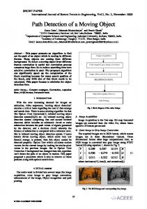
1.1. General Review Throughout the world, the detection was one of the first needed issues. Humans and animals are using it as a basic sense in their life. Today and during the development that happens in the revolution of technology, most of the things in our life are to be modeled and used industrially. One of these things is the detection technique, which represents the sense of sight. The high level devices like robots depend on detection essentially to do their work. Most of the important fields such as medicine, military, industry, security are used detection as an important thing of their work. In many applications those have to do tracking, the detection is needed as a basic operation. The need of detection is increased rapidly. Generally, the detection include two types (see Figure 1), it can be done by electronic components (like sensors), or image processing techniques.
(a)
Inductive proximity sensor
(b) Camera used in detection
Figure 1: Detection types in industrial line application (conveyer belt) 1
The first mentioned type of detection is used in instrumentation measurements, for examples: temperature, fire, and gas sensors, distance sensors measurements, electric, magnetic fields detection sensors, light and sunlight sensors, and ext. Hereby, this type handles with physical signals. The other type depends on using camera as sensor, this camera detects objects by images or videos capturing, this type of detection is using generally in surveillance systems. According to the application, the detection can be real time like industries, securities, and traffics applications, in others, the detection not needs to satisfy the real time, like medical, chemical and biological applications. The last mentioned detection technique is classified as an image processing technique, which is used today widely in most of the fields. The image processing detection techniques can be classified according to the detected regions (objects) into two types, moving and non-moving objects detection. Each of these two types has many standard methods, but sometimes a combination between two or many of these methods can be done obtaining more accurate results with lowest processing time. In this thesis, seven different detection methods are used, five of them are previously presented and used by others, the sixth method is the edges detection method (five types of edges detection techniques are used). The last one (method 7) is presented here, this method is proposed using a combination between method 5 and the canny edges detection type in method 6. All of the mentioned methods are applied for the same moving objects on the same application and under the same environment (the same place, time, light, and ext.). The obtained results are compared firstly depended on their consuming time. According to this comparison three types of these used methods (method 1, method 2, method 4) are neglected during to their high consuming time instead of its good quality in detection, the other four methods are then compared according to their detection accuracy. In the next step a detection accuracy comparison is done, the misclassification ratio is used to complete this issue. The used comparisons showed that many of the used method are doing well in detection but with high consumer time (method 1, method 2), in other type, some problems are happened in detection but with low consuming time (method 3), while in method 4 both of the detection errors and consuming time are high. Method 6 and method 5 are some degree well in detection with a low 2
consuming time. The obtained results proved that the presented method (method 7) which is combined between method 5 and method 6 is the best one according to its detection accuracy and consuming time. This presented method is finally used in the implementation of our application industrial line.
1.2. Thesis Organization Generally the image processing technique represented with its detection field is the main issue used in our thesis. It is used here for an industrial line application '' a prototype conveyer belt with a robot arm are work together depending on signals come from a single stationary camera mounted on the top of the conveyer belt". The details of this thesis's work are explained in the next chapters.
In chapter 2, a background theory for image processing detection methods, and the Robot kinematics with their details are explained. In chapter 3, a literature review for the related works is discussed with the advantages and disadvantages.
Chapter 4 involves the algorithms those used in our thesis, some of them are depended generally on the works of other researcher (the first five algorithms), these algorithms are used firstly without changes, and then some of them are improved to be more suitable to for our application. The edges detection techniques are used in the sixth algorithm and the proposed method's algorithm (method 7) is presented finally.
In Chapter 5, the descriptions of the used application (the designed conveyer belt and the used robot arm) are explained. The results with their figures and tables for the seven used methods are compared according to their consuming time and detection accuracy. Finally, chapter 6 included a conclusion of our thesis and the suggested future works are mentioned.
3
CHAPTER 2
BACKGROUND THEORY
2.1. Detections Techniques in Image Processing All of the applications those depend on the real surveillance video, have different needs, thus, most of them are required different treatment. The most important issue in these application systems is the detection operation, while the majority detected things are the moving objects. The Detection regions operations those correspond to moving objects such as people, vehicles, in outdoor environments, or the others in the indoor environment like the industrial line system in companies such as the conveyer belt [1], are the first basic step in any vision system, this detection operation can help the other subsequent analysis steps to complete all the system work. The detection processes of objects in the two dimensional images take place in many active applications. Many daily applications are used the detection, the medicine field, traffic supervision, access control, and in the identification and authentication systems [2]. The most related fields use the detection, are the industries those used the intelligent robots, which are indoor applications. Due to the mostly indoor problems of the sudden dynamic changes such as illumination, reflections, unstable lighting, unexpected motions, orientation, speed changes, the motion detection considered as a difficult problem to process.
2.1.1. Moving Object Detection The major moving objects detection methods are:
4
2.1.1.1. Temporal Differencing (TD) The temporal differencing attempts to detect the moving object by using the pixel by pixel difference of constructive frames (three or two frame at least) in video sequence (see Figure 2). The advantage of using this method of detection that it has a high degree of adaptation to the dynamic changes. The disadvantages of using it are the failing in detection of the whole relevant pixels for some types of moving objects. Also it fails to detect the stopped objects, thus, it is best to combine additional methods with it to make it more suitable for the detection of the stopped objects for the success of higher level processing.
Figure 2: Temporal differencing detection method 2.1.1.2. Background Subtraction (BS) The background subtraction is the common used technique for motion segmentation [3-4]. This technique attempts to detect the moving regions (moving objects) by subtract the current image (first video frame) pixel-by-pixel from the background image which is created by the images averaging technique (see Figure 3), during the initialization period.
Figure 3: Averaging operation for background modeling Using this technique depends on the threshold value of this operation, thus the pixels where the difference is above the threshold are classified as a foreground [5-6], while the other pixels are neglected and used as a part of background region, which is uploaded with the next images over the time to notice the dynamic changes on them. 5
This is the basic scheme of the background subtraction in terms of foreground region detection, which has many different approaches, background maintenance and post Processing. The advantage of using the BS is that of its well performing in extraction for most of the moving objects relevant pixels, even when they stop. It is the commonly used method in detection due to its ease of use and implementation. The disadvantages of using the BS is that it is usually sensitive to the dynamic changes for instance, the stationary objects are uncovered the background illumination or the sudden brightness. Heikkila and Silven in [7], are used the simplest version of this scheme where a pixel at location (
) in the current image
(first used frame of video) if the following equation is satisfied: | (
)
(
Where T is the predefined threshold, while
)|
(2.1)
which represent the background is
updated by using the Infinite Impulse Response according to the following equation: + (1 - α)
(2.2)
The creation of the foreground pixel map is mostly followed by the morphological closing to eliminate the small size unwanted regions. The BS method is mostly complete the feature data for the moving objects [6-7], it can be used firstly to detect the objects and then recognizing them depending on its features (see Figure 4).
Figure 4: Background subtraction detection method 2.1.1.3. Optical Flow The analysis of the images sequences are used to approximate motion , when the 3-D velocity vector of objects are projected into the image plane, that is known as the image flow field. If it is supposed that we are working in a reverse direction and get sequence of image (video frames) to determine the movement of objects that is leads approximately to the optical flow method [8]. Thus, the optical flow methods are depend on use of the flow vectors of moving objects over the time to detect the moving regions (objects) in images or video 6
frames. It can detect motion in video sequences even from moving camera. That is the significant issue of using the optical flow method than others. In [8], peter O'donovan explain the optical flow constraint equation, he mentioned that the most basic assumption made in optical flow calculations is the constancy of image brightness. It is simply assumption that when the changing position of object during a short interval t1 to t2 , the reflection and the illumination of that will not changes and remain constant. ( Where
(
)
(
) is the intensity of the image at position(
are the changes in position, while
)
(2.3) ), at time, and
,
is the change in time.
After applying the Taylor series expansion and ignore the higher order terms according to that of dealing with a small neighborhood, the equation will be according the following: (2.4) Where the equation I
=(
) is the spatial gradient, v = (
)
(
) is
optical flow vector and It is the temporal gradient. Because of the deals with the single displacements between two frames, this displacement which is equal to 1 (Δt=1) is not appears. It is important to say that the optical flow vector (
) is the
important issue to be mentioned here. There are many methods used to calculate the optical flow. In [9] there are many methods used to calculates the optical flow, such as differential methods (which is also contains types like Horn and Schunk and the Lucas and Kanade) and correlation based methods (Barnard and Thompson). Optical flow method is used mostly for the rotation motion of objects, also used for translation motion, but most of the time the optical flow method is very complex computationally and cannot be used in real time applications without a specialized hardware which will lead to an incremental of system price [10], thus it is not suitable to use for those applications which can be completed by using other methods more easier than the optical flow. The optical flow detection method has no responding to the stopped objects or those moving objects if a suddenly stop is happened [6-7-8]. 7
2.1.1.4. Statistical Method Most of the advanced methods those use the statistical characteristics of individual pixels are developed to overcome the shortcomings of basic background subtraction methods.
The statistical method is mainly inspired by the background subtraction method in the term of keeping and dynamically updating statistics of the pixels that belong to the process the background image.
The foreground pixels are identified by comparing each in frames with background model pixels. This approach has become the more popular one due to the reliability of containing noise scenes and other sudden changes on them [10]. According to [11], the system that named (W4) uses the statistical background model where each pixel is represented with its minimum and maximum intensity value (S,R), and maximum intensity difference (D) between any of the consecutive frames that observed during the initial training period where the images scenes of the video contains no moving objects. A pixel in the current image (first used video frame) is to be classified as foreground if it satisfies the following equation: | (
)
(
)|> (
) Or | (
)
(
)|
(
)
(2.5)
After determining the threshold value, a simple addition of morphological erosion can be applied to the detected pixels (foreground pixels), this additional iteration is applied to remove the noisy pixels. After that, a sequence of erosion and dilation are used for the foreground map. The purpose of doing that is to grow the eroded regions to their original sizes. In order to find the region of interest, small-sized regions are to be eliminating after applying connected component labeling. Over the time, the new images data are used to update the statistical of background pixels those represent the non-moving objects (regions) of current image. The statistical method needs many training samples and also has much computational complexity; because of that, it is mostly not used for real time applications.
8
2.1.2. Feature Detection (Computer Vision) Features are used as the starting point for many computer vision algorithms, most of the time; algorithms are classify as good algorithms or not according to their features detectors. The feature detection is the low level of the image processing operation, it is really the first operation performed in the images. By using it, every pixel inside the image will be examined, sometime, only the region of features in the images can be examined. Sometimes, when the features detection has complex computations and need a long time to complete, a higher level algorithm may be used to guide the feature detection stage, so only a part of the image (region of interest) will be searched for the features. Today many computer vision algorithms use the features detection as an initial step; as a result, many hundreds of feature detectors are developed. These developments are varied widely according to the detected features, these features detectors can be classified according to the following sections: -
2.1.2.1. Edges Feature Detection The edges feature detection is a process that detects the presence and location of edges, modeled by sharp changes in color intensity (or brightness) in images. It can be confirmed that the discontinuities in image brightness are probably matched to discontinuities in depth, in surface orientation, sudden changes in the properties of material and differences in the illumination's scene. An important property of the edge detection method is the ability of it to extract the accurate edge line with well orientation. There are many type of Edge feature Detection, the most used edges methods are: Canny, Differential(Laplace), Sobel, Prewitt, Roberts and ext.
2.1.2.2. Corners Feature Detection The Corners are points in images that have a local two dimensional structure. The Corners detection is emerged during the beginning of the algorithms performing of 9
the edge detection, and then edges are analyzed to find the rapid changes in direction. These algorithms were then developed to make the explicitly of the edges detection is no longer required, immediately by looking for high levels of curvature in the gradient of image. Then, it is noticed that the corners were being detected also on the parts of images which were not corners in the traditional concept. These corners (detected points) are usually known as points of interest, but normally the 'corner' is used. The mostly used algorithms for corners detection are: Harris operator, Shi and Tomasi technique, Level curve curvature, and SUSAN corner detection method.
2.1.2.3. Blobs (Region of Interest) The Blobs provide an integrated description of image structures in terms of regions, unlike corners that are many of the corners are similar. The blob descriptors mostly contain a preferred point which means that many blob detectors can also be regarded as operators of interest point. The blob detectors able to detect areas in too smooth images which are not easy to be detected by corner detectors. When reduction is considered in an image and the corner detection are to be performed. Then the detector will respond to the points which are sharp in the reduced image, but that may be lead to a smooth in the original image. At this point the difference between the corner detector and the blob detector becomes rather opaque. Usually, this identification can be redressed by including an occasion concept of scale. The mostly use Blobs algorithms are: Laplacian of Gaussian and the Difference of Gaussian.
2.1.2.4 Ridge Sets Feature Detection The ridges sets are representing very important geometric information intrinsic to a function. The initial motivation for the ridge detection creation has come from the computer vision and image analysis that is to capture the internal longitude objects in the image. The Ridge representations in terms of turning points have used for image segmentation. These representations have been attempts to capture the objects' shapes using graphical based representations that can reflect the ridges. These representations can be sensitive to the noise if they computed at only one scale, 11
representation of objects (or shapes) in the image. The most used Ridges algorithms are the Hough transforms and Structure tensor.
2.1.3. Morphological Operation in Detection Inside the mentioned methods before, there are many other type methods used in image processing detection, one of these methods is the morphological operations. Generally, it is a theory of analyzing and processing of geometric structures, applied mostly for digital images to extract the components from the image's objects [12]. It is mostly used to select the object according to their shape and regions, to do that a suitable structure element have to be used in order to complete the work successfully. There are many available structure elements such as: ball, square, disk, line, and triangle. There are many morphological operations types, these are erosion, dilation, opening and closing. The morphological operations are usually applied for the binary images. Which are essentially came from converting the colored images. In binary images the white pixels are normally used for the foreground regions, while the black pixels are used for the background regions, in many implementations this convention is reversed [13]. The erosion operation is one of the basic morphological operations in the area of mathematical morphology; some visions of it can be applied for the gray images. This operation is used to erode a way of the region's boundaries for the foreground pixels. Because of that, the foreground pixels' area has to shrink in size, while the holes within this area become larger [13]. The dilation operation is the second basic morphological operations in the area of the mathematical morphology, as the erosion, it is usually used for the binary images, but in many versions, it can be used for the gray. This operation is usually used the structure element to probe and expand the object's shape [13]. The opening and the closing operations include using the erosion and the dilation together, one after the other. In the opening operation the erosion is applied and then followed by the dilation, while in closing operation the dilation is followed by the erosion.
11
The morphological operations can be used in detection inside other detection methods or feature detection, it can be used individually in many applications. Usually the morphological operation are used when the area, size number of pixels are needed as features of recognition, but it is not suitable to use when the color or texture are to be considered in recognition [12-13]. 2.2. Robot Kinematics In any robotics study, it is constantly concerned with the location of objects in threedimensional space. These are the links of manipulator, the parts and tools with which it deals, and the manipulator's environment. Generally, they are described by only two attributes: position and orientation [14]. Naturally, only one topic of immediate interest is the manner in which we present the quantities and manipulate them mathematically. In order to describe the position and orientation of a body in space, we will always attach a coordinate system, or frame, rigidly to the object. We then proceed to describe the position and orientation of this frame with respect to some reference coordinate system. Any frame can be served as a reference system within which to express the position and the orientation of a body, so we often think of transforming or changing description of these attributes of a body from one frame to another [15]. 2.2.1. Description of Robot Arm The (Lynx6) robot arm has five degree of freedom of motion (DOF) inside a rig movement, it is similar to the human arm according to the number of joints point of view [15]. These joints provide shoulder rotation, shoulder back and forth motion, elbow motion ,wrist up and down motion, wrist rotation and gripper motion (Figure 5).
12
Figure 5: Lynx 6 robotic arm
Joint 1 represents the base, its axis is z0; Joint 1 provides the Ѳ1 rotational angular motion around z0 axis in x0y0 plane.
Joint 2 is identified as shoulder; its axis is perpendicular to joint 1 axis. Joint 2 provides an angular motion Ѳ2 in x1z1 plane.
The z axes of Joint 3 (Elbow) and Joint 4 (Wrist) are parallel to the z-axis of joint 2. They provide Ѳ3 and Ѳ4 angular motions in x2y2 planes respectively.
Joint 5 is identified as a gripper. The z-axis of Joint 5 is vertical to z-axis of Joint 4; Joint 5 provides Ѳ5 angular motion in x4y4 plane [15]. A graphical view of all the joints was displayed in Figure 6.
Figure 6: Coordinate frames of L6 robotic arm
2.2.2. Servo Controller Card The (Lynx-6) Robot Arm rotational joints and its gripper are controlled by dedicated servo motors. These motors are connected to a serial servo controller card (SSC32) to control the (Lynx-6) from a computer through the serial port, Fig. 7. A sequence of three consecutive unsigned bytes is sent to a serial servo controller from the computer. These are the default sync byte, the joint servo identifier byte and the 13
desired position byte. Rotational position of a servo motor is determined by specific angle, this angle value that is provided by the computer was digitized to generate discrete motional steps by SSC-32 card [16].
The SSC-32 servo controller card provides the hardware interface between the computer and the robot arm. It has a time resolution of (1 μs) for accurate positioning and a dc motor control to generate extremely smooth moves. The time range is 0.50 msec. to 2.50 msec. for an angular range of 0o to 180o. The card generated motion can be a speed controlled, time controlled or combination motion (speed and time) [16].
Figure 7: SSC-32 servo controller card
2.2.3. Forward Kinematics Kinematics is the science of motion that treats motion without regard to the forces which cause it. Within the science of kinematics, one studies position, velocity, acceleration, and all higher order derivatives of the position variables (with respect to time or any other variable(s)). Hence, the study of the kinematics of manipulators refers to all the geometrical and time-based properties of the motion. The manipulators consist of nearly rigid links, which are connected by joints that allow relative motion of neighboring links. These joints are usually instrumented with position sensors, which allow the relative position of neighboring links to be measured. In the case of rotary or revolute joints, these displacements are called joint angles. The number of degrees of freedom that a 14
manipulator possesses is the number of independent position variables that would have to be specified in order to locate all parts of the mechanism. This is the general term used for any mechanism [17].
Robot kinematics refers the analytical study of motion of a robot manipulator. Denavent-Hartenberg (D-H) method that uses four parameters is the most common used method for describing the robot kinematics. These parameters ai-1, αi-1, di and θi are the link length, link twist, link offset and joint angles respectively. The coordinate frame is attached to each joint to determine D-H parameters. Zi axis of coordinate frame is pointing along the rotary direction of the joint. The transformation from joint i to joint i+1 is obtained by the matrix transformation [17].
(2.6)
D-H parameters for (Lynx-6) are defined for the assigned frames in Table 1. For example Frame five is the grip frame with attached end effectors at joint five (see Fig. 6). Table 1: DH Parameters for Lynx 6 Robotic Arm Frame
αi-1
ai-1
di
θi-1
1
0
0
b
θ1
2
90
0
0
θ2
3
0
L1
0
θ3
4
0
L2
0
90+θ4
5
90
0
d5
θ5
By substituting these parameters; the transformation matrices T1 to T5 can be obtained as shown below. For example, T1 shows the transformation between frames 0 and 1 (designating ci as cosθi and si as sinθi, etc). 15
c1 s T1 1 0 0 c 4 s T4 4 0 0
s1 0 0 c 2 0 c1 0 0 T2 s2 0 1 b 0 0 1 0 s4 c4 0 0
s2 0
0 0 c 3 s 1 0 T3 3 0 0 0 0 1 0
c2 0
0 L2 c 5 0 0 0 T5 s5 1 0 0 1 0
s5 0 c5 0
0 0 1 d 5 0 0 0 1
s3 c3 0 0
0 L1 0 0 1 0 0 1
(2.7)
(2.8)
Calculating the position and orientation of the end effectors with given joint angles is called Forward Kinematics analysis. Forward Kinematics equations are generated from the transformation matrixes shown below and the forward kinematics solution of the arm is the product of these five matrices identified as Tg (with respect to base). The first three columns in this matrix represent the orientation of the end effector, whereas the last column represents the position of the end effector [17]. The orientation and position of the end effector can be calculated in terms of joint angles.
nx n Tg T1 T2 T3 T4 T5 y nz 0
ox oy
ax ay
oz 0
az 0
px p y pz 1
(2.9)
nx= – c1 c5 s234 + s1 s5
(2.10)
ny= – s1 c5 s234 – c1 s5
(2.11)
nz= c5 c234
(2.12)
ox= c1 s5 s234 + s1 c5
(2.13)
oy= s1 s5 s234 – c1 c5
(2.14)
oz= – s5 s234
(2.15)
ax= c1 c234
(2.16)
ay= s1 c234
(2.17) 16
az= s234
(2.18)
px= c1 (d5 c234 + L2 c23+ L1 c2)
(2.19)
py= s1 (d5 s234 + L2 c23+ L1 c2)
(2.20)
pz= d5 s234 + L2 s23 + L1 s2 + b
(2.21)
2.2.4. Inverse Kinematics The inverse kinematic analysis determines the joint angles for desired position and orientation in Cartesian space. The solution is much more complex than direct kinematics since there is no unique analytical solution. Each manipulator needs a particular method considering the system structure and restrictions [18]. In the solution, the user specifies the desired target position of the gripper in Cartesian space as (xd, yd, zd). The lengths b, L1, L2 and d5 correspond to the base height, upper arm length, forearm length and gripper length, respectively. The angles θ1, θ2, θ3, θ4 and θ5 correspond to shoulder rotation, upper arm, and forearm, wrist, and end- effector, respectively. These angles are updated as the specified position in space changes. Here we focus on the inverse kinematics for the wrist without taking the gripper into the account. Considering the wrist without taking the gripper into account means that the robot arm can be described as a 2R planar manipulator on a rotating base.
2.2.4.1. Base Joint Angle The user specifies the desired target position of the gripper in Cartesian space as (xd, yd, zd) where zd is the height, and (ϕ) the angle of the gripper relative to ground [1814]. In addition, by either keeping ϕ fixed in position mode or keeping the wrist fixed relative to the rest of the arm, the inverse kinematic equations can be solved in closed form as show now for the case of the fixed ϕ. The Solving of the base joint angle according to Fig. 8, gives:
√
(2.22) 17
cos (Ѳ1)
(2.23)
yd= d sin(Ѳ1)
(2.24)
1 A tan 2 ( y d , x d )
(2.25)
d=d
yo yd
d θ1 O xd
xo
Figure 8: Lynx-6 base angle
Z for Arms 2.2.5. Algebraic Solution d5 4 Consider the three-link planar manipulator and using DHθparameters, we can use the
z'
θ3 link parameters easily to find the kinematic equations of this arm: L2
C234 S 234 B 2 Sθ234 C234 W T 4T 02 0 0 0 O L1
0 0 1 0
L1C2 L2C23 L1S 2 L2 S 23 0 1 D
(2.26)
d
To focus our discussion on inverse kinematics, we will assume that the necessary transformations have been performed so that the goal point is a specification of the wrist frame relative to the base frame, that is
Because we are working with a
planar manipulator, specification of these goal points can be accomplished most easily by specifying three numbers: xd, zd, and ɸ where ɸ is the orientation of link 3 in the plane (relative to the + ̂ axis). Hence, rather than giving a general
as a
goal specification, we will assume a transformation with the structure:
18
C S 2 4T 0 0
S C 0 0
0 xd 0 z 1 0 0 1
(2.27)
Where z zd b
(2.28)
All attainable goals must lie in the subspace implied by the structure of equation (2.33). By equating (2.26) and (2.27), we arrive at a set of four nonlinear equations that must be solved for θ2, θ3 and θ4:
C C 234
(2.29)
S S 234
(2.30)
x d L1C 2 L2 C 23
(2.31)
z L1 S 2 L2 S 23
(2.32)
We now begin our algebraic solution of equations (2.29) through (2.30). If we square both (2.31) and (2.32) and add them, we obtain:
xd2 z 2 L12 L22 2 L1 L2C3
(2.33)
Where we have made use of C23 = C2C3 – S2S3
(2.34)
S23 = C2S3 + S2C3
(2.35)
Solving (2.23) for c3, we obtain
C3 xd2 z 2 L12 L22 /( 2 L1 L2 )
(2.36)
In order to do a solution to exist, the right-hand side of (2.36) must have a value between -1 and 1. Physically, if this constraint is not satisfied, the goal point will be too far to reach the manipulator. If the goal is in the workspace, the expression can be written according to the following S3equation: S 3 1 C32
(2.37)
Finally, compute θ3 using the two-argument arctangent routine: 19
θ3 = A tan2 (S3, C3).
(2.38)
The choice of signs in (2.37) corresponds to multiple solutions in which it can be chosen the "elbow-up" or the "elbow-down" solution. In determining θ3, It is possible to use one of the recurring methods for solving the type of kinematic relationships that often arise, namely, to determine both the sine and cosine of the desired joint angle and then apply the two-argument arctangent. That make us sure that we have found all solutions and that the solved angle is in the proper quadrant to found θ3, it is possible to solve (2.32) and (2.31) for θ2. It can be written in the form: xd= k1C2 – k2S2
(2.39)
z'= k1S2 – k2C2
(2.40)
k1= L1 + L2C3,
(2.41)
k2= L2S3
(2.42)
Where
In order to solve an equation of this form, it can be perform a change of variables. Actually, it is changing the way in which it is possible to write the constants k1 and k2. If r =+√
(2.43)
γ = Atan2 (k2, k1)
(2.44)
k1 = r cos γ
(2.45)
k2 = r sin γ.
(2.46)
And
Then
Equations (2.43) and (2.45) can now be written as:
xd cos cos 2 sin sin 2 r
(2.47)
21
z cos sin 2 sin cos 2 r
(2.48)
So cos 2
xd r
(2.49)
sin 2
z r
(2.50)
Using the two-argument arctangent, we get
z x 2 A tan 2 , d A tan 2 ( z, xd ) r r
(2.51)
θ2 = Atan2(z', xd) – Atan2 (k2, k1)
(2.52)
And so
Note that, when a choice of sign is made in the solution of θ3above, it will cause a sign change in k2, thus affecting θ2. The substitutions used, (2.43) and (2.45) constitute a method of solution of a form appearing frequently in kinematics namely, that of (2.31) or (2.32). Note also that, if xd = z' = 0, then (2.52) becomes undefined - in this case, θ2 is arbitrary. Finally, from (2.29) and (2.30), we can solve for the sum of θ2through θ4: θ2+ θ3 +θ4 = Atan2 (Sɸ, Cɸ) = ɸ.
(2.53)
From this, we can solve for θ4, because we obtained previously angles θ2 and θ3.
21
CHAPTER 3
LITERATURE WORK REVIEW
3.1. Introduction Since many years ago, the researchers work in the fields of detection which is a branch of the image processing techniques, many methods are discovered, many others are improved, especially the moving objects detection methods, which are being very important for many fields today. In this chapter, many of the previews related work will be mentioned, with their descriptions, details, advantages and disadvantages. These acknowledgments help us to select the best method, with lowest cost, and given the best results to be used in our work.
3.2. Previews Related Work The motion detection refers to the capability of any surveillance system to detect the motion and recognize the changes. Without use of a specific detection method, it is not possible to build a good surveillance system [19]. In the following, many types of detection methods used and presented by researcher which are related to the work that we have to do.
3.2.1. Moving Object Detection Using Rigidity Constraint In [3] William B., et.al describe a method for visually detecting moving objects from a moving camera constant to movement of the objects correspondences in two orthographic views. They present an alternate approach based on the rigidity constraint. A scene containing moving objects can be thought of as undergoing a particular
sort
of
non-rigid
motion
with
respect
to
the
camera. 22
The Structure-from-motion techniques that are sensitive to the presence of such nonrigid motions can thus be used to detect moving objects. They use the linear structure-from-motion (SFM) algorithm to solve for partial parameters governing the relative motion of camera and background. This method is demonstrated on real image sequences for which point correspondences have been determined in a fully automated manner. They adopt the convention that the coordinate system is fixed to the camera; therefore, the camera's motion is equivalent to the environment that contains moving regions by a stationary camera. The researchers go on to develop a solution by using the two-view case to determine constraints on object rotation between each pair of images in the threeview situation and then find the unique motion making these constraints consistent. The work depends on the applying the rotation and translations equations over the objects coordinates space for the object inside image. The method supposes that the camera is moved with the same speed and direction with the object, it depends on two coordinates to detect objects with three coordinates. The used method is good for detection inside involving tracking depends on the objects-camera moved at instance.
3.2.2. Background Subtraction for Moving Object Detection The background subtraction method is used widely. Dinesh Nair, et.al, present a system that detects unexpected moving obstacles that appear in the path of a navigating robot, and estimates the relative motion of the object with respect to the robot [20]. The system is designed for a robot navigating in a structured environment with a single wide-angle camera. The objective of the system is to detect moving obstacles in order to gradually stop the robot to avoid collision. The system uses polar mapping to simplify the segmentation of the moving object from the background. The polar mapping is performed with the focus of expansion as the center. The detecting moving objects from a moving platform using only a vision sensor (camera) use temporal or spatial disparities estimated from the image sequence for detection purposes. To segment moving objects from the background, each image acquired by the robot is transformed from Cartesian coordinates to polar coordinates, 23
using a polar mapping that transforms the image to a polar coordinate system with the focus of expansion as the center. The used method not includes information about the object size, dimensions, and features. The advantage of this system is to realize the task of moving obstacle detection from the robot with the aim of a real-time effective implementation.
3.2.3. Morphological Operation Used for Moving Object Detection The use of morphological operation for object detection is depended basically on their pixels (foreground region in pixels), the opening, closing (erosion, dilation) are used to select the object of interest according to a threshold value used to do this issue. In [21] Foresti G., Present a visual surveillance system for remote monitoring of unattended outdoor environments. The system, which works in real time, is able to detect, localize, track, and classify multiple objects moving in a surveilled area. The object classification task is based on a statistical morphological operator, the statistical pecstrum (called spectrum), which is invariant to translations, rotations, and scale variations, and it is robust to noise. In particular, it involves the real-time analysis and description of complex scenes (also containing object occlusions) from image sequences. Performances about good classification percentage, false and missed alarms, viewpoint invariance, noise robustness, and processing time are evaluated. The classifications here is done for vehicles like cars Lorries and other types, this classifications is done depending on the size (area in pixels) for each object (vehicle) The morphological opening operation (erosion and dilation) is used to do the classification according to the area that calculated depending on the element used for this operation (disk, square, ext.). The railway is used here to test the system, they assumed that the vehicle is go across the rail and at the time we can detect the moved object (vehicle) to avoid any collision may be happen, for example. If the area that detected by the opening operation is more big, we can assume that more than two vehicle is at the rail, may be an accident happened and then the rail will be stopped. According to the author, this system is more suitable for both real time surveillance and for monitoring system. Real-time object recognition is the main novelty of the 24
paper. In this work the camera is stationary and on the top high point to recognize any moved objects. The image that gotten from video after applied the opening will be mostly black (background) and the other part appeared with its motion clearly. A background updating module is devoted to estimate significant scene modifications due to illumination changes or entrance of new objects. Then, the minimum bounding rectangle (MBR) of each detected image blob is computed.
3.2.4. Background Subtraction Combined with Temporal Differencing Detection Methods As mentioned before, the background subtraction is the mostly used method in detection, as other methods; it has many disadvantages during to its use. Because of its high sensitivity to the sudden illumination and brightness changes [3-4], the background subtraction is usually supported using other type of detection method. In [13] Guanglun L, and et.al., presented a method for real-time moving object detection. The method assumes that the foreground is segmented by both background subtraction and temporal differencing methods. According to the researchers, the experimental results demonstrate that the proposed method can update the background exactly and quickly along with the variation of illumination, and the moving objects can be extracted effectively. The background will be updated here continually. In order to overcome the impact of changes in the environment and raise the degree of automation, the adaptive threshold has also adopted. This method is not only robust to the noise impact, but also to reduce the tiny objects or unwanted parts. This approach builds fast adaptive background models that reduce the sensitivity towards the illumination changes [22]. With this approach, it is possible to detect new objects in the scene even if they suddenly stop moving. It is also possible to detect objects that have removed from the scene. The AND OR operators are applied to the images (two images) and in order to cope with sudden light changes and leaves swings situation. The morphological operations are used to eliminate the unwanted part depending on the used threshold values.
25
3.2.5. Background and Foreground Modeling Method for Detection Method In most of the detection method, one of the background or foreground has to be modeled using a suitable detection method, most of the time the modeling is used for the foreground region (the object that needed to be detected), many time during the detection operation, a region of the image background selected as a part of foreground, that happens because of the noise or other sudden changes. In [23] C. Cuevas, et.al., presented a novel and fast strategy for moving object detection by non-parametric background- foreground modeling is proposed. The background is modeled using only color information; while both color and space are considered for the foreground modeling. High-quality segmentation results are obtained while the computational cost is dramatically reduced. In this approach the spatial information is considered only for the foreground modeling lead to greatly decreased computational cost in the background modeling. Both the background and the foreground models are combined using a novel Bayesian approach. By an iterative multi-tracking strategy, the coordinates of the foreground data are updated from each image to the next. The foreground displacements between consecutive images are obtained recursively. For the combination of background and foreground likelihoods, they have modeled both foreground and background. The background is modeled by exclusively using color information, the foreground modeling considers both spatial and color. The application of an efficient iterative multi-tracking algorithm allows updating the previously detected foreground information and improving the foreground modeling. Both the background and the foreground models enable an important reduction of several orders of magnitude in computational requirements.
3.2.6. Harries Corner Detection with Masking Operation Used for Moving Object In [24] Albiol A. and et.al., try to solve problems happens in urban traffic which are currently real problems for most medium-sized and large cities. To reduce the problems caused by traffic congestion, intelligent transportation systems (ITS) are being deployed worldwide to achieve a more efficient use of existing infrastructures. They used a special methods to detect stationary objects which is here represented by 26
the stopped vehicles (stopped cars), they mentioned many works before those used the background subtraction and also foreground, they compare the current cases with the both foreground and background, and for those objects (stopped vehicles) for a long time are similar to the background. These cars classified as a background while those with the short time stopping classified as a foreground. In this work a single stationary camera is used to monitor the road from a high building, and then the background is initialized. The low level feature points (Harries corners or Shi Tomassi) are used then to detect the objects without performs any type of objects. The mask operation is used then to select the region of interest to detect the stopped cars in the second line of the road. To do that successfully the morphological operations is used to eliminate the corners of the not wanted detected parts like the white lines in the roads. After that the detected corners are classified according to the detected objects, the dynamic parts and the static parts. That is done by compare the corners values with a thresholds, if the values is more than the thresholds that lead to classify the corners as a dynamic type, if not the corners will be classified as a static type. These steps are repeated for every video frame and the founded values are to be updated for every day.
3.2.7. Multilayer Codebook-Based on Background Subtraction Used for Moving Object Detection In [25] Jing-Ming Guo, et.al., are presented a multilayer codebook-based background subtraction (MCBS) model which is proposed for video sequences to detect moving objects. A
Combining of the multilayer block-based strategy and the adaptive
feature extraction from blocks of various sizes is done. By using this method most of the non-stationary (dynamic) background can be removed and the processing efficiency is significantly increased. The pixel-based classification is adopted for refining the results from the block-based background subtraction, which can further classify pixels as foreground, shadows, and highlights. The proposed scheme can provide a high precision and efficient processing speed to meet the requirements of real-time moving object detection.
27
The disadvantages for using this method is that because the MCBS employed RGB information for modeling the background subtraction, it was difficult to distinguish the foreground and background when they have similar colors.
3.2.8. SIFT Harries Detector in Hashed Image Used for Object Detection In many environments (indoor or outdoor) the detection is done depended only on images captures by camera. That can be used especially in applications those not need tracking. When the researcher depend on one or many captured image only, the user can obtain more flexibility in choose the suitable method and get a good results. The hashing image technique which is used to reach the feature and detect it more easily, is used for detection in images or video frames, but not possible to use it when the real time is needed in displaying the video. Many applications are really needed real time in their work, but not exactly in video displaying, these applications can use the image hashing techniques for detection purpose. In [26], Xudong L. and et.al., used hashing images that is used in secured detection systems generally. The SIFT-Harris detector is applied then for each part of the hashed image; they applied the method for many types of distorted images, like noise, compression, blurring, geometric attacks such as rotation attacks and brightness, inside many other causes. These methods can be used for the image enhancement applications, it is not suitable for real time application displaying videos, without additional hardware, but it is better for complex features images, secured information inside images, water marking, and ext. 3.2.9. Adaptive Background Generation Using Special Camera Some type of detection methods depend on adding some type of hardware usage or a special type of cameras. In [27], Seungwon L. and et.al., presented a method for adaptive background generation for automatic detection of initial object region using multiple color-filter aperture camera-based surveillance system. This method is used to realize simultaneous object detection and depth estimation using multiple colorfilter apertures camera. The detection operation that used by this camera is done depending on using the optical flow detection method. 28
The researchers presented a novel color-based background generation method which can reduce the interference in the object region for stable depth estimation. For efficient estimation of color shifting vectors in the extracted object region, a simplified elastic registration (ER) algorithm is used. The object distance is determined by using the relationship between the pre-specified distance transformation function and the estimated shifting vectors of the corresponding object region. The object detection method that used the adaptive background generation for single camera-based is fully automatic object tracking and distance estimation. The object regions are detected using background subtraction between input and background images, while the background images are to be updated depending on any changes happen in the non-moved regions. Because RGB color planes of the detected object region are misaligned among each other, shifting vectors between green-and-red and green-and-blue channels are estimated by using the simplified elastic registration algorithm. The original elastic registration which is used here is the key factor to enable real-time depth estimation and tracking, which is the primary condition for consumer applications. Finally, the object distance is determined by using the relationship between the pre-specified distance transformation function and the estimated shifting vectors of the corresponding object region. According to mentioned descriptions of this work, any related adjacent work will be with the use of the used camera. 3.2.10. Edges Detection Techniques Edges detection technique is one of the most important tasks used in image processing field [27], it is used to detect the most complex features inside the images and video frames, this techniques has improved, many new types are added to their previews types, the most knower types are: Canny, Sobel, Laplace, Prewitt, and Roberts . These methods are different to each other on their basic mathematically work. The edges detection is used in most of the time inside other type of detection methods, essentially when related to the moving object detection. In [29] the edge detection is used to detect text inside videos, the operation is depended on the text color and the background contract of the video, the illumination changes and the 29
added noise can make a big problem for the detection here. In many other works the edges detection with their different types are used for the complex texture images and video frames, sometimes it is used to support other detection methods to solve their problems in detection [27]. The edges detection methods are different to each other in their work, the consuming time, the detection accuracy inside their basic mathematical and the complexity of their work. The mentioned methods (indoor and outdoor) those used before are suitable to use in our indoor application but different to each other in their proficiency, the qualification of using these methods depends on many basic factors adopted in our works to choose the best. These factors are assumed according to the application requirements. The processing consumer time, detection accuracy, real time achievement under the same environment's conditions, are the most important factors used to classify the detection method and select the best possible one to be adopted in our application. The used methods with their algorithms are described in details chapter 4.
31
CHAPTER 4
THE PROPOSED DETECTION METHODS
4.1. Introduction In this chapter many methods for detection will be mentioned, The proposed methods are selected from many reviewing works presented before, others general detection method are tested individually and then combined with some of the used method to achieve improvement and making them more specific to be use in our application and also more suitable to use in general .
4.2. Method of Working In this thesis, seven methods are used and compared one to each other. The first five methods are used from the literature works with some improvement added to them. The last two are the edges detection techniques (five types), and new method presented using a combination between two types of methods.
4.2.1. Method 1 (M1): Harris Corner Detection with Mask Operation (HCDMO) In this method [24], the Harris corner detection is used inside the masking operation to eliminate the not wanted regions in images and focus in the needed parts only, the used steps are as the following:
Read video and select the frame that include the object.
Apply the masking operation for the image to select the region in where the object can be reached in.
Convert the image into gray level 31
Apply the canny edge detection over the masked image
Apply the erosion and the dilation to eliminate the noisy points and get a clear image.
Apply the Harris corner detection to detect the object of interest.
Bounding the detected object and give the dimensions according to the detected corners.
4.2.2. Method 2 (M2): Image Hashing with SIFT-Harris Corner Detection This method is used the SIFT-Harris corner detection inside using the hashing techniques to find the interest features in limited parts of the images [26]. In this method the color is used as feature of interest in the SIFT-Harris inside using the hashing operation. The steps of detect one object using this type of detection is as the following:
Read video and convert it in frames.
Scaling the image to double and select the color used to be not detected as SIFT
Initializing the Hashing information
Opening two for loop to segment the images
Apply the SIFT-Harris for each block of the hashed image
Display the results
End the two loops
4.2.3. Method 3 (M3): Combining Background Subtraction and Temporal Differencing with MBR (BSTD with MBR) The method of using both background subtraction and temporal differencing is presented to get a more adaptive result than the results given by using one of the two methods individually [22]. In the following sections let's behave with the background subtraction firstly, then combine it with the temporal differencing and compare the results. This method is improved here by added the blobs MBR and also depends on
32
the binary mode of the detected images instead of the original RGB mode. The details are explained in the following sections.
4.2.3.1. Background Subtraction (BS) The most known problem in using the background subtraction is the high sensitivity to the sudden illumination and brightness changes in video frames and images. Sometime the sunlight, indoor light and the camera flasher in the objects classified as a part of background in other cases the shadows in the background regions classified as a part of the foreground region (the needed parts to be detected as foreground). The background subtraction can be used for the original image for the applications those behave with the images itself like the surveillance or monitoring application, in other type the detected images are used for other purpose like our application, in this type of detection the binary images can be used to reach the exactly region of interest with fewer number of false detected pixels. These two cases have algorithms as show in the following steps:
Case One: Apply the subtraction for the original images (object one used as a sample)
Get snapshots for the conveyer background before putting the objects
Calculate the background image using the averaging operation
Get new snapshot for the belt after putting the objects on it
Apply the background subtraction method for the current frame
Convert the image into gray mode
Apply median filter
Apply the erode operation
Display the results
Case Two: Apply the subtraction for the binary images (object one used as a sample):
Get snapshots for the conveyer background before putting the objects 33
Calculate the background image
Convert the background into binary mode
Get snapshot for the belt after putting the object inside the conveyer belt
Convert the object into binary
Apply the background subtraction
Apply median filter for the result
Display the result
4. 2.3.2. Background Subtraction and Temporal Differencing (BSTD) The background subtraction is usually used inside many other methods in detection. The corners detection and the edges detection and the blobs (region of interest) are usually used inside it, many other novel methods are presented by combining many types of detection together. In [22], the temporal differencing is combined with the background subtraction to make it more adaptive to the brightness and sudden illumination changes. As mentioned in the previous method (B.S), which is used here inside the use of the temporal differencing method, the detection can be applied for the original image and the binary image mode; the following cases algorithms explain the steps of these two cases:
Case One: (Apply the method for the original image)
Get snapshots for the conveyer background without the objects
Calculate the background image
Put the object inside the conveyer
Get snapshot for the object to be detected
Apply the background subtraction
Apply The temporal differencing method
Display the result
Merge the resulted images and find the average image
Apply median filter
Display the resulted images
34
Case Two: (Improve the used method by converting the result into binary mode)
Get snapshots for the conveyer background without the objects
Calculate the background image
Convert the background into binary mode
Put the object inside the conveyer
Get snapshot for the object to be detected
Convert the object into binary
Apply the background subtraction
Apply The temporal differencing method
Display the result
Merge the resulted images and find the average image
Apply median filter
Display the resulted image
4.2.4. Method 4 (M4): Background and Foreground Modeling Combination (BFMC) In this method the background region is modeled according to the color while the foreground modeled according to the color and the space [23], then combining the result. The algorithm for the presented method has the following steps:
Get many snapshots for the conveyer background without any objects
Put the objects inside the conveyer
Get many snapshots for the objects inside the conveyer
Modeling the background using the averaging image
Convert the results into binary level image
Inverse the image
Modeling the foreground image from the averaging image that is from the objects images
Convert the image into binary
Apply the dilation operation to eliminate the not wanted parts to be detected 35
Draw a rectangular around the object and get the centroid ,dimensions of the object
Combine the background and the foreground in one image
4.2.5. Method 5 (M5): Statistical Morphological Operation with MBR This method is used to detect objects, with its location, and classify multiple objects moving in a surveilled area in pixels. The classification of objects is done depending on the area of the detected objects, then the MBR to draw a rectangular around the detected area and gets the orientation, and the centroid of the detected region. The algorithm of using this method is as the following steps:
Get snapshots for the conveyer background after putting the objects inside it
Convert the image into gray mode
Convert the gray to binary image
Apply the morphological opening operation
Labeling the objects
Apply the average filter for noise reduction
Compare the foreground region with the wanted factor to be detected
If the object reach the factor
Apply the MBR to find the area , centroid , orientation , draw the bounding box
End if
Display the results
4.2.6. Method 6 (M6): Edges Detection Techniques One of the most used and important method used in detection is the edges detection techniques. There are many types of edges detection, five of the famous types are used here, Canny, Sobel, Laplace, Prewitt, and Roberts .Sometime these methods not used lonely, the algorithms of using this method has the following steps:
Get snapshots for the conveyer background with the objects
Convert the image into gray mod
Convert the gray image into binary mod 36
Apply the edges detection methods (one of the mentioned edges detection types for each time).
Display the results
4.2.7. Method 7 (M7): Statistical Morphological Operation with MBR and Edges Detection The Detection method which is in (4.2.5) is improved by adding the edges detection techniques in (4.2.6). The developed method is used to improve and enhance the results those come from using the methods in (4.2.5) and (4.2.6) to detect many objects those not detected using these methods individually.
Get snapshots for the conveyer background with the objects
Convert the image into gray mode
Apply Edges Detection Techniques (canny edges detection type)
Convert the gray image to binary image
Apply the morphological opening operation
Labeling the objects
Apply the average filter for noise reduction
Apply the MBR to find the area , centroid , orientation , draw the bounding box
Display the results
37
CHAPTER 5 EXPEREMENTATION RESULTS AND IMPLEMENTATIONS
5.1. Experimental Set Our industrial line application consists of a conveyer belt; a robot arm and a single stationary camera which is mounted on the top of the conveyer belt and connected to the PC (see Fig. 9). The mounted camera is used to detect the objects those moved through the conveyer belt, the captured video frames those include the detected objects will be processed using Matlab detection program. In our application, the real time must be satisfied in the detection operation inside the detection accuracy.
Figure 9: Application sets 38
In order to explain our application, we can suppose the following: many different objects are on the conveyer built, we need to detect one or many of these objects during its movement according to their features, then inform the robot arm which is in the other side of the conveyer to move the object to other location . (See Figure 10).
Figure 10: Moving object detection in an industrial application line
According to the obtained results, the robot arm will grip the object, if any error happened during the detection processes that lead to other error in gripping the object. The experiments and the implementation of our application are done using Matlab 2013, under Laptop type Lenovo, Windows 7 Ultimate 32-bit, Intel Processor Core i5-3210M CPU, 2.5GHz, and Memory of 4096MB. As mentioned before, the robot arm is matched with the conveyer belt and programed by Matlab to do its work, including the initialization of the used robot arm with its kinematics equations and the work space details. The (Lynx-6) motion RIOS SSC-32 V1.04 is used in our application.
39
This type of robot arm can be controlled (programed by its specific program or by other type of environment like Matlab, labview, C language and ext.). The Rios robot arm can be connected to the laptop or the computer through the RS232 port. The RIOS SSC-32 V1.04 has five degree of freedom that makes it very flexible to reach the object location and move it to other location easily. In our application the RIOS robot arm is used as a stationary arm in front of the conveyer belt. Whenever the object which is inside the conveyer belt (CB) is detected correctly by the stationary camera which is in the top of the conveyer belt, the details of the detected object will be signaled to the robot arm which will be then moved to reach the object through its movement by the conveyer belt, grip the object and move it to its new location. An important tip here is that the robot arm speed will be the same as speed of the conveyer belt. According that, the robot arm will reach the object in the middle way between the robot arm and the first object's location in where it's detected.
The prototype CB that used in our application is designed using acrylic material in its frames, and has the following dimensions:
The length of the two side frames of the conveyer= 500 mm
The height of the two side frames of the conveyer= 130 mm
The distance between the two side frames of the conveyer = 90 mm
The outer diameter of the conveyer belt's roller = 40 mm
The inner diameter of the conveyer belt's roller = 24 mm
The length of the conveyer belt's pulley = 65 mm
The space between the two pulley = 330 mm
The diameter of the shaft = 12 mm
The length of the shaft = 160 mm
The height of the mounted camera with the conveyer belt to its belt = 200 mm
The point in where the camera must captures the object's image , is at 140 mm from the beginning point of the belt
The point in where the robot arm must grip the object, is at 270 mm from the beginning point of the belt 41
The distance between the robot arm's center and the end side of the belt =130 mm
The used DC motor is DME 34BE5OG – 108, 12 VDC, 92.6 RPM, NO. 0908
The used speed of the conveyer belt motor is 1.39 cm/sec
The mass density of alloy steel (hot rolled)1020 = 7680 kg/m3
The mass density of acrylic plastic =1180 kg/m3
These given information are used for the designing to be suitable for our application and the used robot arm. Figure 11, show the implemented CB in many view.
Figure 11: Four views of the designed conveyer belt system
The scenario of the used system (the working steps) in our application can be explained according to the following flowchart that shown in Fig. 12.
41
Start
Open the camera
Put the object inside the conveyer belt
The object will be moved through the movement of the C.B Detect the object by the stationary Camera which is in the top of the C.B according to the used detection method
No
If The object has the specified Details Yes Record the details of the detected object and use them for gripping the object by the arm Give the arm an order to move its gripper to the point in where can reach the object Close the gripper
Move the object to its new location
No
If the Object Numbers Reach the Maximum Yes End
Figure 12: The application system flow chart
42
5.1.1. The Designed Conveyer Belt (CB) The Designed conveyor belt system which is shown in Fig. 13 consists of two pulleys, with an endless loop of carrying medium - the conveyor belt - that rotates about them. One or both of the pulleys are powered, moving the belt and the material on the belt forward. The powered pulley is called the drive pulley while the unpowered pulley is called the idler pulley. The implemented conveyer has only one powered pulley and the other one is unpowered. The servo motor which is used here in the powered pulley, is DC motor, DME 34BE5OG – 108, 12 VDC, 92.6 RPM, NO. 0908. The used speed of the conveyer belt in our application is 1.39 cm/sec. which is constant (not changed through the work).
Figure 13: The Implemented Conveyer Belt
5.1.2. RIOS Robot Arm The Rios robot arm which is shown in Fig. 14 is used here to grip the objects which are detected and moves them to other part. The arm griper reaches the object through there moving; sorts them according to the used algorithms. The detection is done used a single camera which is mounted to the conveyer in the top of the first side While the arm is in front of the other end side of the conveyer belt. 43
Figure 14: Rios robot arm
5.2. The Results of the Used Seven Detection Methods In our experiments and implementation, five random samples types of objects are used for all of the proposed methods. These objects are used for testing the methods in a real time industrial line (Conveyer Belt, Single Stationary Camera) mounted on the top of the conveyer, Robot Arm). This application is designed and achieved for random detection use. This industrial line can be used to recognize and examine any products or materials, and according to that, a movement processing will be used then to move the objects to other location for a classification or sorting operation. The used sampled objects are as shown in Fig. 15.
Green cylinder (Object 1)
(a)
Red cylinder (Object 2) (b)
White wheel (Object 3) (c)
Blue car (Objet 4) (d)
IC (Object 5) (e)
Figure 15: The used objects in detection methods 44
In the following sections, applying the methods for the mentioned objects, these methods will be separated then into groups according to the consuming time, whenever we have to do a real time implementation, the less consuming time group will be selected and the other are not. For our application the most important thing is that how to detect the exact region of the moving object with its location and get it without any shadowing or illumination changes effective. After selecting the less consuming time detection method group, a comparison study between selected group methods will be done to choose the best method and use it in implementation of our application. Fig. 16 explain the planning steps work for the next section of this thesis
Figure 16: Planning work steps explanation
5.2.1. Harris Corner Detection with Mask Operation Used to Detect Object (HCDMO) In this method a masking operation is done to select smaller region than the original image, the masked region must include the object that needed to be detected. After that the Harris corner detection is applied for the masked region to find the region of interest, inside these operations the detected objects are bounded by a rectangular given the centroid, dimensions, area in pixels, and the orientation. The following sections include applying the method for the original images then display the results. 45
5.2.1.1. The First Object In this section, the algorithm for the used method is applied for the first object ,the captured image includes shadow and luminance distortions, the results of the used steps (Original image and the masked image of the detected region, the binary image for the Harris detected corners, the bounded detected region ) are shown in Fig. 17.
(a)
(b)
Figure 17: HCDMO first object detection results The obtained results: include the consuming time, the area of the detected Object in pixels, the centroid and the orientation as shown in Table 2:
Table 2: HCDMO Object (1) Results Values Detected
Consuming
Area in
Centroid
Object
Time(Sec.)
Pixel
(X,Y)
4.258881
2324
51 , 131
Orientation
-62o
5.2.1.2. The Second Object In this section, the algorithm for the used method is applied for the second object, the captured image includes shadow and luminance distortions, the results of the used steps (Original image and the masked image of the detected region, the binary image for the Harris detected corners, the bounded detected region ) are shown in Fig. 18.
46
(a)
(b)
Figure18: HCDMO second object detection results-first threshold value
As shown in Fig. 18, the Harris corner detected the shadows of the object a part of object. The used threshold value in Harris corner detection for the first object Fig. 17 and the second object in Fig. 18 is equal to 0.15, this value which is used in many corner detected codes by in literature works is not suitable here, Table3includes the consuming time, the detected object's area in pixel, centroid and the orientation by using this thresholding value.
Table 3: Object (2) HCDMO Results Using First Threshold Value Detected Threshold Consuming Object
Area in
Centroid
Value
Time(Sec.)
Pixel
(X,Y)
0.15
5.136290
1966
39 , 92
Orientation
-81o
In the following Fig. 19 and table 4, increasing the threshold value to 0.35, gets more suitable results than the results got using the first threshold value.
(a)
(b)
Figure 19: HCDMO second object detection results-second threshold value
47
As shown in Fig. 19, changing the threshold value from (0.15 to 0.35) solved the problem of shadowing and the luminance problems and give more good results than the before as shown in Table 4.
Table 4: HCDMO Object (2) Results Using Second Threshold Value Detected
Threshold
Consuming
Area in
Centroid
Object
Value
Time(Sec.)
Pixel
(X,Y)
0.35
4.669005
981
51 , 78
Orientation
-89o
Changing threshold value not changes only the detected area but also the orientation, centroid and bounding box dimensions. The following section includes using the second threshold value, depend on the results of the best case and use it for the detection of other objects.
5.2.1.3. The Third Object During applying the algorithm for the third object, the captured image included shadow and luminance distortions, the results of the used steps (Original image and the masked image of the detected region, the binary image for the Harris detected corners, the bounded detected region) are shown in Fig 20.
(a)
(b)
(c)
Figure 20: HCDMO third object detection results-first threshold value
Object (3) is detected in (a) with masking operation, in (b) the Harris corner detection is used for the masked regions; in (c) the bounding rectangular is used for the inverse of the detected image. As shown the shadows of the object is detected 48
here as a part of the region of interest, the used threshold which is equal to 0.15 here is not suitable to select the exact region of the object. The obtained results: consuming time, the detected Object area in pixels, centroid, are as shown in Table 5.
Table 5: HCDMO Object (3) Results Using First Threshold Value Detected
Threshold
Consuming
Area in
Centroid
Object
Value
Time(Sec.)
Pixel
(X,Y)
0.15
5.922575
4587
42 , 112
Orientation -85o
As shown in Table 5, the used threshold is 0.15; this threshold value is not suitable to detect this object, and it detects the shadow as a part of the object and led to increase the error in detection. In the following Fig. 21 and Table 6, changing the threshold value to 0.35 will give a good result than the result with the first threshold value.
(a)
(b)
Figure 21: HCDMO third object detection results– second threshold value
As shown in Fig. 21, changing the threshold value from (0.15 to 0.35) solved the problem of shadow and also give more good results than the before as shown in Table 6. Table 6: HCDMO Object (3) Results Using Second Threshold Value Detected
Threshold
Consuming
Area in
Centroid
Object
Value
Time(Sec.)
Pixel
(X,Y)
0.35
4.631721
3958
42 , 108
Orientation
-19o
49
5.2.1.4. The Fourth Object As same as the results of 5.2.1.3, the captured images include some luminance distortions; the results of the used steps (original image and the masked image, detected region by the Harris corners detection, the bounded detected region) are shown in Fig. 22.
(a)
(b)
Figure 22: HCDMO forth object detection results
The Harris corner detection is used for the masked image using the 0.35 threshold value, which gives best results than the value of 0.15 as shown in the sections before. In (c), the bounding rectangular is used for the detected image. The founded results: consuming time, the detected Object area in pixels, centroid, are as shown in Table 7.
Table 7: HCDMO Object (4) Results Values Detected
Consuming
Area in
Centroid
Object
Time(Sec.)
Pixel
(X,Y)
4.465309
2624
59 , 93
Orientation
-89o
5.2.1.5. The Fifth Object When the algorithm is applied for the fifth object, the captured image included some luminance distortions, the results of the used steps (Original image, the masked 51
image, detected region by the Harris corners detection, the bounded detected region) are shown in Fig. 23.
(a)
(b)
Figure 23: HCDMO fifth object detection results
As shown, the shadows of the object are not detected here as a part of the region of interest, that because of using a suitable threshold value which is equal to 0.35. The obtained results: consuming time, the detected object area in pixels, centroid, are as shown in Table 8:
Table 8: HCDMO Object (5) Results Values Detected
Consuming
Area in
Centroid
Object
Time(Sec.)
Pixel
(X,Y)
5.211088
1829
51, 88
Orientation
-89o
5.2.2 Image Hashing with SIFT-Harris Corner Detection In this type of detection we have to applied the hashing operation for each image then apply the SIFT-Harris to detect objects according the color. Hashing images is used usually for the images with complex different features or for the unclear images. The used SIFT-Harris here is able to detect and extract any color except the white objects. Each object from those shown in Fig. 15 is detected using this type. Before beginning use this method, the SIFT- Harries is applied as shown in Fig. 24, 51
Figure 24: The bounding regions of the detected object using the SIFT-Harris As it is appeared in Fig. 24, the third object which is white is not detected. In the following sections the results of applying this method for each one of the used object.
5.2.2.1. The First Object The image hashing is applied for the captured image for the first object, the results of applied it with the SIFT-Harris are as shown in Fig. 25 and Table 9.
(a) Image Hashing
(b) SIFT-Harris for the Hashed image
Figure 25: First object detection using method 2
In Figure 25, the hashed image in (a), and applying the SIFT-Harris for the hashed image in (b), Table 9 includes the results by applying the SIFT-Harris.
Table 9: Object (1) Method 2 Results Values Detected
Consuming
Area in
Centroid
Object
Time(Sec.)
Pixel
(X,Y)
0.733153
615
65 , 162
Orientation
5o
52
5.2.2.2. The Second Object The image hashing is applied for the captured image for the second used object, the results of applied this method with the SIFT-Harris, which is depended on the object color are as shown in Fig. 26 and Table 10.
(a) Image Hashing
(b) SIFT-Harris for the Hashed image
Figure 26: Second object detection using method 2
In Figure 26, the hashed image in (a), for the gray level of the original image and the SIFT-Harris is applied for the hashed image in (b), Table 10 includes the results (consuming time, area in pixels, centroid, and the orientation) for applying the method.
Table 10: Object (2) Method 2 Results Values Detected
Consuming
Area in
Centroid
Object
Time(Sec.)
Pixel
(X,Y)
0.802219
492
59 , 114
Orientation
85o
5.2.2.3. The Third Object The image hashing is applied for the captured image for the third object, the results off applied the hashing and the SIFT-Harris are as shown in Fig. 27 and Table 11
53
(a) Image Hashing
(b) SIFT-Harris for the Hashed image
Figure 27: Third object detection using method 2 In Fig. 27, the hashed image in (a), and applying the SIFT-Harris for the hashed image in (b), as shown the object is not detected using this method because of t its color which is white; Table 11 includes the results by applying the method. Table 11: Object (3) Method 2 Results values Detected Consuming Object
Area in
Centroid
Time(Sec.)
Pixel
(X,Y)
0.732762
-----
-- , --
Orientation
------
As mentioned that the object is not detected, no result is gotten for this type of object.
5.2.2.4. The Fourth Object The image hashing is applied for the captured image for the fourth object, the results off applied the hashing and the SIFT-Harris are as shown in Figure 28 and table 12
(a) Image Hashing
(b) SIFT-Harris for the Hashed image
Figure 28: Fourth object detection using method 2
54
In Fig. 28, the hashed image in (a), and applying the SIFT-Harris for the hashed image in (b). Table 12 includes the results by applying the method for the fourth object. Table 12: Object (4) Method 2 Result Value Detected
Consuming
Area in
Centroid
Object
Time(Sec.)
Pixel
(X,Y)
0.806964
135
54 , 148
Orientation
-72o
5.2.2.5. The Fifth Object The image hashing is applied for the captured image for the fourth object, the results off applied the hashing and the SIFT-Harris are as shown in Fig. 29 and table 13
(a) Image Hashing
(b) SIFT-Harris for the Hashed image
Figure 29: Fifth object detection using method 2
In Fig. 28, the hashed image in (a), and applying the SIFT-Harris for the hashed image in (b), Table 13 includes the results by applying the SIFT-Harris.
Table 13: Object (5) Method 2 Result Value Detected
Consuming
Area in
Centroid
Object
Time(Sec.)
Pixel
(X,Y)
0.814299
1441
74 , 119
Orientation
-88o
55
5.2.3. Combining Background Subtraction and Temporal Differencing with MBR The combination between the background subtraction and the temporal differencing is a method presented to solve the problems of sudden brightness and illumination changes in the detected moving objects. In the following sections the background subtraction and the mentioned method (background subtraction and temporal differencing) (BSTD) to compare the given results in these two methods
5.2.3.1. Background Subtraction As shown in Fig. 30, applying the background subtraction results is applied, this methods is done by applied the averaging operation for three frames gotten from real time video, then when the object is put inside the background (the belt of the conveyer), a new snapshot has to be selected and subtracted from the background image, each pixel in the two images for the same location will be subtracted to obtain the resulted image, the used equation of this operation here is as the following: BS (I,J)= F(I,J) – [ ( B1(I,J) + B2(I,J) + B3(I,J) )/3 ]
(5.1)
BS(J,J) represent the detected region image , where F(I,J), represent the image that involved the object that wanted to be detected (the current image), B(I,J), represent the empty image or the frames those used for the background modeling .
Case One: This case involves applying the used method for the first used object as a sample of comparison with case two which is in the next section. In this case the method of background subtraction is applied for the original RGB images directly without any converting to other mode (gray or binary), the results are as shown in Fig. 30
Figure 30: Background subtraction for original image 56
From the obtained result, only a small part of the actual object is detected , the other parts and because of the brightness that appear clearly in the original image classified as a part of the background and not detected using this method
Case Two: In this case the used method of background subtraction is applied for the binary images, the original image of both the background and the current image are converted into binary mode then applying the method, the resulted image are as shown in Figure 31
Figure 31: Background subtraction for binary image
In Fig.30 and 31, we applied the subtraction method for the original method detected, only a small part of the object while the detected area in the second case (binary images) covered most of the foreground region, Table 14 explain the difference between these two cases .
Table 14: Case One and Case Two BS Comparisons Detected
Consuming
Area in
Centroid
Region
Time(Sec.)
Pixel
(X,Y)
Case 1
0.138505
671
33 , 62
88o
Case 2
0.152380
9566
72,159
750
Original Object
Orientation
As shown in Table 14, an obvious different between the results is obtained. Case two is better than the first one inside a small not noticed increasing in time (0.03331sec only). 57
5.2.3.2 Background Subtraction and Temporal Differencing (BSTD) Because of the coming problems from the sudden brightness and illumination changes and the shadows of the detected objects in the background subtraction method, this method is presented. The combinations between these two methods (background subtraction and temporal differencing) reduce these problems and make the algorithm more adaptive to these problems. In the following sections, the mentioned method is applied the method for the five used objects.
5.2.3.2.1. BSTD for the First Object Applying the method of the BSTD for the first object is given the results shown in Fig.24 and table 14. As we did in the background subtraction section, the method will be applied for both the original RBG images and the binary image and compare the results. This method involved the following scenario: For the background subtraction the same equation mentioned in 5.2.3.1 is used, after that the temporal differencing which includes subtracting the current image from the last image will be applied, and then the averaging between these two methods has to be applied. These additional steps will increase the consuming time but reduce the problems of brightness and illuminations
Case One (Applying the Method for the Original Image) This case involves applying the used method for the first used object as a sample of comparison with case two which is in the next section. In this case the method of background subtraction is applied for the original RGB images directly without any conversion to other mode (gray or binary), the results are as shown in Fig.32
(a)
BS
(b) TD
(c)BSTD Detected region
Figure 32: BSTD for the first object (original image)
58
Case Two (Improving the Used Method by Converting the Result into Binary Mode)
In this case the used method of background subtraction is applied for the binary images. The original image for both the background image and the current image are converted into binary mode then applying the method, the resulted image is as shown in Fig.33.
Figure 33: BSTD for the first object (binary image)
From Fig. 32 and 33, when applying the subtraction method for the original image, only a small part of the object is detected, while the detected area in the second case (binary images) covered most of the foreground region, Table 15 explain the difference between these two cases.
Table 15: BSTD First Resulted Values' Comparison Detected
Consuming
Area in
Centroid
Region
Time(Sec.)
Pixel
(X,Y)
Caes 1
0.265330
4560
Case 2
0.154219
9566
Original Object
39,159 270,159
72,159
Orientation
89o
750
From the given values in applied the BS (case one and case two ), and the BSTD , the same area is obtained by using the BS-case two and the BSTD, which are best
59
than applied the BS-case one, the consuming time of applied the BSTD is more than the time off applied BS-case two, (6 µ second increasing time) . In the following, a comparison between applying the background subtraction and the BSTD method to see the enhancement on apply the second type than the first one for the original image. This comparison is appeared in Table 16:
Table 16: BS and BSTD Results Values' Comparison Detected
Consuming
Area in
Centroid
Region
Time(Sec.)
Pixel
(X,Y)
BS
0.138505
671
33 , 62
88o
BSBT
0.265330
4560
39,159
89o
Original Object
Orientation
From the given results that shown in Table 16, although the second method reduce the mentioned problems of the first method but still the two methods are not suitable to be used individually, but with other type of detection like edge detection, corner detection or other type. In the next sections the BSTD and the BS have to be applied for the other used objects after converted their images into binary mode, then a comparison with the results will be mentioned for each one of these objects. 5.2.3.2.2. BSTD for the Second Object The BS and the BSTD – case one and two with the same algorithms those mentioned in 5.2.3.2.1 are applied for the second object given the following results shown in Fig. 34 and Table 17.
(a) Applied for the binary image (b) Applied for the original image Figure 34: BSTD for the second object 61
Table 17: BSTD Results Values' Comparison Consuming Time(Sec.)
Area in Pixel
Centroid (X,Y)
Orientation
Case 1
0.245856
5638
69 , 113
89o
Case 2
0.149480
------
------
------
Original Object
Detected Region
As shown in Table17, a wide difference between the BSTD and BS, there is no detected region by BS, while a good result obtained by BSTD.
5.2.3.2.3. BSTD for the Third Object The BS and the BSTD with case one and two with the same algorithms those mentioned in 5.2.3.2.1 are applied for the third object given the following results shown in Fig. 35and 36and Table 18
(a) BS (b) TD (c) BSTD Detected Region Figure 35: Case one BSTD for the third object In Fig. 35, the object is detected here as many small parts, in the following Fig. 36,a large part of the used object is detected as a one part inside a small part detected as a separated region
Figure 36: Case two BSTD for the third object 61
As shown from the resulted images and the following Table 18, for the third object, although the appeared enhancement in detection, but the two cases are not satisfied good results. Table 18: BSTD Resulted Values' Comparison Original Object
Detected Region
Consuming Area in
Centroid
Orientation
Time(Sec.)
Pixel
(X,Y)
Case 1
0.275304
------
-----
------
Case 2
0.156770
1411
66,141
-68
5.2.3.2.4. BSTD for the Fourth Object The BS and the BSTD with case one and two with the same algorithms those mentioned in 5.2.3.2.1 are applied for the fourth object given the following results shown in Fig. 37, 38 and Table 19.
(a)
BS
(b) TD (c) BSTD detected region
Figure 37: Case one BSTD for the fourth object
Figure 38: Case two BSTD for the fourth object
Not large changes appeared here between the two applied methods (BS and BSTD) for this object (the fourth object) but still case 2 (BSTD) is better than case one (BS). 62
Table 19: BSTD Resulted Values Comparison Detected
Consuming
Area in
Centroid
Region
Time(Sec.)
Pixel
(X,Y)
Case 1
0.272759
8925
72,140
-87
Case 2
0.156770
10040
73,140
-86
Original Object
Orientation
As shown in the results of Table 19 a difference between the detected areas for the wanted region (object) is appeared. These differences happened because of improving the BS method with adding the TD method to it.
5.2.3.2.5. BSTD for the Fifth Object The BS and the BSTD with case one and two with the same algorithms those mentioned in 5.2.3.2.1 are applied for the fifth object given the following results shown in Fig. 39, Fig 40 and Table 20.
(a)
BS
(b) TD
(c) BSTD detected region
Figure 39: Case one BSTD for the fifth object According to the used object here, which has a very simple features, there is no large difference appeared between the results of the two used methods for this object. Table 20includes the results of the two cases for the fifth object.
Figure 40: Case two BSTD for the fifth object 63
Table 20: Object (5) BSTD Resulted Values Comparison Detected
Consuming
Area in
Centroid
Region
Time(Sec.)
Pixel
(X,Y)
Case 1
0.268527
5948
74,114
-88
Case 2
0.153236
5790
72,115
-88
Original Object
Orientation
As shown in the results of Table 20 the difference between the detected areas for the region of interest (the fifth object) is very small. But still an enhancement is happened because of improving the BS method with adding the TD method to it.
5.2.4. Background and Foreground Modeling Combination (BFMC) In this type of detection, which is presented to enhance the background subtraction method, both the background and the foreground are modeled .the background is modeled as the same way that used in section 5.2.3.1. The same type is used for the foreground inside converted the resulted images into binary mode to detect the object region from the total region, finally the two resulted images are combined together. This method increases the focusing for the foreground region more than the other mentioned detection types in the sections before. In the following, applying this method for the five used object as done in the sections before.
5.2.4.1. BFMC for the First Object In the Fig. 41, 42, 43 and Table 21, the Background foreground modeled images. In Fig. 41, two different images used for the background modeling, Fig. 41(c) represent the modeled background image using averaging operation.
64
(a)1stImage (b) 2ndImage (c) Average Image Figure 41: Background Modeling for 1stobject
In Fig. 42, the (And) operation is applied for the first and the second images for the first used object.
(a)1st Image (b) 2nd Image (c) Average Image Figure 42: Foreground modeling for 1st object
The resulted image in Fig. 42 (c) is concerted to binary mode as shown in Fig. 43(a), and then combined with the resulted image in figure Fig. 41 (c), the final result is as shown in Fig. 43(c)
(a) Binary Image (b) Detected Image (c) Combining Image Figure 43: BFMC for 1st object The obtained results from the final detection operation for the first object that displayed in Fig. 43(c) are as shown in Table 21
65
Table 21: BFMC 1st Object Resulted Values Detected
Consuming
Area in
Centroid
Object
Time(Sec.)
Pixel
(X,Y)
0.887163
9592
71,159
Orientation
72
5.2.4.2. BFMC for the Second Object In the Fig.44, 45, 46, and Table 22, the Background foreground modeled images. In Fig. 44, two different images used for the background modeling, Fig. 44 (c) represent the modeled background image.
(a) 1st Image (b) 2nd Image (c) Average Image Figure 44: Background modeling for 2nd object
In Fig.45 an anding operation is applied for the first and the second images for the second used object, (a) represent the first captured image for the object, (b) represent the second captured image for the object, while in (c) the last image represent the averaging image for (a) and (b).
(a)
1st Image (b) 2nd Image (c) Average Image
Figure 45: Foreground modeling for 2nd object
66
The resulted image in Fig.45(c) is concerted to binary mode as shown in Fig.46(a), and then combined with the resulted image in Fig.44(c); the final result is as shown in Fig.46(c).
(a) Binary Image (b) Detected Image (c) Combining Image Figure 46: BFMC for 2nd object
The obtained results from the combination operation between the background and the foreground modeling images are as shown in Table 22.
Table 22: BFMC 2nd Object Resulted Values Detected
Consuming
Area in
Centroid
Object
Time(Sec.)
Pixel
(X,Y)
0.863135
5807
67,113
Orientation
89
5.2.4.3. BFMC for the Third Object In the Fig. 47, 48, 49, and Table 23, the Background foreground modeled images. In Fig.47, two different images used for the background modeling, Fig.47 (c), represent the modeled background image.
:
(a) 1st Image (b) 2nd Image (c) Average Image Figure 47: Background modeling for 3rd object 67
In Fig. 48, an anding operation is applied for the first and the second captured images for the third used object.
(a) 1st Image (b) 2nd Image (c) Average Image Figure 48: Foreground modeling for 3rd object
The obtained image in Fig.48 (c) is concerted to binary mode as shown in Fig.49 (a), and then combined with the resulted image in Fig.47(c), and finally the result is as shown in Fig.49 (c).
(a) Binary Image (b) Detected Image (c) Combining Image Figure 49: BFMC for 3rd object
The obtained results from the combination operation which is appeared clearly in Fig. 49 (c), are as shown in Table 23. Table 23: BFMC 3rd Object Resulted Values Detected
Consuming
Area in
Centroid
Object
Time(Sec.)
Pixel
(X,Y)
1.344973
1807
59,150
Orientation
8o
68
5.2.4.4. BFMC for the Fourth Object In the Fig.50, 51, 52, and Table 24, the Background foreground modeled images. Fig.50, two different images used for the background modeling, Fig.50 (c) represents the modeled background image.
(a) 1st Image (b) 2nd Image (c) Average Image Figure 50: Background modeling for 4th object
In Fig.51 an anding operation is applied for the first and the second captured images for the fourth used object.
(a) 1st Image (b) 2nd Image (c) Average Image Figure 51: Foreground modeling for 4th object
The obtained results from the anding operation in Fig.51 (c) are concerted to binary mode as shown in Fig.52 (a), and then combined with the resulted image in Fig.51 (c), the final result is as shown in Fig. 52 (c).
(a) Binary Image (b) Detected Image (c) Combining Image Figure 52: BFMC for 4th object 69
The obtained results from the combination between the images in Fig.52 (c), are as shown in Table 24. Table 24: BFMC 4th Object Resulted Values Detected
Consuming
Area in
Centroid
Object
Time(Sec.)
Pixel
(X,Y)
0.988334
8399
71,141
Orientation
-88o
5.2.4.5. BFMC for the Fifth Object In the Fig.53, 54, 55, and Table 25, the Background foreground modeled images. Fig.53, two different images used for the background modeling, Fig.53(c), represent the modeled background image.
(a)
1st Image (b) 2nd Image (c) Average Image
Figure 53: Background modeling for 5th object
In Fig.54, an anding operation is applied for the first and the second captured images for the fifth used object.
(a) 1st Image (b) 2nd Image (c) Average Image Figure 54: Foreground modeling for 5th object 71
The resulted image in Fig.54 (c) which is came from the averaging operation, is concerted to binary mode as shown in Fig.54 (a), then combined with the resulted image in Fig.54 (c), the final result is as shown in Fig.55 (c) .
(a) Binary Image (b) Detected Image (c) Combining Image Figure 55: BFMC for 5th object
The detected results from the combinations between the images in Fig. 55 (c) are as shown in Table 25. Table 25: BFMC 5th Object Resulted Values Detected
Consuming
Area in
Centroid
Object
Time(Sec.)
Pixel
(X,Y)
1.027705
5034
73,115
Orientation
-88o
5.2.5. Statistical Morphological Operation with MBR Method 5 which is presented to detect objects in real time video and classify many object according to their 2D top view area is used here, the statistical morphological operations is used inside the MBR which is used to bound the detected area by drawing a rectangle around it, the blob feature detection (region of interest), is used to calculate the area, centroid, dimension and orientation. This method is used for the five used object as the following sections.
71
5.2.5.1. First Object In the following Fig.56 and Table 26, the results of using this method are recorded. Although the results are acceptable, but also there is a small part of the background detected as a foreground region.
(b) Binary Image (b) Detected Image Figure 56: Morphological operation for 1st object
The error that happens in detection here is because of the object shadow, this problem can be solved by changing the threshold value for the converting operation from RGB to binary mode. Table 26: Morphological Operation for 1st Object Resulted Values Detected
Consuming
Area in
Centroid
Object
Time(Sec.)
Pixel
(X,Y)
0.232190
11758
68,158
Orientation
1o
As shown in Fig.57, when the threshold value that is used to convert the image into binary mode is changed from (0.2) to (0.3), the obtained results being more acceptable.
(a) Binary Image (b) Detected Image Figure 57: Morphological operation for 1st object using other threshold value 72
The obtained results from using the second threshold value are recorded in Table 27. Table 27: Morphological Operation for 1st Object New Resulted Values Detected
Consuming
Area in
Centroid
Object
Time(Sec.)
Pixel
(X,Y)
0.245463
9740
71,160
Orientation
1o
After this tested results for using two threshold values in the first object detection operation, the second threshold value will be used inside the first one in the detection operation of the other used objects.
5.2.5.2. Second Object Applying the method for the second object get results as shown in Fig.58, the detection did not distorted with the shadow of the object which is appeared clearly in Fig.58 (b).
(a) Binary Image (b) Detected Image Figure 58: Morphological operation for 2nd object
The given result is not enough to say that this method is good to use, changing the objects may changes the decision, to be sure, and many type of features must be recorded and compared with those given by applying other methods. The results of the detection operation for the second object are recorded in Table 28, which 73
includes the consuming time, area in pixels, object location centroid, and the orientation. Table 28: Morphological Operation for 2nd Object Resulted Values Detected
Consuming
Area in
Centroid
Object
Time(Sec.)
Pixel
(X,Y)
0.233114
6433
69,113
Orientation
10
5.2.5.3. Third Object Applying the method for third object got results as shown in Fig.59, the detection did not distorted with the shadow of the object which is appeared clearly in Fig.59. Because of the white color of this object it is very difficult to reach the exact region of the object, and because of the object shape, that has many holes, it is not detected as a one rigid object. In the given resulted image that shown in Fig.59 the object not bounded with a red rectangular as the other objects because of its size, 30 pixels is assumed to be the lowest diameter of object can be bounded. The regions of the third object are detected as many parts, because of that this object not bounded and can't be moved by the robot arm.
(a) Binary Image (b) Detected Image Figure 59: Morphological operation for 3rd object
74
The results of the detection operation for the third object are recorded in Table 29, which includes the consuming time, and nothing for the other information because of the mention reasons before. Table 29: Morphological Operation for 3rd Object Resulted Values Detected
Consuming
Area in
Centroid
Object
Time(Sec.)
Pixel
(X,Y)
0.230645
-------
--,--
Orientation
----
In Fig.60, and Table 30, we change the used threshold value to be equal to (0.1) , it is more suitable than the first used one (0.3) for the same object (third object) and the objects before,
(b) Binary Image (b) Detected Image Figure 60: Morphological operation for 3rd object using other threshold value
Although this problem is relatively solved by changing the threshold value here , but it is not possible to use many threshold value for each objects or images, that because methods are applying real time for different type of objects , it is not easy to change the value during the work, so this is a disadvantage for this type of detection, which is appeared in the detection operation of some type of objects when they have not notable color like this white object (third used object), Table 30 include the results of changing the threshold value for the detection of the third object.
75
Table 30: Morphological Operation for 3rd Object Resulted Values Detected
Consuming
Area in
Centroid
Object
Time(Sec.)
Pixel
(X,Y)
0.251272
1506
56,145
Orientation
1o
For the following objects and during the detection operation the (0.3) threshold value is used for the binary mode.
5.2.5.4. Fourth Object Applying the method for the fourth object got results as shown in Fig.61, the detection did not distorted with the shadow of the object which is appeared clearly in Fig. 61 (b).
(c) Binary Image (b) Detected Image Figure 61: Morphological operation for 4th object
The results of the detection operation are recorded in Table 31 which includes the consuming time, area in pixels, the detected region centroid, and the orientation of it. Table 31: Morphological Operation for 4th Object Resulted Values Detected Consuming Object
Area in
Centroid
Time(Sec.)
Pixel
(X,Y)
0.263587
11471
73,138
Orientation
1o
76
5.2.5.5. Fifth Object Applying the method for the fifth object got results as shown in Fig.62, the detection did not distorted with the shadow of the object which is appeared clearly in Fig. 62(b).
(d) Binary Image (b) Detected Image Figure 62: Morphological operation for 5th object
The results of the detection operation for object five are recorded in table 32, which includes the time of consumer, area in pixels, centroid, and the orientation.
Table 32: Morphological Operation for 5th Object Resulted Values Detected
Consuming
Area in
Centroid
Object
Time(Sec.)
Pixel
(X,Y)
0.251975
6648
72,115
Orientation
1o
5.2.6. Edges Detection Techniques Most of the time the edges detection techniques are mounted with other type of detection methods, especially for moving object detection, many type of edges detection techniques can be used, these types are different to each other in many things, such as the detection accuracy, consuming time, complexity of their work . In the following, five types of detection techniques will be applied for the five used objects, to see the different between them in the displayed detected images, also these five methods applied for one empty image, the results are to be used then to compare between these types. Canny, Sobel, Laplace, Prewitt, and Roberts's edge 77
detection methods are applied sequentially as shown in the following Figures 63, 64, 65, 66, 67, 68:
Figure 63: Canny edge detection applied for the objects (1 -5)
Figure 64: Sobel edge detection applied for the objects (1 -5)
Figure 65: Laplace edge detection applied for the objects (1 -5)
Figure 66: Prewitt edge detection applied for the objects (1 -5) 78
Figure 67: Roberts edge detection applied for the objects (1 -5)
Figure 68: Background detected by 5 types Of Edge Detection Techniques
Referring to the given results in figures (63, 64, 65, 66, 67), it is easy to prove that not only the needed region is detected, the shadow, the noisy regions are detected also.
Although the canny edge detection is the best method that used to find the details of the objects regions, but most of the time some of the unwanted parts are detected also by using this method more than the detected regions by using other types of edges detection. Table 34, shows the consuming time that is needs to detect the five objects by using the edges detection methods.
In the following figures: (69), (70), (71), (72), and (73), the details of using the five edges detections methods.
79
Figure 69: Edges detection applied for the first used object
Figure 70: Edges detection applied for the second used object 81
Figure 71: Edges detection applied for the third used object
In Fig. 69, and Fig. 70, the first and the second objects are detected by all the edges detection type, but have not the same accuracy. In Fig. 71, the third object detected successfully using the canny edge detection, while only parts of it are detected using Laplace and the Roberts, while not detected as one objects (many parts) in sobel and prewitt edges detection, this object may be detected using the edge detection inside other type of detection to solve the problems of its color.
81
Figure 72: Edges detection applied for the fourth used object
Figure 73: Edges detection applied for the fifth used object
Fig.72 and Fig.73, the fourth and the fifth objects are detected using the five used edges detection methods. The fifth Object is detected by all the used five edges 82
types. the forth object detected correctly using Laplace edge detection, detected with small error by using the canny edge detection, while a small part of it is detected by using the sobel, prewitt and Roberts. The Detected Area by applying Edges Types for all of the five objects types are as shown in Table 33.
Table 33: Detected Area Comparison for the Edges Detection Techniques Detected Area (Sec.) Method
Ob1
Ob2
Ob3
Ob4
Ob5
Canny
9906
6093
1400
11061
6396
Prewitt
9710
6050
1350
11021
6375
Laplace
9937
6061
1372
11055
6370
Sobel
9946
6095
1360
11050
6380
Roberts
9705
6052
1290
11018
6368
The consuming time for using all of these edges types for the five object types are as shown in Table 34.
Table 34: Consuming Time's Comparison for the Edges Detection Techniques Consuming Time (Sec.) Method
Ob1
Ob2
Ob3
Ob4
Ob5
Average
Canny
0.320566
0.341166
0.492306
0.538926
0.576242
0.463908
Prewitt
0.238095
0.236971
0.264082
0.260057
0.302766
0.260394
Laplace
0.267925
0.248827
0.247933
0.331850
0.260513
0.271409
Sobel
0.224687
0.226933
0.256394
0.278443
0.273397
0.251971
Roberts
0.531234
0.273427
0.271317
0.316068
0.270534
0.332516
Referring to Fig.68, an empty images which represented the background only, and detected using all the used types of Edges detection methods, and also the detailed Figures (69, (70), (71) , (72), (73), which are represent applying the edges types for 83
the five objects. We can prove that mostly, the edges detection method have not same extraction quality. The methods can be sorted into five classes according to the following:
A: The detection accuracy: from the highest accuracy (5), to the worst (lowest) accuracy (1):
Canny Edges Detection (5)
Laplace Edges Detection (4)
Sobel Edges Detection
Prewitt Edges Detection (2)
Roberts Edges Detection (1)
(3)
B: The consuming time: from the lowest consuming time (1), to the highest consuming time (5):
Sobel Edges Detection
(1)
Prewitt Edges Detection
(2)
Laplace Edges Detection (3)
Canny Edges Detection
Roberts's Edges Detection (5)
(4)
The sorted methods in groups (A, B), are compared as shown in Fig. 73:
6 5 4 3 2 1 0
5
5 4 3
4 3
2
2 1
Canny(5,2)
Sobel(3,1)
1
Laplace(4,3) Prewitt(2,4) Roberts(1,5)
detection accuracy
consuming time
Figure 74: The edges detection comparison histogram 84
According to the comparison in Fig.74, that depends on the given results (consuming times and detection accuracy for the used objects); the canny edge detection is the best type to use than other four, especially when it is used with other type of detection.
5.2.7 Statistical Morphological Operation with MBR and Edges Detection As mentioned before, this method is presented, using combination between the fifth method and the canny type of edge detection techniques in the sixth method. Before using the canny edge detection, the other four used types are applied with method 5,to prove that canny type is more suitable than the other types to be used with method the morphological operations in method 5. The results of applying the other edges types (Sobel, Laplace, Prewitt, Roberts ), are shown in the following Fig.75.
. Figure 75: Prewitt-Roberts-Sobel-Laplace Edge Detection in method 7
85
Fig. 75, shown that using any of one of the four edges detection techniques: Prewitt, Roberts, Laplace, and Sobel with the statistical morphological operation have the same results, objects one and two are detected correctly by using these methods while the other three objects are not detected correctly. Fig.76 shows the canny edge detection with the statistical morphological operation and MBR. Detected all the wanted parts in all the images for the five objects are detected correctly.
Figure 76: Method 7 (M7) detection results for the five used objects
Table 35, includes the detected area for the five used objects using (method 7) the morphological operation with the canny edge detection and the MBR technique.
Table 35: The Detected Area for Method 7 (M7) Detected Area For The Foreground (Objects) Method
Method 7
Ob1
Ob2
Ob3
Ob4
Ob5
9849
6090
1389
11047
6395 86
Table 36, includes the consuming times that needed to detect the five objects by applying (method 7), the morphological operation with the canny edge detection and the MBR technique.
Table 36: The Consuming Times for Method 7 (M7) Consuming Time (Sec.) Method Ob1
Ob2
Ob3
Ob4
Ob5
Average
Canny
0.335304
0.319874
0.341492
0.356425
0.359257
0.3424904
Prewitt
0.330448
0.313648
0.309421
0.322227
0.334529
0.3220546
Laplace
0.322490
0.348790
0.331239
0.350877
0.350994
0.3444202
Sobel
0.331709
0.319371
0.314747
0.315954
0.322173
0.3207908
Roberts
0.340200
0.320898
0.329167
0.336300
0.320850
0.3259410
5.3. Results Comparisons In 4.2 seven types of detection methods are mentioned and used in this thesis, every type has advantages and disadvantages, in this part a comparison and a conclusion for these methods will be to discuss the use of each type of them and its validity for our application.
5.3.1. Consuming Time Comparison After applying all the seven detection methods types for the same objects and under the same environment (Light, location, time, used camera, used Laptop, ext.), the consuming time is calculated and recorded as mentioned in the (5.2) sections.
Table 37, includes the consuming time for all the used methods when applied for all the used objects, while Fig.77 show the diagram for the average consuming time for these seven used methods.
87
Table 37: The Applied Methods Consuming Times for the Five Used Objects Consumer Time(Sec.)
Used Method
Object 1
Object 2
Object 3
Object 4
Object 5
Average Consumer Time
Method 1
4.258881
5.136290
4.631721
4.465309
5.211088
4.7406578
Method 2
0.812463
0.802219
0.732762
0.806964
0.784790
0.7878396
Method 3
0.265330
0.245856
0.275304
0.272759
0.268527
0.2655552
Method 4
0.887163
0.863135
1.344973
0.988334
1.027705
1.022262
Method 5
0.232190
0.233114
0.230645
0.263587
0.251975
0.2423022
Method 6
0.320566
0.341166
0.492306
0.589263
0.576242
0.4639086
a-Canny
0.238095
0.236971
0.264082
0.260057
0.302766
0.2603942
0.267925
0.248827
0.247933
0.331850
0.260513
0.2714096
0.224687
0.226933
0.256394
0.278443
0.273397
0.2519708
0.531234
0.273427
0.271317
0.316068
0.270534
0.332516
Method 7
0.335304
0.319874
0.341492
0.356425
0.359357
0.3424904
a- Canny
0.330448
0.313648
0.309421
0.322227
0.334529
0.3220546
0.322490
0.348790
0.331239
0.350877
0.350994
0.34442
0.331709
0.319371
0.314747
0.315954
0.322173
0.3207908
0.340200
0.320898
0.329167
0.336300
0.320850
0.325941
b-Prewitt c-Laplace d-Sobel e-Roberts
b-Prewitt c-Laplace d-Sobel e-Roberts
Consuming Time Histograms (sec.) 4.7406578
1.022262
0.7878396
0.2423022 0.332516
0.2655552 1
2
3
4
5
6
0.325941 7
Figure 77: Consuming times diagram for the used methods (1-7) 88
From Fig.77, it is easy to compare the methods according to their times , methods 1,2,4, spend a long time (especially method 1), these methods are not suitable to use in real time applications, while methods 3,5,6,7 are spent adjacent small times, so these methods can be classified into many groups according to time of consuming as the following Table 38:
Table 38: Methods Groups According to Consumed Time Group
Method
Consuming time (sec.)
A: (more than 2 second)
1
4.7406578
B: (2- 0.5 second)
2,4
1.022262 , 0.7878396
C: (less than 05. second )
3,5,6,7
0.2655552 , 0.2423022 , 0.332516 , 0.325941
According to Table 38, group A and B will be not used in the implementation according to their long consumed time in their processing, these methods can be used in a non-real time application or use them with adding a special hardware like the FPGA card or other DSP card.
In our application, the best method is that one which has a small consuming time suitable to be used in a real time applications, get a good results with small error in detection. Group C include four type of used methods spend less than (0.5 second) in their processing. These methods will be also compared one to each other according to their results in detection.
5.2.2. The Detection Results Comparison for Group C Methods As mentioned before, five samples of objects are used in our application to make a comparison between the detection methods and use the best method. All of these used objects are detected using the same camera during their moving by the CB, the following sections explain the details of the captured images, area's calculations of the detected objects, and the detection accuracy for the applied methods.
89
5.2.2.1 Area's Calculation (Foreground Regions Pixels) Inside the mentioned five objects, many others used but not mentioned in results, like batteries, screws, toys and ext. In this section, comparisons between the group c methods when applied to images which are snapshots are gotten by the same camera from the top of the CB. All the snapshots have the same properties as shown in Table 39. According to this comparison the best method will be implemented in our application. Table 39: The Used Image (Gotten Snapshots) Properties Dimensions
146 X 240
Width
146 pixel
Height
240 pixel
Horizontal Resolution
96 dpi
Vertical Resolution
96 dpi
Bit Depth
24
According to Table 39, in each image, there are (35040 pixels), represent the background and the foreground (the region of interest which wanted to be detected), the actual area for each object is calculated manually by converted the image into binary mode and calculate the number of pixels for each object using the Steps shown in Fig. 78.
Figure 78: The actual detected objects area calculation steps The actual calculated area for the used objects with their image's details is as shown 91
in Table 40, the background area is calculated by subtract the actual area of the object from the image size, these information are very important to calculate the errors that happened in detection when applying the methods. Table 40: The Calculation of Detected Regions' Areas Original
Gray
Binary
Total number
Actual
Actual
Images
Images
Images
of pixels
Foreground
Background
35040
9824
25216
35040
6084
28956
35040
1362
33678
35040
11043
23997
35040
6393
28647
In Table 41 a comparison between the detected area by applying group C methods (3, 5, 6, 7), for all the five used objects, Fig. 79-80-81-82 and 83, show the histogram of the detected area in pixels for all the five used objects. Table 41: Group C Foreground Pixels Detection Methods Comparison Used
The Detected pixels as a foreground region
Actual number of
Objects
Method 3
Method 5
Method 6
Method7
Pixels in foreground
Object 1
9566
9740
9906
9849
9824
Object 2
5638
6433
6093
6090
6084
Object 3
1499
1506
1400
1389
1362
Object 4
10040
11471
11061
11047
11043
Object 5
5790
6648
6396
6395
6393
91
9800
9740
9906
9849
9824
9566
9400 9000 Method 3
Method Method Method Actual 5 6 7 Amount
Figure 79: Detected area for object 1 group C methods and actual area (number of pixels)
6433
6500 6000
6093
6090
6084
5638
5500 5000 Method 3
Mehtod 5Method 6Method 7 Actual Amount
Figure 80: Detected area for object 2 group C methods and actual area (number of pixels)
1600 1500 1400 1300 1200
1506
1499
1400
Method 3
1389
Method 5 Method 6 Method 7
1362
Actual Amount
Figure 81: Detected area for object 3 group C methods and actual area (number of pixels)
12000
11471
11500
11061
11047
11043
11000 10500
10040
10000 9500 9000 Method 3
Method 5
Method 6
Method 7
Actual Amount
Figure 82: Detected area for object 4group C methods and actual area (number of pixels) 92
7000
6648
6500 6000
6396
6395
Method 6
Method 7
6393
5790
5500 5000 Method 3
Method 5
Actual Amount
Figure 83: Detected area for object 5group C methods and actual area (number of pixels)
From the shown histograms in Fig. 79-80-81-82 and 83, the most adjacent results of the detected area to the actual area are given in method 5 and 7, while method 3 and 6 gave not acceptable results, methods 3 and 5 not detected all the used objects (method 3 not detected the second object, while method 5 not detected the third object). As mentioned before other types of objects are used inside the five used objects, all of these objects are detected by using method 7 while not detected using the other type. To compare between the used methods in group C, finding the best method and using it in our implementation, the error in detection for each object will be calculated.
5.2.2.2. Error Detection Calculation In order to check if the detected regions are reached the actual values of the foreground or not, we have to define the error for each type of the detection method, and also for each method we have to find the error for each detected object. Sometime the number of detected pixels are not reach the actual number of the foreground pixels, other time the detected pixels reach more than the actual number of the foreground pixels .
In [30-31] the Misclassification rate (MR), to calculate the error in detection, this method includes the following steps:
The total numbers of positive (foreground) pixels correctly classified (TP) are normalized by the total positive (foreground) pixels to find (tp rate). 93
The total numbers of positive (foreground) pixels incorrectly classified (FP) are normalized by the total positive (foreground) pixels to find (fp rate).
The total number of negative (background) pixels correctly classified(TN)
The total number of negative (background) pixels incorrectly classified(FN)
The true positive rate [30] (also called hit rate and recall) of a classifier is estimated as: tp rate = Positives correctly classified (TP) / Total positives
(5.2)
The false positive rate [20] (also called false alarm rate) of the classifier is estimated as: fp rate= Positive incorrectly classified (FP) / Total negatives
(5.3)
The following Tables 42,43,44,45 and 46, include all the mentioned error factors with their values, for all the five used objects, for group c detection methods.
Table 42: First Object Detection Error Calculation TOTAL
TRUE
FALSE
TRUE
FALSE
IMAGE
P.(TP)
P.(FP)
N.(TN)
N.(FN)
Method3
35040
9551
15
23664
Method5
35040
9730
10
Method6
35040
9820
Method7
35040
9823
tp
fp
MR (%)
1810
0.972210
0.001526
5.20833
24154
1146
0.990431
0.001017
3.29908
86
23299
1835
0.999592
0.008754
5.48230
26
24124
1067
0.999898
0.002748
3.11929
Table 43: Second Object Detection Error Calculation TOTAL
TRUE
FALSE
TRUE
FALSE
IMAGE
P.(TP)
P.(FP)
N.(TN)
N.(FN)
Method3
35040
6081
443
27790
Method5
35040
6080
353
Method6
35040
6079
Method7
35040
6083
tp
fp
MR (%)
1612
0.99950
0.072813
5.8647
27895
712
0.99934
0.058021
3.0393
14
27896
1051
0.99917
0.002301
3.0393
7
27897
1053
0.99983
0.001150
3.0250
94
Table 44: Third Object Detection Error Calculation TOTAL
TRUE
FALSE
TRUE
FALSE
IMAGE
P.(TP)
P.(FP)
N.(TN)
N.(FN)
Method3
35040
1360
199
29440
Method5
35040
1360
206
Method6
35040
1359
Method7
35040
1361
tp
fp
MR (%)
4101
0.9985315
0. 146108
12.271689
31909
1625
0.9985315
0. 151248
5.225456
41
31616
2024
0.9977973
0.0301027
5.893264
28
31952
1699
0.9992657
0.0205580
4.928652
Table 45: Fourth Object Detection Error Calculation TOTAL
TRUE
FALSE
TRUE
FALSE
IMAGE
P.(TP)
P.(FP)
N.(TN)
N.(FN)
Method3
35040
10039
1
19807
Method5
35040
11022
449
Method6
35040
11036
Method7
35040
11042
tp
fp
MR (%)
5193
0.9090826
0.0000905
14.823059
22436
1133
0.9980983
0.0406592
4.514840
37
22601
1378
0.99936611
0.0033505
4.038240
5
22741
1252
0.99990944
0.0004527
3.587328
Table 46: Fifth Object Detection Error Calculation TOAL
TRUE
FALSE
TRUE
FALSE
IMAGE
P.(TP)
P.(FP)
N.(TN)
N.(FN)
Method3
35040
5785
5
27562
Method5
35040
6391
257
Method6
35040
6228
Method7
35040
6392
tp
fp
MR (%)
1688
0.904895
0.0007821
4.83162
27881
511
0.999687
0.0402002
2.19178
168
27760
884
0.974190
0.0262787
3.00228
3
28306
339
0.999843
0.0004692
0.97602
The MR (misclassification rate) is calculated according to the following equation:
MR =
(5.4)
While the accuracy can be calculated using the following equation: 95
(5.5)
PCC=1-MR
(5.6)
In the following diagram Fig.84, the misclassification rate (MR) histogram for the entire used object under the used method. The MR is used here inside the PCC during to the not high difference between the used methods accuracy, it is easier to see the difference using the MR than using the PCC.
Misclassification Ratio comparison Results 16 14 12 10
Method3
8
Method5
6
Method6
4
Method7
2 0 Object1
Object2
Object3
Object4
Object5
Figure 84: Misclassification rate (MR) comparison for group C methods
As shown in Fig.84, the misclassification ratio that given by using method 7 for the five used objects is the lowest one in compare to the other those given from used the other methods. These obtained values prove that the new proposed method is the best one to be use in our application industrial line.
96
CHAPTER 6
CONCLUSION AND FUTURE WORK
6.1. Conclusion In all researches, a suitable method(s) must be selected to satisfy their goals, in this thesis; a real time detection operation is needed for moving objects through a prototype industrial line. Many methods are selected during to their high activity in use, high accuracy in detection, inside the consuming time of their processing. The results that are given by applying these methods are mostly not give the exact theoretical expectation but very adjacent to them. Sometime the results are not reached the acceptable range to be used, while other methods fulfilled a high great ratio of the goal. Referring to the given compared results in chapter 5, many of these methods do well in detection but with high consumer time, and vice versa. Firstly, the used methods are classified into three groups according to their consuming time, group A for methods spend more than (2) second, group B for methods spend between (2-0.5) second , group c for methods spend less than (0.5) second .
In method 1, which is used Harries corner detection with masking operation (HCDMO), the detection operation gives good results for all the used objects, but with high processing time. According to its results for all the used objects, this method is classified as group A. Because of that, it is not used in the implementation of our thesis application.
In method 2 the image hashing is used inside the SIFT- Harries to detect the objects as much as well. In this type of detection, it is important to select one feature as a 97
reference for the needed objects. This method spent not a low time during its processing (more than 0.5 second). In order to use the result of this detection type and make the robot arm grip the object according to its dimension, the hashed image must re-gather into one image, that lead to increase the consuming time of the processing. Because of these reasons the method is added to group B, this group of methods is also not good to use in real time applications.
In method 3, the background subtraction and temporal differencing detection method (BSTD) is used. This method is applied for two images modes, the original colored images and the binary images .In the first image's mode type, the brightness and the illuminations led to a bad effective in the results, when the images converted to a binary mode, the effective of brightness and the illuminations had disappeared. That is happened with unobservable increasing time. This type of detection is classified as one of group C methods according to its small consuming time (less than 0.5 second).
In method 4, in which the background and foreground modeling combination (BFMC) is used, although all the objects are detected here, but the detection operation spend more than 1 second in its processing, because of that, the method is classified as group B methods which are also not implemented in our thesis application.
In method 5, the morphological operation with the minimal bounding rectangle (MBR) is used. Although all the objects are detected but the shadows are detected here as a part of the object, while the high brightness regions are not detected. To solve this problem, many threshold values are used, the best two of them are mentioned in results and best one of them is selected to be used. The processing time of using this method is less than (0.5 second), according to that it classified as group C methods.
In method 6, five types of edges detection techniques are used and compared one with each other. All of the used edges detection types spent less than (0.5 second) and classified as group C methods. According to their results comparisons (detection 98
accuracy and consuming time), and despite the detection of some noisy part inside the region of interest, but the canny edges detection was the best one.
In this thesis, a new method is presented using a combination between method 5 and method 6 (canny edges detection), the given results using this method is satisfied a high detection accuracy for all the used objects and spent lower consuming time (less than 0.5 second) in its processing. This method is classified as a group C detection method.
The Misclassification ratio is applied for group C detection methods, to find the best and the suitable method for our thesis application. the given results from the four methods in group C are very adjacent one each to other, because of that, the MR is used instead of the PCC (percentage of correct classification) as a comparison factor between them .
Due to the MR histograms for group C given detection's results, it is obvious to notice that method 7 (Statistical Morphological Operation with MBR and Edges Detection) is gave the best results in the detection for all the used objects, according to that, method 7 is used in the implementation of the thesis application.
6.2. Future Work Most researches solved many problems, but many others did not. In our application which is a prototype of industrial line, we used a small conveyer belt with a stationary small robot arm with (5 DOF), and a single stationary camera mounted on the top of the conveyer belt.
In this application the objects are detected according to their dimensions (2D top view), the height of these objects assumed to have a similar or adjacent values. The used conveyer belt had a constant velocity here, the robot arm, went to a certain location to reach the object and grip it. The suggested future works for this thesis are:
99
Use two cameras, one to the top view and the other one for the height measuring of the detected object.
Assume that the conveyer may be stopped through its working and solve the problem that comes from that case.
Try to track the object or depend on more than one image, one after one ( in many locations) to be sure that the object is still in the way for the predicted location in where the robot arm can reach it, grip it, and move it to other location.
Assuming that the conveyer belt has not constant velocity and suggest a method to detect its velocity real time.
Adding a special hardware like using the FPGA, instead of using Matlab, to reduce the consuming time, and that can make other methods suitable to use.
111
REFERENCES
1.
Aggarwal J., Cai Q., (1997), “Human Motion Analysis: A Review Computer Vision and Image Understanding”, Non-Rigid and Articulated Motion Workshop, IEEE, Accession Number: 5644595, pp. 90-102.
2.
Szidonia L., (2012), “Robust Object Detection Methods with Applications in Face Detection”, Ph.D. Thesis, Faculty of Mathematics and Computer Science, Babes-Bolyai University, pp. 7-43.
3.
Thompson W., Lechleider P., Stuck E., (1993), “Detecting Moving Objects Using the Rigidity Constraint”, IEEE Trans. Pattern Analysis and Machine Intelligence, Vol. 15, No. 2, pp. 162-166.
4.
Wanhyun C., Sunworl K., Gukdong A., Sangcheol P., (2012),“Detecting and Tracking of Multiple Moving Objects in Video Sequence Using Entropy Mask Method and Fast Level Set Method”, IEEE, Vol. 1, pp.1-6 .
5.
Keddar. A., Guillerimo S., (2008), “Foreground Detection in Video Using Pixel Layers”, IEEE Tran. Pattern Analysis and Machine Intelligence, Vol. 30, No.4, pp. 746 – 751.
6.
Dedeoglu Y., (2004), “Moving Objects Detection, Tracking, and Classification for Smart Video Surveillance”, Master Thesis, Bilkent University, pp. 13-37.
7.
Heikkila J., Silvan O., (1999) “A Real – Time System for Monitoring of Cyclists and Pedestrians”, Second IEEE Workshop on Visual Surveillance, pp. 74-81.
8.
O'Donovan P., (2005), “Optical Flow: Techniques and Application, The University of Saskatchewan, Saskatchewan, pp.10-21.
9.
Beauchemin S., Barron J., (1996), “The Computation of Optical Flow”, Acm Computing Surveys, No.3, pp. 433-467.
10. Wang L., Hu W., Tan T., (2003), “Recent Development in Human Motion Analysis Pattern Recognition”, The Journal of Pattern Recognition Society, Vol. 6, No. 3, pp. 585-601.
R1
11. Harwood D., Davis L., (1998), “A Real Time System for Detecting and Tracking People. In Computer Vision and Pattern Recognition”, In Proc. of Image and Vision Computing in New Zealand, pp. 962-967. 12. Aghito S, Forchhammer S., (2007), “Efficient Coding of Shape and Transparency for Video Objects”, IEEE Trans. Image Processing, Vol. 16 No. 9, pp. 2234 - 2244. 13. Gonzalez R., Woods R., (2001), “Digital Image Processing”, Second Edition, Prentice Hall, University of Tennessee, New Jersey, pp.45-67 . 14. Manseur R., (1996), “A Software Package For Computer-Aided Robotics Education”, 26th Annual Frontiers in Education, Vol. 3, pp. 1409-1412. 15. Koyuncu B., Güzel M., (2007),“Software Development for the Kinematic Analysis of a Lynx 6 Robot Arm”, World Academy of Science, Engineering and Technology, Vol. 1, No. 6, pp. 1564-1569. 16. Yordan A., (2012) “Heterogeneous Modeling & Design of Robot Arm Control System”, University of Puerto Rico, Mayaguez, pp. 1-6. 17. Craige J., (2005), “Introduction to Robotics: Mechanics and Control”, University of Maryland, New Jersey, pp. 1-4. 18. Aung C., Lwin K., Myint Y., (2008), “Modeling Motion Control System for Motorized Robot Arm using Matlab”, Proceedings of World Academy of Science, Engineering and Technology Vol. 32, pp. 351-354. 19. Gottipati. Srinivas Babu, (2012), “Moving Object Detection Using Matlab”, IJERT, The International Journal of Engineering Research and Technology, Vol. 1, No. 6, pp. 1-6. 20. Nair D., Aggarwal J., (1998), “Moving Obstacle Detection from a Navigating Robot”, IEEE Trans. Pattern Analysis and Machine Intelligence, Vol. 14, No. 3, pp. 404-416. 21. Foresti, (1998), “A Real-Time System for Video Surveillance of Unattended Outdoor Environments”, IEEE Trans. Circuits and Systems for Video Technology, Vol. 8, No. 6, pp. 697-704. 22. Guanglun Li Shu Y., (2008), “Real-Time Moving Object Detection for Video Monitoring Systems”, IEEE Trans. Engineering and Electronics, Vol. 16, No. 4, pp. 731-736. 23. Cuevas C., Mohedano R., Jaureguizar F., Garcı´a N., (2010), “High-Quality Real-Time Moving Object Detection by Non-Parametric Segmentation”, Electronics Letters, Vol. 46, No. 13, pp. 910-911. 24. Albiol A., Sanchis L., Albiol A. , Mossib J., (2011), “Detection of Parked R2
Vehicles Using Spatiotemporal Map”, IEEE Trans. Intelligent Transportation Systems ,Vol. 12, No. 4, pp. 1277-1291. 25. Guo J., Hsia C, Liu M., Shih M., Chang C., Wu J., (2013), “Fast Background Subtraction Based on a Multilayer Codebook Model for Moving Object Detection”, IEEE Trans. Circuits and Systems for Video Technology , Vol. 23, No. 10, pp. 1809-1821. 26. Wang Z., (2012), “Perceptual Image Hashing Based on Shape Contexts and Local Feature Points”, IEEE, Trans. on Information Forensics and Security, Vol. 7, No. 3, pp. 1081-1093. 27. Seungwon L., Lee J., Hayes M., Paik J., (2012), “Adaptive Background Generation for Automatic Detection of Initial Object Region in Multiple ColorFilter Aperture Camera-Based Surveillance System”, IEEE Trans. Consumer Electronics, Vol. 58, No. 1, pp. 104-110. 28. Koschan A., Abidiet M., (2005), “Detection and Classification in Edges in Color Images”, IEEE Signal Processing Magazine, Vol. 22, No. 1, pp. 64-73. 29. Michel R., Song J., Cai M., (2005), “A Comprehensive Method for Multilingual Video Text Detection, Localization an Extraction”, IEEE Trans. of Circuits and Systems for Video Technology, Vol. 15, No. 2, pp. 243-255. 30. Fawcett T., (2005), “An Introduction to ROC Analysis”, Pattern Recognition Letters, Institute for the Study of Learning and Expertise, Vol. 27, No. 8, pp. 861–874 . 31. Gönen M., (2013), “Receiver Operating Characteristic (ROC) Curves”, Memorial Sloan Kettering Cancer Center, Statistical and Data Analysis, Vol. 31, No. 210, pp. 1-18.
R3
APPENDICES CURRICULUM VITAE (CV) PERSONAL INFORMATION Surename, Name: Al-Obaidy (ABDILATEF), Muhamad Azhar Abdilatef Nationality: IRAQ Date and Place of Birth: 12 March 1984, LONDON -UK Marital Status: Married Phone: +90 5365944113 , +964 7701718800 email:
[email protected] [email protected] [email protected]
EDUCATION Degree High School
Institution Al Mutameezen Nineveh – Mosul - Iraq
Year of Graduation 2002
University of Mosul B.Sc
College of EngineeringDepartment of Computer
2006
Engineering – Mosul - Iraq Cankaya University – School M.Sc
of Natural and Applied Sience - Computer Engineering
2014
Department Ankara - Turkey
A1
WORK EXPERIENCE Year 2006-2007
Place Al Fidaa group company for communication-Iraq University of Mosul College of Engineering -
2007-Now
Department of Mechatronics Engineering Mosul - Iraq
PUBLISHED PAPERS : Ersin Elbasi, Muhamad Azhar Abdilatef, Zead Mohammed Yosif, "Data Mining Based Analysis of Breast Cancer Risks in Iraq", The Sixth
Engineering Conference, Cankaya University, Ankara, Turkey, May 2013. FOREIGN LANGUAGES: Arabic (Mother Language), English (Very Good), French (Fair), Turkish (Intermediate) . HOBBIES: Reading, Traveling, Shopping.
A2