Moving object segmentation from an image sequence is es- sential for a ... approaches appeal to pure motion analysis on videos without exploit- ing the source of ... (foreground) from the static environment (background) in favor of robotic ap- .... We learn two types of relations between motor signals and the motion pattern of.
Moving Object Segmentation Using Motor Signals Changhai Xu1 , Jingen Liu2 , and Benjamin Kuipers3 1
3
Computer Science, University of Texas at Austin 2 SRI International Sarnoff Computer Science & Engineering, University of Michigan
Abstract. Moving object segmentation from an image sequence is essential for a robot to interact with its environment. Traditional vision approaches appeal to pure motion analysis on videos without exploiting the source of the background motion. We observe, however, that the background motion (from the robot’s egocentric view) has stronger correlation to the robot’s motor signals than the foreground motion. We propose a novel approach to detecting moving objects by clustering features into background and foreground according to their motion consistency with motor signals. Specifically, our approach learns homography and fundamental matrices as functions of motor signals, and predict sparse feature locations from the learned matrices. The errors between the predictions and their actual tracked locations are used to label them into background and foreground. The labels of the sparse features are then propagated to all pixels. Our approach does not require building a dense mosaic background or searching for affine, homography, or fundamental matrix parameters for foreground separation. In addition, it does not need to explicitly model the intrinsic and extrinsic calibration parameters hence requires much less prior geometry knowledge. It works completely in 2D image space, and does not involve any complex analysis or computation in 3D space.
1
Introduction
Object manipulation is a critical task for an intelligent robot, where a fundamental step is to separate out the object of interest from the rest of the scene. In this work, we aim at developing an approach to segmenting moving objects (foreground) from the static environment (background) in favor of robotic applications such as object manipulation. Background subtraction is a standard mechanism to separate moving objects from the background for a specific environment. Statistical pixel-level background models [1–7] have achieved many successful applications in visual surveillance, but the strong assumption on fixed field of view prevents their applications to dynamic cameras mounted on robots. Moreover, in the robotic application of object manipulation, the close-up view on objects may result in a large portion of the field of view taken up by the foreground for a long time. In this
2
Changhai Xu, Jingen Liu, and Benjamin Kuipers
Fig. 1. System flowchart. There are two phases: off-line one-time learning and online object segmentation. In phase I, the homography (H) and fundamental (F) matrices are learned as functions of motor signal changes, which is a one-time process. In phase II, given motor signals in (a), the H/F matrix is calculated based on the learned functions from phase I and is used to predict feature locations (b, blue circles). Meanwhile, features are tracked (b, cyan squares) across frames. Then the errors between the predicted and tracked locations are computed. Its distribution (c) shows two modes that correspond to background and foreground respectively. The feature clustering is done by EM (d, background in green and foreground in red). Finally, the object segmentation is obtained by propagating sparse feature labels to every pixel (e).
case, pixel-level background models can completely fail because the most frequently observed intensity/color values may come from foreground pixels rather than background. To further relax this fixed view assumption, many ego-motion compensation [8, 9] or image mosaic [10, 11] methods have been presented for background modeling. Nevertheless, they may result in blurred edges due to accumulated image registration error, and their scope is restricted to scenes where the background can be well approximated by a plane. To better handle dynamic cameras, dense optical flows or tracked sparse features can be used to extract different motion layers. In general, a set of affine/homography parameters [12–15] or trajectory parameters [16] need to be estimated by iterative linear regression [13] or RANSAC [16, 12], where parameter searching can be computationally expensive. Object segmentation can also be conducted based on region tracking [17, 18], where low-level over-segmented regions are grouped into object-like regions by static and dynamic cues such as appearance, location, and motion. In all these methods [12–15, 17, 18], even if an object is static in the 3D physical space, it will still be identified as foreground as long as it “moves” in the 2D image space with respect to other objects. Therefore, these methods are not well suited for robotic object manipulation. We observe that all the above methods ignore a fundamental cause of the background motion when performing motion analysis. They do not exploit motor signals which fundamentally determine the background motion and are usually handy for robotic applications. In this work, we propose an automatic system for moving object segmentation using the robot’s motor signals as well as the information from the image stream.
Moving Object Segmentation Using Motor Signals
(a)
(b)
(c)
3
(d)
Fig. 2. (a) A webcam on a pan tilt unit, (b) A webcam on a mobile robot (the webcam is a built-in device at the center of the top edge of the laptop monitor), (c)-(d) Off-line learning environments for the two robots respectively.
The idea of employing motor signals is motivated by the human visual system. The human visual system does not rely only upon information from the retina to perceive object motion, because identical retinal stimulations can be evoked by the movement of objects as well as by self-evoked eye movements [19] or head/body movements. With the robot’s motor signals (which correspond to eye, head, and/or body movements of humans), we can predict the motion pattern of background features. In contrast, the motion pattern of foreground features will be different from their predictions as they have independent motions from the robot. This observation provides a way to separate the image features into background and foreground based on their discrepancy with the predictions. As Fig. 1 illustrates, the proposed framework starts with off-line learning of the relation between motor signal change and background motion. We would like to point out that our relation learning is different from traditional camera alignment/calibration methods on specific robotic platform (such as [20, 21]) where calibration is carried out in 3D space. Our method works completely in 2D image space, and does not involve any computation in 3D space. This learning process is fully automatic, one-time, and self-supervised, and does not need groundtruth segmentations (different from works like [12]). With the learned relation, given any motor signal change in the online stage, we compute the corresponding homography/fundamental matrices, which are used to predict the new locations of the features (in the fundamental matrix case, a feature’s “location” is actually a line that the feature must lie along). The errors between the predicted feature locations and their actual tracked locations are clustered to separate foreground features from background features. The separation threshold is automatically determined using Expectation-Maximization. In this process, feature clustering is taken in the 1D error space, as apposed to the 2D image space which is commonly used in previous methods. After the sparse features are labeled, we further apply the Active Contours [22, 23] and Graph-based Transduction methods to segment the dense foreground. To summarize, we present a novel system for moving object segmentation using motor signals. Our major contributions are as follows: (1) to the best of our knowledge, we are the first to use motor signals for motion segmentation without complex analysis or computation in 3D space, (2) features are clustered into background and foreground in 1D error space rather than 2D image space,
4
Changhai Xu, Jingen Liu, and Benjamin Kuipers
and the threshold for background/foreground separation in the error space is automatically determined using Expectation-Maximization, and (3) we learn both homography and fundamental matrices from motor signals, which allows us to deal with both situations where the camera has only rotation and no (or small) translation and where the camera has significant translation (with or without rotation).
2
Relation Learning from Motor Signals to Homography/Fundamental Matrices
We learn two types of relations between motor signals and the motion pattern of background features: homography and fundamental matrices. When the camera translation is very small or the environment is planar, two images of the same scene can be well related by a homography matrix; when the camera translation is large, a fundamental matrix can be used to model the relation [24]. Fig. 2 (a) and (b) show two typical robot hardware settings, where the first robot looks around the environment with its position fixed, and the second moves around in the environment. The motor signals for the first robot are camera pan and tilt change, u = {ϕ, ψ}. For the second robot, because no odometry signals are available in the current robot setup, we instead take the robot’s location and orientation change as indirect motor signals. The location and orientation change, u = {x, y, θ}, are obtained from a laser-based SLAM algorithm. Although our experimental robot setups are specific, the reasoning of this paper is very general and can be easily extended to other setups, e.g., with higher dimensional motor signals. Let H or F be the 3 × 3 homography or fundamental matrix between two frames. Our goal is to automatically learn a mapping function f = fuH or f = fuF from motor signal change u to visual change H or F . Due to the fact that f is an invariant and hence independent of the environment, we learn it in an environment which has good textures in order for different frames of images to be well registered and has no objects moving in it (Fig. 2 (c)-(d)). The robot collects a set of images plus the corresponding motor signals, under various motion patterns. The relation between images is obtained as homography/fundamental matrices through image feature tracking. The robot then takes the motor signals and corresponding homography/fundamental matrices as input and learns the relation f without human intervention. In the learning process, the space of the motor signal change u is sampled such that the minimum and maximum possible changes (within a predefined time interval) are included. Once the relation between the motor signal changes and the homography/fundamental matrices is learned in one environment, it is repeatable in any other environment, because the homography/fundamental matrices are determined (up to a global scale factor which is discussed in Section 2.1 and 2.2) by the motor signal changes (which lead to rotation and translation in the physical world) [25], hence are not dependent on the environment.
Moving Object Segmentation Using Motor Signals
5
The selection of whether the homography or fundamental matrix case applies is made online based on the robot/camera translation (regardless of its rotation). Zero or small translation corresponds to the homography matrix case, and large translation corresponds to the fundamental matrix case [25]. 2.1
Homography Matrix Case
The 3 × 3 homography matrix between two images can be calculated from the tracked KLT features [26]. Since H has 8 degrees of freedom, it can only be obtained up to a scale factor from at least four pairs of corresponding points [24]. So we need to normalize H in order to learn a continuous function between u = {ϕ, ψ} and H. When there is no or very small translation, the homography matrix is equivalent or close to a pure rotation matrix multiplied by a scale factor. Across a small number of frames, the camera pan and tilt do not have large changes, and the last element of the rotation matrix will be guaranteed to be non-zero. Thus we normalize H such that its last element is always 1. Each mapping relation (which is a non-linear function) from the motor signal change to an element in the homography matrix is fitted as a polynomial. In our experiments, the fitting error becomes very small when the degree of the polynomials grows to three. Let V H denote the stacked 8-dimensional row vector of H. The 10-dimensional motor signal vector V u is defined as V u = [ϕ3 , ψ 3 , ϕ2 ψ, ϕψ 2 , ϕ2 , ψ 2 , ϕψ, ϕ, ψ, 1].
(1)
For each two frames that are captured within a certain number of time steps, we obtain a pair of V u and V H . Suppose we have a number of n pairs of these vectors, denoted by {Vku , VkH } (k = 1, ..., n). We stack all Vku as rows in a n × 10 matrix Au , and stack all VkH as rows in a n × 8 matrix B H . Then the relation function fuH (10 × 8 matrix) between motor signals and homography matrices is learned as third order bivariate polynomials from the following equation [27], Au fuH = B H . 2.2
(2)
Fundamental Matrix Case
The fundamental matrix between two images can be calculated from at least 8 pairs of corresponding points by solving a linear equation [24]. Similar to the homography matrix case, the fundamental matrix is also obtained up to a scale factor. However, the fundamental matrix can not be normalized by dividing the last element any more, since there is no guarantee that the last element is nonzero. A fundamental matrix F has a singular value decomposition [25] in form of F = UΣVT , where Σ = diag{σ1 , σ2 , 0} (σ1 , σ2 > 0) is a diagonal matrix, and U and V are rotation matrices. Based on this decomposition, we normalize a fundamental matrix by dividing it by (σ1 + σ2 )/2. Each element in the fundamental matrix is also fitted as a polynomial of the motor signal change. In our experiments, polynomials of order three give us
6
Changhai Xu, Jingen Liu, and Benjamin Kuipers
small fitting errors. Let V F denote the stacked 9-dimensional row vector of F . The 20-dimensional motor signal vector V u is defined as V u = [x3 , y 3 , θ3 , x2 y, x2 θ, xy 2 , xyθ, xθ2 , y 2 θ, yθ2 , x2 , y 2 , θ2 , xy, xθ, yθ, x, y, θ, 1].
(3)
Suppose we have a number of m pairs of these vectors, denoted by {Vku , VkF } (k = 1, ..., m), from m pairs of frames. We stack all Vku as rows in a m × 20 matrix Au , and stack all VkF as rows in a m × 9 matrix B F . Then the relation function fuF (20 × 9 matrix) between motor signals and fundamental matrices is learned as third order trivariate polynomials, Au fuF = B F . 2.3
(4)
Discussions
Our system automatically learns the mapping function f as generic polynomials of motor signals. Alternatively, with known motor signals, the mapping function can be modeled analytically by hand based on the physical setup of the camera on the robot (such as in [20, 21])). The model parameters can then be either manually calculated or even automatically estimated. However, this Model-Based Approach (MBA) has a few disadvantages, compared to our system. First, MBA requires explicit acquisition of intrinsic and extrinsic camera calibration parameters but our system does not. In other words, our system requires much less prior geometry knowledge. Second, MBA can introduce systematic errors. When we mount a camera on the mobile robot (Fig. 2 (b)), even though we assume its principal axis is parallel to the ground, it may actually be not exactly parallel and thus will introduce systematic error. In contrast, in our system, this error will be taken care of in the learning process without extra treatment. Third, our algorithm can be easily transported to a new robot with different hardware setup. All we need to do is to provide the new motor signals and do an automatic off-line learning. But for MBA, we will have to re-formulate the model manually (even if later on the model parameters can possibly be automatically estimated).
3
Sparse Feature Classification
For image It at time t, we detect two types of features: corners and edges. The locations of the corners and sampled edge points form our sparse feature set Pt . These sparse features are tracked in It ’s neighboring frames It+k (k = {−M, ..., −1, 1, ..., M }). The tracked features in frame It+k are denoted as Pt+k . Given the motor signals at two frames t and t+k, the homography/fundamental matrix between the two frames is calculated from VkH = Vku fuH ,
VkF = Vku fuF
(5)
Moving Object Segmentation Using Motor Signals
7
where VkH and VkF can be unstacked to get the homography matrix Hk and the fundamental matrix Fk respectively. From frame It to It+k , the background features should be consistent with the transformation Hk or Fk , while the foreground features will violate this transformation. Thus we can classify the features based on the errors between the actual tracked feature locations and their estimated locations predicted from Hk or Fk . Note that in the fundamental matrix case, what we are referring to as a feature’s location is actually an epipolar line that the feature must lie along [24]. Homography matrix case. For each background feature Pi,t+k in It+k tracked from Pi,t in It , they are related by Pi,t+k ∝ Hk Pi,t . We define the error term as di,t+k = ∥Pˆi,t+k − Pi,t+k ∥
(6)
where Pˆi,t+k ∝ Hk Pi,t and the last element in Pˆi,t+k is normalized to 1 s.t. the error is measured in the image space. Fundamental matrix case. In the fundamental matrix case, the background T features Pi,t and Pi,t+k are related by Pi,t+k Fk Pi,t = 0 [24]. We define the error term as T di,t+k = |Pi,t+k Fk Pi,t |/γ
(7)
where the error is the distance from the point Pi,t+k to the epipolar line Fk Pi,t corresponding to Pi,t . Here γ is a normalization term such that the error is measured in the image space, and it is the root-sum-square of the first two elements in the 3D vector Fk Pi,t . We then cluster the tracked features based on the error set {di,t+k } (i = 1, 2, ..., Np ). Note that this clustering process is taken in only one dimensional space. To avoid distractions from incorrectly tracked features which may produce unexpected large errors, we assign {di,t+k } a maximum limit (10 pixels in our experiments). Due to inaccurate parameter estimation in fuH and fuF and noisy feature tracking results, it is difficult to pre-determine a threshold to divide {di,t+k } into two groups. We use the Expectation-Maximization algorithm to fit a twocomponent Gaussian mixture model (corresponding to background/foreground) on {di,t+k }. The model is described by Gt+k (x) =
∑
j j wt+k g(x; µjt+k , σt+k )
(8)
j={bg,f g} bg fg where g(.) is the normal distribution, and wt+k +wt+k = 1. Here the superscripts bg and f g correspond to background and foreground respectively. At each frame t, the two Gaussian components are initialized with the Gaussians estimated in frame t − 1. Those features with a high average of likelihood from Eq. 8 across frames It+k (k = {−M, ..., −1, 1, ..., M }) are classified as background features and others as foreground features in frame It .
8
4
Changhai Xu, Jingen Liu, and Benjamin Kuipers
Dense Foreground Segmentation
After sparse features have been classified, we propagate their labels to all pixels to achieve a dense foreground segmentation. Given a set of labeled features P = {(x1 , l1 ), . . . , (xNp , lNp )} (Np is the number of features in P ), where xi is a pixel feature vector (consisting of HSV color and 2D location) and li ∈ {+1, −1} is the foreground/background label, our goal is to classify the remaining unlabeled pixels U = {xNp +1 , . . . , xNp +Nu } into either background or foreground, where Nu is the number of unlabeled pixels. We apply two approaches to achieve this goal: Active Contours and Graph-Based Transduction. Active Contours for Foreground Segmentation. Given sparse foreground features P f g ⊂ P , we filter out outliers by agglomerative clustering, where the largest cluster is preserved as the final foreground features, since we assume there is one moving object in each dataset. We then find the convex hull for the foreground features, initialize an active contour model with the convex hull, and fit the active contour model to image edges. The active contour model uses piecewise splines to represent objects, and fits the splines to object boundaries by minimizing a sum of Internal Energy and External Energy to account for boundary smoothness and edge fitting (see [22, 23] for details). This method is very efficient in computation and works well for many applications. However, since our active contour model is initialized with a convex hull, it may never converge to perfect object boundaries when the object shapes are non-convex. In addition, the weights for the energy terms in the active contour model are hard to be tuned. Hence, we further apply a graph-based transductive learning approach to classify the pixels in U . Graph-Based Transduction for Foreground Segmentation. We treat labeled pixels P as training data and unlabeled pixels U as test data. Then we formulate the foreground segmentation problem as a binary classification problem via transductive learning [27]. We aim at finding a transductive classifier f (x) ∈ {+1, −1} over the feature space to classify the test data. The advantage of transductive learning is that one can explore both the training and test data structure when training the transductive classifier. In our work, we choose graph as a tool to solve this problem. Let us define a graph with P and U as vertices and adjacent weight matrix W . Each entry w(xi , xj ) of W is defined by a Gaussian kernel K(xi , xj ) = ∥x −x ∥2
exp(− i2σ2j ). We seek a function f (x) that projects the graph vertices onto {+1, −1} such that we have low training error on P and precise label assignments (clustering) on P + U . The objective function [28, 29] is formulated as min f T Lf + λ(f − b)T C(f − b), f
subject to
(9)
f T 1 = 0 and f T f = n
where n is the pixel number of an image, b ∈ Rn √ with each dimension b(i) = √ 2 (n− /n+ ) for positive labeled data and b(i) = − 2 (n+ /n− ) for negative data
Moving Object Segmentation Using Motor Signals
9
(n+ and n− are the numbers of positive and negative labeled data), Laplacian ∑ matrix L = D − W with Dii = w(x i , xj ), and C is a diagonal matrix xj assigning penalty to any misclassification of the training examples. The first term measures the discontinuity of the graph bi-partition and the second term computes the training errors on the labeled data. The parameter λ controls the tradeoff between training error and clustering quality. We adopt the Spectral Graph Transducer [28, 30] as our transductive classifier.
5
Experimental Results
In this section, the following abbreviations are used: MSMS (Motor Signal based Motion Segmentation), HM (Homography Matrix), FM (Fundamental Matrix), AC (Active Contours), and GBT (Graph-based Transduction). 5.1
Relation Learning
In the HM case, for the PTU robot shown in Fig. 2 (a), in the 2D motor signal space {ϕ, ψ}, we drew 32 evenly distributed rays shooting out from the point (ϕ, ψ) = (0, 0). On each ray, we selected 16 evenly spaced points including the point (0, 0). Thus we had 32 × 15 + 1 different points, and at each such point we collected an image. The transformations between close images were obtained by tracked KLT features. Each element in the homography matrix was fitted as a bivariate third degree polynomial of the motor vectors. In the FM case, for the mobile robot shown in Fig. 2 (b), the motor signal change u = {x, y, θ} was obtained from a laser-based SLAM algorithm. We collected images and motor signals whenever the motor signal was updated while the robot was moving. We collected four groups of data in the same environment, about 1500 images in total were recorded, and the final fuF was averaged over the results from all groups. Each element in the fundamental matrix was fitted as a trivariate third degree polynomial of the motor vectors. 5.2
Datasets and Comparison Baselines
We collected six test videos to quantitatively evaluate our system (three for HM, and the other three for FM). These videos have a close-up view on various hand-held objects. For all videos, the foreground objects in sampled frames are manually labeled as the ground truth. As far as we know, there are no similar datasets publicly available. Although Ren et. al [12] also attempt to segment hand-held objects, their datasets do not have motor signals. RANSAC-based homography or fundamental matrix fitting [12, 31, 15, 32, 13] is popularly used for motion segmentation, and is chosen as the comparison baseline in our experiments to test the performance of our method. For both RANSAC and MSMS, the same number of neighboring frames was used (in Eq. 8, M = 3 for HM and M = 5 for FM).
10
Changhai Xu, Jingen Liu, and Benjamin Kuipers
(a) Original Images
(b) Ground Truth
(c) RANSAC Classified Features
(d) RANSAC-AC Results
(e) RANSAC-GBT Results
(f) MSMS Classified Features
(g) MSMS-AC Results
(h) MSMS-GBT Results
Fig. 3. Detection results for the HM case (pan tilt camera).
The segmentation accuracy is defined as AI /AU , a commonly used evaluation criterion [33, 34] where AI is the intersection area (the number of pixels that are labeled as foreground in both the segmentation result and the ground truth) and AU is the union area. 5.3
Homography Matrix Case
For HM, we run our system on three objects: “tea-box”, “football”, and “toypig”, taken from a pan-tilt camera. As shown in Fig. 3, the camera has significant orientation change, and the foreground objects have large translation, rotation, and scale change. The qualitative results for MSMS-AC and MSMS-GBT are listed in rows (g) and (h) respectively. The AC method is simple and fast, but it may miss boundary details. For example, in row (g), columns 4 and 6, AC fails to segment part of the hand due to lack of features. The AC performance highly relies on the quality of sparse feature classification (row (f)). Moreover, in row (g), column 3, AC extracts extra regions from the background because its initialized shape as a convex hull is significantly different from the real object boundary. In order to preserve more details on the boundaries, we apply the GBT method in our system. In row (h), GBT segments the moving objects with
Moving Object Segmentation Using Motor Signals
11
(a) Original Images
(b) Ground Truth
(c) RANSAC Classified Features
(d) RANSAC-AC Results
(e) RANSAC-GBT Results
(f) MSMS Classified Features
(g) MSMS-AC Results
(h) MSMS-GBT Results
Fig. 4. Detection results for the FM case (camera on a mobile robot).
better boundaries, since it makes use of the distribution of pixel location and color for segmentation. Similar to [16], in the baseline experiments we use RANSAC to fit a homography matrix between two frames, and take the features that are consistent with the fitted homography matrix as background features and others as foreground features. Then we further use AC and GBT for dense foreground object segmentation. The results are shown in rows (c)-(e). Comparing the classified sparse features obtained by RANSAC (row (c)) and MSMS (row (f)), we can see that RANSAC misclassifies many features that are close to the moving objects. As a result, many background regions are segmented into foreground (as shown in row (e)). The left half in Fig. 5 illustrates the quantitative comparison results between RANSAC and MSMS, for the HM case. On average, MSMS-GBT improves the performance about 13% over RANSAC-GBT, and about 10% over MSMS-AC. 5.4
Fundamental Matrix Case
The FM case is evaluated on another three videos: “football”, “toy-pig”, and “soccer”, taken from a camera mounted on a moving robot. As shown in Fig. 4,
12
Changhai Xu, Jingen Liu, and Benjamin Kuipers Detection accuracy comparison for HM case Accuracy (%) RANSAC MSMS
AC GBT AC GBT
tea-box 63.6 69.7 75.3 82.9
football 61.1 65.5 68.0 79.5
toy-pig 64.5 68.1 69.3 79.5
average 63.1 67.8 70.9 80.6
Detection accuracy comparison for FM case Accuracy (%) RANSAC MSMS
AC GBT AC GBT
football 53.2 57.1 56.5 64.0
soccer 53.0 58.7 59.8 68.5
toy-pig 45.3 51.2 54.3 62.0
average 50.5 55.7 56.9 64.8
Fig. 5. Quantitative evaluation results. Left: HM case, right: FM case. In the graphs, x-axis is frame number, and y-axis is detection accuracy. Please see text for details.
besides the change of object position, orientation, and scale, the videos also have significant robot translation. Rows (c)-(e) show the classified features and segmentation results using the baseline method, which fits a fundamental matrix from RANSAC and labels the features that are consistent with the fundamental matrix as background and other features as foreground. Our MSMS method gets better accuracy in overall than RANSAC based fundamental matrix fitting. And again, GBT segmentation results are much better than those from AC, for both MSMS and RANSAC. The full comparisons are shown in the right half in Fig. 5. On average, MSMSGBT improves the performance about 9% over RANSAC-GBT, and about 8% over MSMS-AC. The overall detection accuracy in the FM case is not as good as the HM case. One major cause we discovered is that the SLAM method that provides input to our system is not running in real-time, and the provided motor signal remains the same for 3-4 image frames before being updated. Another cause would be that, in the FM case, we can only predict a feature’s location in terms of a line that it should lie on rather than a precise point. Although we aim at segmenting moving objects in close-up views, we also applied our method to moving objects in far views. Fig. 6 (a) shows detection results for a non-rigid object, a walking person, taken by a tilt-pan camera. MSMS-GBT performs well in this video, where the foreground object has large
Moving Object Segmentation Using Motor Signals
13
(a)
(b)
Fig. 6. (a) Detection results on a walking person video for the HM case, (b) Detection results on a moving wheelchair for the FM case. The rows show the original images and MSMS-GBT detection results.
depth and shape changes. Fig. 6 (b) shows detection results on the “wheelchair” video taken from a moving robot using MSMS-GBT. As long as there are still a set of features detected on the object, MSMS-GBT gives reasonably good results even though the foreground object is far away from the robot. Acknowledgment.
This work has taken place in the Intelligent Robotics Lab in the Computer Science and Engineering Division of the University of Michigan. Research of the Intelligent Robotics lab is supported in part by grants from the National Science Foundation (CPS-0931474 and IIS-1111494), and from the TEMA-Toyota Technical Center. Coauthor CX was also supported in part by a grant from the National Science Foundation (IIS-0713150) to the University of Texas at Austin. The authors would like to thank Kristen Grauman and Silvio Savarese for their valuable comments.
References 1. Wren, C., Azarbayejani, A., Darrell, T., Pentland, A.: Pfinder: Real-time tracking of the human body. PAMI (1997) 2. Stauffer, C., Grimson, W.: Learning patterns of activity using real-time tracking. PAMI (2000) 3. Elgammal, A., Harwood, D., Davis, L.: Non-parametric model for background subtraction. ECCV (2000) 4. Mittal, A., Paragios, N.: Motion-based background subtraction using adaptive kernel density estimation. In: CVPR. (2004) 5. Monnet, A., Mittal, A., Paragios, N., Ramesh, V.: Background modeling and subtraction of dynamic scenes. ICCV (2008) 6. Ko, T., Soatto, S., Estrin, D.: Warping background subtraction. In: CVPR. (2010) 7. McKenna, S., Jabri, S., Duric, Z., Rosenfeld, A., Wechsler, H.: Tracking groups of people. CVIU (2000)
14
Changhai Xu, Jingen Liu, and Benjamin Kuipers
8. Hayman, E., Eklundh, J.: Statistical background subtraction for a mobile observer. ICCV (2003) 9. Mittal, A., Huttenlocher, D.: Scene modeling for wide area surveillance and image synthesis. In: CVPR. (2000) 10. Brown, M., Lowe, D.: Recognising panoramas. In: ICCV. (2003) 11. Szeliski, R.: Image alignment and stitching: A tutorial. Foundations and Trends in Computer Graphics and Vision (2006) 12. Ren, X., Gu, C.: Figure-ground segmentation improves handled object recognition in egocentric video. In: CVPR. (2010) 13. Han, M., Xu, W., Gong, Y.: Video object segmentation by motion-based sequential feature clustering. In: ACM International Conference on Multimedia. (2006) 14. Sivic, J., Schaffalitzky, F., Zisserman, A.: Object level grouping for video shots. IJCV (2006) 15. Xiao, J., Shah, M.: Motion layer extraction in the presence of occlusion using graph cuts. PAMI (2005) 16. Sheikh, Y., Javed, O., Kanade, T.: Background subtraction for freely moving cameras. In: ICCV. (2009) 17. Lee, Y., Kim, J., Grauman, K.: Key-segments for video object segmentation. ICCV (2011) 18. Ren, X., Malik, J.: Tracking as repeated figure/ground segmentation. CVPR (2007) 19. Galletti, C., Fattori, P.: Neuronal mechanisms for detection of motion in the field of view. Neuropsychologia (2003) 20. Knight, J., Reid, I.: Automated alignment of robotic pan-tilt camera units using vision. IJCV (2006) 21. Hwangbo, M., Kim, J., Kanade, T.: Inertial-aided klt feature tracking for a moving camera. IROS (2009) 22. Isard, M., Blake, A.: CONDENSATION - conditional density propagation for visual tracking. IJCV (1998) 23. Kass, M., Witkin, A., Terzopoulos, D.: Snakes: Active contour models. IJCV (1988) 24. Hartley, R., Zisserman, A.: Multiple view geometry in computer vision. Cambridge University Press (2003) 25. Ma, Y.: An invitation to 3-D vision: From images to geometric models. Springer Verlag (2004) 26. Shi, J., Tomasi, C.: Good features to track. CVPR (1994) 27. Xu, C., Liu, J., Kuipers, B.: Motion segmentation by learning homography matrices from motor signals. CRV (2011) 28. Joachims, T.: Transductive learning via spectral graph partitioning. ICML (2003) 29. Dhillon, I.: Co-clustering documents and words using bipartite spectral graph partitioning. In: SIGKDD. (2001) 30. Shi, J., Malik, J.: Normalized cuts and image segmentation. PAMI (2000) 31. Uemura, H., Ishikawa, S., Mikolajczyk, K.: Feature tracking and motion compensation for action recognition. In: BMVC. (2008) 32. Goshen, L., Shimshoni, I.: Guided sampling via weak motion models and outlier sample generation for epipolar geometry estimation. IJCV (2008) 33. Gulshan, V., Rother, C., Criminisi, A., Blake, A., Zisserman, A.: Geodesic star convexity for interactive image segmentation. In: CVPR. (2010) 34. Sivic, J., Russell, B., Zisserman, A., Freeman, W., Efros, A.: Unsupervised discovery of visual object class hierarchies. In: CVPR. (2008)