D. Rusanovskyy, K.Dabov, and K. Egiazarian,
VPQM'06, Scottdale, USA, 2006
MOVING-WINDOW VARYING SIZE 3D TRANSFORM-BASED VIDEO DENOISING Dmytro Rusanovskyy, Kostadin Dabov, and Karen Egiazarian Institute of Signal Processing, Tampere University of Technology, Finland PO BOX 553, 33101 Tampere, Finland
[email protected] inverse 3D DCT reconstructed estimates of the matched blocks. Similarly to current video coding standards, such as H.263, the block size was fixed in spatial domain to 8 × 8 pixels. However, the noise-free signals within spatial blocks of fixed size, even as small as 8 × 8, often contain details (e.g. sharp edges) which are not sparsely represented in transform domain. This deteriorates the performance of transform-based video processing techniques such as coding and denoising. As a possible solution of this problem for video coding, variable block-size motion compensation has been proposed as part of the novel standard H.264 [4]. In particular, blocks of size 16 × 16 down to 4 × 4 pixels are employed for motion prediction. In this article, we extend the sliding-window 3D DCT video denoising algorithm [3] by adopting 3D windows with variable size in both spatial and temporal dimensions. We select an optimal 3D window size according to the Intersection of Confidence Intervals (ICI) rule [6] for each processed location. In this manner we adapt to the structures of the underlying, noise-free signal, and improve both the detail preservation and the noise suppression. In Section 2, we develop our 3D transform-based video denoising algorithm with varying window-sizes. We present experimental results in Section 3 and, finally, give conclusions in Section 4.
ABSTRACT In this paper we consider the problem of suppressing additive noise in video data. We propose a transformbased video denoising method in sliding, local 3D variable-sized windows. For every spatial position in each frame we use a block-matching algorithm to collect highly correlated blocks from neighboring frames and form 3D arrays for all predefined window sizes by stacking the matched blocks. An optimal window size is then selected according to the ICI rule and a 3D unitary transform is applied to the selected 3D array. Hard-thresholding on its coefficients attenuates the noise and an inverse 3D transform reconstructs a local estimate of the noise-free signal in the array. The final estimate is a weighted average of the overlapping local ones. Our experiments show that the proposed algorithm outperforms all, known to the authors, video denoising methods, both in terms of objective criteria (L2 distance) and visual quality. 1. INTRODUCTION Despite the significant progress in video acquisition technologies, imperfect instruments, natural phenomena, transmission errors, and coding artifacts degrade the quality of video data by inducing noise. In many video applications the noise is modeled as additive white Gaussian noise (WGN). In this paper we consider the problem of suppressing additive WGN in video signals. Recent research on the topic of video denoising ([1], [2], and [3]) has shown that methods operating in a transform domain and utilizing the temporal redundancy of video data provide a significantly superior denoising performance as compared to the spatial or spatial-temporal techniques. The sliding-window 3D DCT video denoising method introduced in our earlier work [3] effectively attenuated noise in local 3D DCT domain. Let us recall its basic principle. For each processed location we formed highly correlated 3D arrays by applying block-matching and stacking the matched blocks together. Hard-thresholding of the 3D transform coefficients attenuated the noise and
2. VIDEO DENOISING IN 3D ADAPTIVE-WINDOW LOCAL TRANSFORM DOMAIN Let us introduce the observation model and notation used throughout the paper. We consider a noisy observation y (t ) = x(t ) + n(t ), where t ∈ V is a 3D coordinate that belongs to the spatial-temporal domain V ⊂ Z 3 of the video data, x is a noise-free video signal and n(t ) is WGN with variance σ n2 . Let us define a set of 3D
window sizes, S = { s | s ∈ N 3 } ranged in ascending order
so that an arbitrary window support s ∈ S embeds all smaller window supports. When we say that a block (2D
-1-
D. Rusanovskyy, K.Dabov, and K. Egiazarian,
VPQM'06, Scottdale, USA, 2006
patch) is located at a 3D coordinate t = t1 , t2 , t3 ∈ V , we
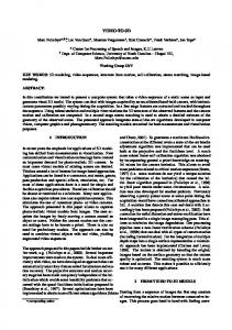
R – reference block, Mi – matched blocks, LN – Local Neighborhood
mean that the block is in the same temporal plane (frame), t3 , and its upper-left element is positioned at spatial
LN
LN M0
M1
LN M3
M2
R
LN
coordinate t1 , t2 . For every processed location t ∈ V , we do the following steps. For each s = s ′, s ′′, s ′′′ ∈ S, we apply the block-matching procedure in order to find s ′′′ blocks of size s ′ × s ′′ which are highly correlated to the reference one, located at t. The search is done within a spatial local neighborhood of size N s × N s among s ′′′ frames centered about the temporal coordinate of the current location (see Figure 1). We form 3D arrays Bt , s∈S by stacking the
R Mi
3D Local Denoising R Mi
matched blocks for each s ∈ S. Then we select an optimal, according to the ICI rule, 3D window size sopt ,t ∈ S. We filter locally the selected 3D array, Bt , sopt ,t , by hard-
LN
thresholding in a 3D transform domain. An inverse transform of the thresholded coefficients reconstructs a local estimate of the noise-free signal in Bt , sopt ,t ,
(( (
)
Bˆt , sopt ,t = F3 D −1 T F3 D Bt , sopt ,t , λthr
)) , (1)
is the characteristic function of the coordinates of the elements in Bˆt , sopt ,t .
relevancy of the reconstructed local estimates, we define a weight, 1 wt = , (2) N har
In the sub-sections to follow, we describe in detail the block-matching and the algorithm for optimal windowsize selection.
where N har is the number of non-zero transform coefficients after hard-thresholding. Observe that the total residual noise energy of Bˆt , sopt ,t is equal to σ n2 N har . Thus,
2.1. Block-matching
Block-matching is employed to find blocks that exhibit high correlation to a given reference block. Because the accuracy of this operation is impaired by the presence of noise, we utilize a block-similarity measure which performs coarse initial denoising in local 2D transform domain prior to matching. Hence, we define a blockdistance measure (inversely proportional to similarity) as
3D arrays with sparser decompositions (i.e. smaller N har ) are awarded greater weights by (2). After processing all locations t ∈ V , the reconstructed local estimates Bˆ , t ∈ V , in general, form an t , sopt ,t
overcomplete representation of the video signal due to an overlap between them. In order to produce the final estimate of the noise-free video data, we aggregate the local estimates from (1) by a weighted average at the positions where they overlap. Thus, we compute xˆ as ∑ w Bˆ ( k ) t∈V
∑ w χ (k ) t∈V
t
,
M3
M2
overlaps k and zero otherwise, and where χ t : V → {0,1}
is the number of elements in Bt , sopt ,t . In order to reflect the
xˆ ( k ) =
LN
(2)
)
t , sopt ,t
R
LN
Figure 1. Example of searching for similar blocks with blockmatching. The 3D array of size selected according to the ICI rule is then denoised in a local 3D transform domain.
threshold from [5], λthr σ n 2 ⋅ log Bt , sopt ,t , where Bt , sopt ,t
t
M0
M1
where F3D is a 3D unitary transform operator and T is a hard-thresholding operator based on the universal
(
LN
(
)
( ( )
) ( ( )
′ − T F2 D Bt2 , λthr ′ d Bt1 , Bt2 = T F2 D Bt1 , λthr
)
, 2
where F2D is a 2D unitary transform operator and Bt1 and Bt2 are arbitrary blocks (2D patches) located at t1 and t2 ,
respectively. Thus, we apply block-matching in order to find the blocks with smallest d -distance to the currentlyprocessed one.
∀k ∈ V ,
t
where Bˆt , sopt ,t ( k ) is an estimate of x ( k ) if its support
-2-
D. Rusanovskyy, K.Dabov, and K. Egiazarian,
VPQM'06, Scottdale, USA, 2006
3. −Dj
j
−I j
4.
Bt ,s2 Bˆt ,s1
The adaptive window size is defined as the largest window size whose confidence interval intersects with the confidence intervals of all smaller window sizes. As a result, the signal within the selected 3D array is characterized by a desired (controlled) level of homogeneity in both spatial and temporal dimensions. Therefore, a unitary transform can effectively decorrelate the true-signal energy in it.
Bˆt ,s2
Bt ,s3
Figure 2. Selection of an optimal 3D window size according to the ICI rule.
3. RESULTS
We evaluate the performance of the proposed denoising algorithm for a few standard grayscale video signals: Salesman, Tennis, and Flower. In Table 1, we present the output ISNR results of: the proposed method, Soft3D [1], WRSTF [2], and 3DDCT [3]. In Figure 3, we compare the PSNR-per-frame results of these methods for Salesman. In our experiments we used the 2D DCT and the 3D DCT for the transform operators F2D and F3 D , respectively. We have chosen DCT because of its good decorrelation ability and the availability of fast algorithms for lengths that are powers of 2. We conducted all experiments with the following fixed settings. The set of predefined 3D window-sizes was S = { 4, 4,8 , 8,8,8 , 16,16,8 }. The ICI rule’s parameter
2.2. ICI rule for optimal window-size selection
In order to adapt to the structures of the underlying signal, we use variable-sized 3D windows for denoising. The variable sizes help to avoid the unwanted presence of details which are not sparsely represented in transform domain (e.g. singularities and edges). Hence, by improving sparsity, we achieve better noise attenuation and improved detail preservation. We use the ICI rule [6] to determine an optimal 3D window-size for each processed location. Recall that for every processed location t ∈ V , by block-matching, we obtain S 3D arrays Bt , s j ∈S whose
was λ = 1.5. For block-matching, we used a spatial local neighborhood with length of the side N s = 15. In order to restrict complexity, we process the locations t ∈ V in both spatial dimensions by sliding to every next processed location with a fixed step p which we denominate as “sliding step”. Hence, it controls the overlap between adjacently processed blocks. We did experiments for full-sliding ( p = 1) type of processing which is characterized by plenty of overlapping local estimates, thus a high level of overcompleteness. In spite of the high computational demand for such kind of processing, we show that the denoising results of this approach (labeled 3D-T1 in Table 1) are superior to the results of all other techniques. We demonstrate the complexity scalability of our method in case of a larger sliding step, p = 4 (see 3D-T4 in Table 1). It results in a 16-times decrease of the complexity as compared to the case of p = 1. We show a fragment of a noisy and denoised 11th frame of Salesman in Figure 3. The sharp details are wellpreserved and also no visible artifacts are present in our estimate.
sizes s j ∈ S are the ordered elements of S. The mean estimator applied on Bt , s j gives
( )
Bt , s j = mean Bt , s j ,
(3)
with variance
σ B2
t ,s j
=
σ n2 s ′j s ′′j s ′′′j
.
The largest index j for which I j is non-empty
determines the selected window size sopt ,t = s j .
Bˆt ,s3
Bt ,s1
Check the intersection of the confidence intervals
I j = ∩ i =1 Di for each s j , where j = 1… S .
(4)
We use the variance to determine a confidence interval D j for Bt , s j . Thus, we define D j as D j = ⎡ Bt , s j − λ ⋅ σ Bt ,s , Bt , s j + λ ⋅ σ Bt ,s ⎤ , (5) ⎢⎣ j j ⎥ ⎦ where λ > 0 is a fixed parameter. We apply the ICI rule for adaptive 3D window size selection as following (see Figure 2 for details). 1. Pre-compute the mean estimator’s variances for each element of S as given by (4). 2. For every processed location t ∈ V , compute Bt , s j and the corresponding confidence intervals D j as
defined in Equations (3) and (5), respectively, for each s j ∈ S.
-3-
D. Rusanovskyy, K.Dabov, and K. Egiazarian,
VPQM'06, Scottdale, USA, 2006
The results demonstrate that the proposed algorithm outperforms all other, known to the authors, video denoising methods, both in terms of PSNR and visual quality. Moreover, the method allows for effective computational scalability as a tradeoff between denoising performance and computational complexity.
36 34
PSNR,dBs
32 30 Noisy 3D−T1 SW 3DDCT WRSTF Soft3D
28 26 24 22
5
10
15 frames
20
25
5. REFERENCES
[1] W.I. Selesnick and K.Y. Li, “Video denoising using 2d and 3d dualtree complex wavelet transforms,” in Wavelet Applications in Signal and Image Processing, Proc. SPIE 5207, San Diego, USA, August 2003.
30
Figure 3. PSNR-per-frame comparative results for Salesman corrupted with additive WGN with σ n = 20.
[2] V. Zlokolica, A. Pizurica and W. Philips, ”Wavelet Domain Noise-Robust Motion Estimation and Noise Estimation for Video Denoising,” First International Workshop on Video Processing and Quality Metrics for Consumer Electronics, Scotssdale, Arizona, USA, January 23-25, 2005. [3] D. Rusanovskyy and K. Egiazarian, ”Video Denoising Algorithm in Sliding 3D DCT Domain,” in Proc. of Advanced Concepts for Intelligent Video Systems, ACIVS 2005, Antwerp, Belgium, September 20-23, 2005. (a)
(b)
[4] JVT of ITU-T and ISO/IEC JTC 1, “Draft ITU-T Recom. and Final Draft Int. Standard of Joint Video Specific. (ITU-T Rec. H.264 | ISO/IEC 14496-10 AVC)”, document JVT-G050r1, May 2003; and Fidelity Range Extensions documents JVT-L047 (non-integrated form) and JVT-L050 (integrated form), July 2004.
(c)
Figure 4. Fragment of the 11th frame of Salesman: (a) original, (b) noisy, σ n = 20, PSNR 22.35 dB, (c) denoised by 3D-T1, PSNR 34.27 dB.
4. CONCLUSIONS
[5] D.L. Donoho, “De-noising by soft-thresholding,” IEEE Trans. on Information Theory, vol. 41, no. 3, pp. 613-627, May 1995.
Considering the sparsity of the transform-domain representations of 3D arrays as a key factor influencing the performance of our transform-based scheme, we do local filtering in moving, varying in size 3D windows. This results in good decorrelation of the noise-free signal in a local 3D unitary transform domain, hence the good detail preservation and effective noise suppression of our technique.
[6] V. Katkovnik, “A new method for varying adaptive bandwidth selection,” IEEE Trans. on Signal Processing, vol. 47, pp. 2567-2571, September 1999.
Table 1. Results in output ISNR (dB).
Video sequence Salesman Tennis Flower
Noise σ n /PSNR 15/24.64 20/23.12 15/26.02 20/22.15 15/25.33 20/23.25
Soft3D [1] 8.57 9.65 5.23 6.43 2.8 2.57
-4-
WRSTF [2] 9.19 10.05 5.49 6.53 3.31 3.95
ISNR (dB) 3DDCT [3] 10.11 10.94 6.17 7.07 4.04 4.62
3D-T1
3D-T4
10.94 11.68 6.47 7.36 4.80 5.14
10.03 10.82 5.95 6.91 4.27 4.48