MR IMAGE COMPRESSION BY HAAR WAVELET ... - DSP

MR IMAGE COMPRESSION BY HAAR WAVELET TRANSFORM E. Hostalkova and A. Prochazka

Institute of Chemical Technology in Prague, Dept of Computing and Control Engineering Technicka 1905, 166 28 Prague 6, Czech Republic Phone: +420 220 444 198, Fax : + 420 220 445 053, Web: dsp.vscht.cz E-mail : [email protected], [email protected]

Abstract: Image compression and coding form substantial problems in many engineering and biomedical applications. This paper is devoted to the study of the multiresolution approach to this problem employing the Haar wavelet transform. In the initial part of the paper, the computation algorithm of the Haar transform (HT) for signals and images is proposed. Then we focus on the orthonormality property of discrete transforms in general. This property fulfilled also by the HT implies preserving the total amount of signal or image energy in its transform coefficients, as formulated by Parseval’s theorem. According to this principle, we may calculate the proportion between the energies conveyed in each coefficients set and the energy of the original image. These percentual proportions indicate the extent of possible image compression. Apart from that, the orthogonality property guarantees reconstruction of a signal or an image from its transform coefficients without any distortion. In the final part of the paper, the two perfect reconstruction (PR) conditions for both the decomposition and reconstruction filters are derived employing the z-transform theory. It is shown, that the Haar filters satisfy the PR conditions. Keywords: Wavelet transform, image decomposition and reconstruction, Haar transform, compression, biomedical image processing

1. INTRODUCTION Digital signal and image processing deals with a wide range of important tasks including noise reduction (further described in Newland (1994) and Vaseghi (2006)), feature extraction for subsequent classification, restoration of missing or corrupted signal or image components. Other challenging problems are introduced with image compression and coding. As proposed by many scientists and mathematicians, a possible solution of the previously mentioned problems consists in multirate or wavelet analysis. From many, let us mention J. Wang and H. K. Huang (1996), G. Menegaz and L. Grewe and J. P. Thiran (2000), Breakspear et al.

(2004), Kingsbury (2001), Li and Shawe-Taylor (2004), M. Weeks and M. A. Bayoumi (2002) and Bullmore et al. (2004). This paper focuses on the use of the discrete wavelet transform (DWT) for biomedical image decomposition, reconstruction and compression (see D. Montgomery and F. Murtagh and A. Amira (2003)). As a wavelet function, we appointed the Haar function for its simplicity and other important properties. The initial part of the paper introduces the computation algorithm of the Haar transform (HT) for one-dimensional and two-dimensional signals.

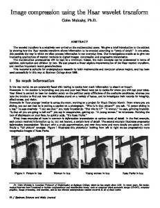
µ (a) SPINAL MR IMAGE

¶ µ ¶ Gn,m Gn,m+1 G1n,m G1n,m+1 = TT(5) Gn+1,m Gn+1,m+1 G1n+1,m G1n+1,m+1

(b) IMAGE CUT

Fig. 1. Real biomedical data representing (a) an axial spine MR image of the size 512 × 512 and (b) its cut of the size 256 × 256 In the following sections, this algorithm is applied to a magnetic resonance (MR) biomedical image presented in Fig. 1. By the means of Parseval’s theorem, we are able to determine the proportion of the energy contained in each individual set of the transform’s coefficients. This information suggests the extent of possible compression.

−1 {x(n)}N n=0 .

Let us have a signal Each pair of its subsequent values {x(n), x(n + 1)} for n = 0, 2, · · · , N − 2 can then be decomposed into two values µ ¶ µ ¶ Xn xn (1) =T Xn+1 xn+1

3. ORTHONORMALITY

A A−1 = A AT = IN

(7)

where IN is an identity matrix of size N × N . In other words, the columns aj for j = 0, 1, 2, ..., N−1 (same as the rows) of A all have unit norms and are perpendicular to each other. These two facts may be expressed by hak , al i =

N −1 X

ak,i al,i = δk,l

(8)

i=0

(2)

Resulting sequence {X0 , X2 , · · · , XN −2 } defines the low-pass decomposition values with its length halved in comparison with the original sequence. The complementary high-pass sequence is composed of values {X1 , X3 , · · · , XN −1 } in the same way. A similar principle can be applied to the analysis of an image [g(n, m)]N,M taking into account that a one-dimensional signal can be interpreted as a special case of an image having one column only. The elementary decomposition element is a 2 x 2 matrix µ ¶ gn,m gn,m+1 (3) gn+1,m gn+1,m+1 where n = 0, 2, · · · , N −2 and m = 0, 2, · · · , M −2. Each such submatrix is decomposed column-wise at first µ ¶ µ ¶ G1n,m G1n,m+1 gn,m gn,m+1 (4) =T G1n+1,m G1n+1,m+1 gn+1,m gn+1,m+1 and then row-wise using relation

This matrix having the half number of rows and columns in comparison with the original one can be used for the next level of decomposition. The results of the 2-D Haar decomposition of the spinal MR image into the first and the second level are presented in Fig. 2.

A real-valued matrix A of size N × N is orthonormal, if its transpose is equal its inverse (see D. B. Percival and A. T. Walden (2000)):

2. HAAR TRANSFORM IN SIGNAL ANALYSIS

using orthogonal decomposition matrix µ ¶ 1 1 1 T= √ 2 1 −1

In this manner, the first level of the decomposition procedure is completed. The resulting matrix elements may be rearranged to define four submatrices. The low/low-pass submatrix is defined hereby   G0,0 G0,2 · · · G0,M −2  G2,0 G2,2 · · · G2,M −2    (6)   ··· GN −2,0 GN −2,2 · · · GN −2,M −2

where the angle brackets denote the inner product and δk,l stands for the Kronecker delta function defined by ½ 1 for k = l δk,l = (9) 0 for k 6= l By multiplying the orthonormal matrix A and a segment of a discrete signal x of size N × 1, we acquire the coefficients vector w of the same size: w=A x

(10)

And reversely, the original sequence x can be synthesised using the relation x = A−1 w = AT w

(11)

4. PARSEVAL’S THEOREM −1 Let us have a discrete signal {x(n)}N n=0 , whose squared norm is given by 2

T

kxk = hx, xi = x x =

N −1 X n=0

x2n

(12)

(a) 1−LEVEL DECOMPOSITION

98.5%

0.7%

(b) 2−LEVELS DECOMPOSITION 94.2%

2%

2%

0.7%

0.4%

(1) Filtering process: As presented by the scheme in Fig. 3, the signal x(n) is passed through a low-pass decomposition filter with an impulse response ld (n) impersonating the scaling function. This can be expressed as a convolution yl (n) =

0.8%

0.1%

0.8%

This equation also represents the total amount of energy εx contained in the signal x(n), hence we obtain: εx = kxk2 (13) Let us consider an arbitrary orthonormal transform employed on x as defined in Eq. (10). The following relation reveals a very important property of all orthonormal transforms, which is preserving the energy εx in its coefficients w: εw = kwk2 = wT w = (A x)T A x = = xT AT A x = xT x = kxk2 = εx

(14)

To summarise these findings, Parseval’s theorem states that the total amount of energy εx contained in the discrete time signal x is equal to the total energy of its orthogonal transform coefficients w: N −1 N −1 X X εx = |xn |2 = wk2 (15) n=0

k=0

Using this relation, we may calculate the energy contained in the original image and also in each of the subimages produced by the Haar transform of each level, as shown in Fig. 2. For more information on Parseval’s theorem, see D. B. Percival and A. T. Walden (2000). The proportions of energy may further be exploited for evaluation of the entropy with a given quantisation step, and thus determining the decrease in the number of bits per pixel in comparison with the original image (see Nick Kingsbury (2006)). 5. PERFECT RECONSTRUCTION In order to derive the perfect reconstruction conditions, we introduce the algorithm for discrete wavelet analysis and synthesis of a sequence −1 {x(n)}N n=0 using an arbitrarily chosen set of filters. Let N be a power of two so as it best suits the purposes of the DWT. Signal decomposition:

ld (k)x(n − k)

(16)

k=0

0.1%

Fig. 2. The Haar transform decomposition of the MR image presenting decomposition (a) up to the first level and (b) up to the second level displaying the percentual proportions of energy conveyed in the subimages

M −1 X

where M is the filter order and the filter output yl (n) is of the same length as x(n). When the ztransform is applied, the convolution becomes a multiplication of the corresponding Z-transform pairs Yl (z) = Ld (z)X(z) (17) Analogously, the signal is passed through a highpass filter hd (n) representing the wavelet function yh (n) =

M −1 X

hd (k)x(n − k)

(18)

k=0

which in z-domain corresponds to Yh (z) = Hd (z)X(z)

(19)

(2) Downsampling by 2 : Then both yl (n) and yh (n) are downsampled by two leaving out every other sample to obtain the detail and the approximation DWT coefficients of the first level, w1a and w1d , respectively, given by w1a = {yl (0), yl (2), yl (4), ..., yl (N −2)} w1d

(20)

= {yh (0), yh (2), yh (4), ..., yh (N −2)} (21)

Steps 1 and 2 may be subsequently repeated many times, until there is only a single sample left. Each such repetition represents another decomposition level. However, for various applications in practise, we most frequently use a maximum of four analysis levels. To keep our description concise, we consider only a single-level decomposition and reconstruction. Signal reconstruction: To reconstruct the signal x(n) from its DWT coefficients, we employ the following techniques: (3) Upsampling by 2 : Upsampling by two means here inserting a zero sample between every two original samples (wavelet coefficients) obtaining ybl (n) = {yl (0), 0, yl (2), 0, ..., yl (N −2), 0} (22) ybh (n) = {yh (0), 0, yh (2), 0, ..., yh (N −2), 0}(23) Apparantly, these two sequences are identical to yl (n) and yh (n) from step 1, respectively, for even indices of n and have zeros for odd values of n. The z-transform of ybl (n) runs as follows

Low−pass filter

Downsampling by 2

yl (n)

Ld (z)

Yl (z)

Original signal

Approximation coefficients

2

w1a

Upsampling by 2

2

Low−pass filter

yˆl (n) Yˆl (z)

Lr (z) Reconstructed signal

x ˆ(n)

x(n) X(z)

High−pass filter

Downsampling by 2

yh (n)

Hd (z)

Yh (z)

2

Detail coefficients

w1d

DECOMPOSITION

Upsampling by 2

yˆh (n)

2

Yˆh (z)

High−pass filter

ˆ X(z)

Hr (z)

RECONSTRUCTION

Fig. 3. A subband coding scheme representing the DWT single-level decomposition and reconstruction of a given signal x(n) Ybl (z) =

∞ X

ybl (n)z −n =

n=0

= yl (0)z 0 +yl (2)z −2 +· · ·+ yl (N −2)z N−2 = 1 = [ [yl (0)+yl (0)]z 0 +[yl (1)−yl (1)]z −1 +· · · 2 · · ·+[yl (N−1)−yl (N−1)]z −(N−1) ] = (24) ∞ ∞ X 1 X = [ yl (n)z −n + yl (n)(−1)−n z −n ] = 2 n=0 n=0 1 = [Yl (z) + Yl (−z)] 2 And similarly for the high-pass sequence 1 Ybh (z) = [Yh (z) + Yh (−z)] 2

(25)

The upsampled sequences ybl (n) and ybh (n) are convolved with the low-pass Lr (n) and the highpass Hr (n) reconstruction filters, respectively. In the z-domain, this procedure produces (26) (27)

(5) Summation: The z-transform of the reconstructed signal is produced by the relation b bl (z) + X bh (z) = X(z) =X 1 = Lr (z)[Yl (z)+Yl (−z)] + 2 1 + Hr (z)[Yh (z)+Yh (−z)] 2

Should the original signal be reconstructed with b no distortion, then X(z) ≡ X(z), which implicates these two perfect reconstruction (PR) conditions: Lr (z)Ld (z) + Hr (z)Hd (z) ≡ 2

(4) Filtering process:

bl (z) = 1 Lr (z)[Yl (z) + Yl (−z)] X 2 bh (z) = 1 Hr (z)[Yh (z) + Yh (−z)] X 2

1 b X(z) = Lr (z)[Ld (z)X(z)+Ld (−z)X(−z)] + 2 1 + Hr (z)[Hd (z)X(z)+Hd (−z)X(−z)] = 2 1 = X(z)[Lr (z)Ld (z)+Hr (z)Hd (z)] + (29) 2 1 + X(−z)[Lr (z)Ld (−z)+Hr (z)Hd (−z)] 2

(28)

Substituing (17) and (19) into the previous equation yields

(30)

Lr (z)Ld (−z) + Hr (z)Hd (−z) ≡ 0 (31) The term X(−z) in (29) is responsible for aliasing due to downsampling by two in step 2. When the condition (31) is fulfilled, this term is cancelled out. Therefore, this condition is sometimes called the anti-aliasing condition. The Haar transform matrix T is given by relation (2). Its√first row represents the low-pass filter ld √ = 1/ 2 [1, 1] with its z-transform pair Ld = 1/ 2 (z −1 + 1). Similarly, the second line √ stands for the high-pass filter h = 1/ 2 [1, −1] d √ with its z-transform Hd = 1/ 2 (z −1 − 1). Since T is orthonormal and also symmetric, its inverse can be expressed as T−1 = TT = T Hence the Haar reconstruction filters lr and hr are identical to ld and hd given by the matrix T, respectively, except the inverse time course. The filters are Lr = √ √ z-transforms of the synthesis 1/ 2 (z + 1) and Hr = 1/ 2 (z − 1). Let us verify that these filters satisfy the PR conditions, first, by substituting into Eq. (30): L r (z)Ld (z) + Hr (z)Hd (z) = 1 1 1 1 = √ (z+1) √ (z−1+1) + √ (z−1) √ (z−1−1) = 2 2 2 2 1 = [1+z+z−1+1+1−z−z −1+1] = 2 (32) 2

(a) 1−LEVEL DECOMPOSITION

(b) RECONSTRUCTION

References

M. Breakspear, M. Brammer, E. Bullmore, P. Das, and L. Williams. Spatiotemporal Wavelet Resampling for Functional Neuroimaging Data. Human Brain Mapping, 23(1):1–25, 2004. E. Bullmore, J. Fadili, V. Maxim, L. Sendur, J. Suckling B. Whitcher, M. Brammer, and M. Breakspear. Wavelets and Functional Magnetic Resonance Imaging of the Human Brain. NeuroImage, 23(Sup 1):234–249, 2004. D. B. Percival and A. T. Walden. Wavelet Methods for Time Series Analysis. Cambridge Series Fig. 4. The Haar transform reconstruction of in Statistical and Probabilistic Mathematics. the MR image presenting (a) decomposition Cambridge University Press, New York, U.S.A, coefficients of the first level and (b) the 2000. reconstructed image D. Montgomery and F. Murtagh and A. Amira. and second, by substituting into the anti-aliasing A Wavelet Based 3D Image Compression Syscondition in Eq. (31): tem. In Proceedings of the Seventh International Symposium on Signal Processing and Its AppliL r (z)Ld (−z) + Hr (z)Hd (−z) = cations, volume 1, pages 65 – 68. IEEE, 2003. 1 1 1 1 G. Menegaz and L. Grewe and J. P. Thiran. Multi−1 −1 = √ (z+1) √ (−z +1) + √ (z −1) √ (−z −1) = rate Coding of 3D Medical Data. In Proceedings 2 2 2 2 of the 2000 International Conference on Image 1 = [−1+z −z−1+1−1−z+z−1+1] = 0 (33) Processing, volume 3, pages 656 – 659. IEEE, 2 2000. To conclude this section, we may state that the J. Wang and H. K. Huang. Medical Image ComHaar filters satisfy both of the PR conditions depression by Using Three-Dimensional Wavelet rived above. To illustrate this fact, we carried out Transform. IEEE Transactions on Medical a single-level decomposition and reconstruction Imaging, 15(4):547 – 554, 1996. of the MR image displayed in Fig. 1b using the N. Kingsbury. Complex Wavelets for Shift InvariHT. The result is displayed in Fig. 4b. The mean ant Analysis and Filtering of Signals. Journal square error calculated for these two images equals of Applied and Computational Harmonic Analzero. For more details on PR conditions, see Nick ysis, 10(3):234–253, May 2001. Kingsbury (2006). S. Li and J. Shawe-Taylor. Comparison and Fusion of Multiresolution Features for Texture Classification. Pattern Recogn. Lett., 25, 2004. 6. CONCLUSION M. Weeks and M. A. Bayoumi. ThreeDimensional Discrete Wavelet Transform ArchiIn this study, we introduced the Haar transform tectures. IEEE Transactions on Signal Process(HT) as a very simple and useful tool for iming, 50(8):2050 – 2063, 2002. age compression and focused on its computation D. E. Newland. An Introduction to Random Vialgorithm. We also discussed the orthonormality brations, Spectral and Wavelet Analysis. Longproperty of discrete transforms along with its reman Scientific & Technical, Essex, U.K., third lationship with Parseval’s theorem, which enables edition, 1994. us to compute the amount of energy contained Nick Kingsbury. 4F8 Image Coding Course. in the decomposition coefficients suggesting the http://cnx.org/, June 2006. extend of image compression. As an orthonormal Saeed Vaseghi. Advanced Digital Signal Processtransform, the HT produces perfect reconstrucing and Noise Reduction. John Wiley & Sons, tion from its coefficients. In the final part of the West Sussex, U.K., third edition, 2006. paper, this crucial property was derived in general using the means of z-transform. Our future studies will be devoted to compression of volumetric biomedical structures and image coding. ACKNOWLEDGMENTS The work has been supported by the research grant of the Faculty of Chemical Engineering of the Institute of Chemical Technology, Prague No. MSM 6046137306.