MRCSI: Compressing and Searching String Collections with Multiple ...

MRCSI: Compressing and Searching String Collections with Multiple References Sebastian Wandelt and Ulf Leser Humboldt-Universitat ¨ zu Berlin, Wissensmanagement in der Bioinformatik, Rudower Chaussee 25, 12489 Berlin, Germany {wandelt, leser}@informatik.hu-berlin.de ABSTRACT

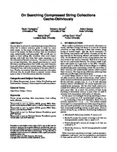
read within the sequenced genome [14]. This problem, called read mapping, amounts to perform a k-approximate search for each read in the genome. In entity search, one needs to find the named entities in text collections despite spelling variations [3]. For instance, the Technische Universit¨at Berlin could be represented as ’Technische-Universit¨at Berlin’, ’Technische-Universitaet Berlin’, or ’Technische- Universit¨at in Berlin’. Such problems also frequently occur in series of Wikipedia versions [24, 26]. Given a set of versions, the task is to find all k-approximate occurrences of the entity in the collection. Standard approximate string search methods create an index on either 1) each string in a collection separately or 2) a concatenation of all strings. Both approaches typically lead to an index that is larger than the sum of the length of all indexed strings. However, in applications like those just described, the indexed documents are highly similar to each other, which can be exploited to drastically reduce index sizes and indexing times. A number of methods have been proposed recently that first referentially compress each string in the collection against a pre-selected reference string [37, 38]. Then, searching is split up into two subtasks: 1) search the reference string and 2) search all deviations of strings from the reference as encoded by referential compression. However, all these methods are only applicable if all indexed strings are highly similar to each other. This is, for instance, a problem when indexing genomes, since compressing a set of human genomes actually means compressing 24 sets of highly similar chromosomes with almost no similarity between the sets. Another problematic scenario for these methods are histories of Wiki sites, as storing them requires methods that can deal with a changing set of pages, as pages may be removed or added. A second problem with being restricted to a single reference is that these methods cannot exploit similarities in-between the compressed strings – but only similarities between those strings and the reference. Consider consecutive versions of Wikipedia articles: Typically, each version is very similar to its version neighbours, but the first recorded version is usually quite different from the most recent one, and no single version (i.e. potential reference) is similar to all other versions. In this paper, we propose the Multi-Reference Compressed Search Index (MRCSI) which is capable of working with multiple references to increase compression rates, chooses these references automatically, and also provides fast approximate search. The fundamental idea is simple (see Figure 1): MRCSI builds a compression hierarchy where strings are compressed w.r.t. various other strings. Implementing this idea yields a number of challenges, in particular to find appropriate algorithms and data structures (a) for allowing high compression speed, (b) for choosing the best compression hierarchy in terms of space, and (c) for achieving efficient k-approximate search in a given compression hierarchy. Our paper

Efficiently storing and searching collections of similar strings, such as large populations of genomes or long change histories of documents from Wikis, is a timely and challenging problem. Several recent proposals could drastically reduce space requirements by exploiting the similarity between strings in so-called referencebased compression. However, these indexes are usually not searchable any more, i.e., in these methods search efficiency is sacrificed for storage efficiency. We propose Multi-Reference Compressed Search Indexes (MRCSI) as a framework for efficiently compressing dissimilar string collections. In contrast to previous works which can use only a single reference for compression, MRCSI (a) uses multiple references for achieving increased compression rates, where the reference set need not be specified by the user but is determined automatically, and (b) supports efficient approximate string searching with edit distance constraints. We prove that finding the smallest MRCSI is NP-hard. We then propose three heuristics for computing MRCSIs achieving increasing compression ratios. Compared to state-of-the-art competitors, our methods target an interesting and novel sweet-spot between high compression ratio versus search efficiency.

Keywords Indexing, compression, dissimilar strings

1.

INTRODUCTION

Information systems for strings are an old [19], yet still highly relevant research topic. The two most fundamental problems for such systems are storage efficiency and search efficiency: How can large string collections be stored in as little space as possible while still performing string searching as fast as possible. One particularly important type of search is k-approximate substring search: Given the collection of strings S and a query q, find all substrings of strings in S similar to q within a given error threshold k. Several applications exist for which scalability of such operations is tremendously important. We give two examples. In Bioinformatics, next generation sequencing produces billions of DNA sequences (called reads) in a single day, each between 50 and 400 characters long. Analyzing this data first requires to determine the position of each This work is licensed under the Creative Commons AttributionNonCommercial-NoDerivs 3.0 Unported License. To view a copy of this license, visit http://creativecommons.org/licenses/by-nc-nd/3.0/. Obtain permission prior to any use beyond those covered by the license. Contact copyright holder by emailing [email protected]. Articles from this volume were invited to present their results at the 41st International Conference on Very Large Data Bases, August 31st - September 4th 2015, Kohala Coast, Hawaii. Proceedings of the VLDB Endowment, Vol. 8, No. 5 Copyright 2015 VLDB Endowment 2150-8097/15/01.

461

a) Collection of heterogeneous strings Kohala Coast-Hawaii Koala Coast Koala Coast/Hawaii Kola CoasthHawaii Orchid Island Orchied Island

b) Compression against a single reference

c) Compression hierarchies

Kohala Coast-Hawaii 2

Koala Coast 3

Kohala Coast-Hawaii Orchid Island

Koala Coast/Hawaii 3

Orchied Island

Kola CoasthHawaii

9 10

Koala Coast

2 2

Orchid Island Orchied Island

2

Koala Coast/Hawaii 3

Kola CoasthHawaii

Figure 1: Basic idea of multi-reference referential compression. Boxes are to-be-compressed strings, edges represent referential compression; for instance, s=’Koala Coast’ could be represented with reference t=’Kohala Coast-Hawaii’ as [(0, 2), a, (4, 8)], indicating that s = t(0, 2)◦ a ◦t(4, 8). Numbers in circles show the number of entries in the compressed representation. Description: a) Collection of dissimilar strings. b) Prior work uses only one reference. Compression potential is lost. (c) Compression hierarchies exploit identical substrings.

provides solutions to all these challenges: 1. We develop a framework for multiple reference compressed search indexes (MRCSIs) for any kind of strings, e.g. text, biological sequences, and semi-structured documents. 2. The question arises which MRCSI is the best. We present a theoretical model for estimating the size of a given MRCSI. 3. We prove that finding the space-optimal MRCSI is NP-hard. 4. We propose three heuristics of increasing complexity for creating a MRCSI from a given string collection: Starting from flat compression forests over general compression forests to DAG-structured compression hierarchies. In all these settings, reference strings are picked automatically. 5. Experimental results on real-world datasets show that our heuristics build indexes up to 90% smaller than the state-ofthe-art while providing comparable search times. The rest of this paper is structured as follows: We review related work in Section 2. A formalization of string databases and referential compression is defined in Section 3. We present our framework for multi-reference compressed search indexing in Section 4 and also prove that finding the most compact MRCSI under a certain, intuitive cost model is NP-hard. We introduce three heuristics for building increasingly complex MRCSIs in Section 5. We report on experimental results and compare our algorithms to the most related approaches in Section 6. The paper concludes in Section 7.

2.

does not directly support approximate search; in Section 6, we will compare against a modified version of this tool which does allow searching. A technique for increasing the compression ratio of RLZ-based compression was proposed recently [34]: By eliminating rarely used parts from the dictionary, significant improvements over the compression ratios are reported, but - as RLZ - without a search index. Compressed Indexing in Specific Domains: Managing string collections is particularly important in Bioinformatics. Several algorithms recently emerged that compress a set of genomes against a reference. GenomeCompress [38] creates a tree representation of differences between a collection of genomes using an alignment technique. In our prior work, we presented RCSI [37] which uses an alignment-free referential compression algorithm [36] and additionally builds a compressed index for allowing approximate searches. We showed that RCSI outperforms GenomeCompress by at least an order of magnitude. Three very recent proposals are [6, 10, 33], which either 1) achieve impressive compression rates but exploit the existence of a multiple sequence alignment for all strings [6, 10] (very time consuming for long/many strings), or 2) do not find all matches for a given query [33], since they only construct a so-called pan-genome, which contains less information than the collection of sequences [6]. Theoretical Computer Science: Given upper bounds on pattern lengths and edit distances, [11] preprocesses the to-be-indexed text with LZ77 to obtain a filtered text, for which it stores a conventional index. But [11] has not been demonstrated to scale up to multi-gigabyte genomic data [6]. Grammar-based compressors, as XRAY [2], RE-PAIR [22], and the LZ77-based compressor LZEnd [20], have enormous construction requirements, limiting their application to small collections. Other work addresses related problems over highly-similar sequence collections, e.g., document listing [12] and top-k-retrieval [27].

RELATED WORK

We give an overview on prior work concerning string compression algorithms and report how compression techniques are used for solving indexing/approximate search problems over document collections in different areas. String Compression: Compression has a long tradition in computer science and related areas. A relative novel development are referential compression algorithms [7, 17, 21, 30, 36] which encode (long) substrings of the to-be-compressed input with reference entries to another fixed string, called the reference. The compression ratio of these methods grows with increasing similarity between to-be-compressed strings and the reference and can skyrocket for very similar strings [8, 35]. For instance, standard compression schemes achieve compression rates of 4:1–8:1 for DNA sequences, while referential compression algorithms reach compressions rates of more than 1,000:1 [7, 36] when applied to a set of human genomes. Compressing Semi-Structured Documents: Compressed inverted text indexes [4, 29] are used for indexing versioned documents. The general idea is to compress the list of occurrences for each word using a standard compression algorithm, for instance, PFORDELTA [39]. RLZ [16, 17] is a tool for referentially compressed storage of web-collections achieving high compression ratios, but

3.

PRELIMINARIES

A string s is a finite sequence of characters from an alphabet Σ. The concatenation of two strings s and t is denoted with s ◦ t. A string s is a substring of string t, if there exist two strings u and v (possibly of length 0), such that t = u ◦ s ◦ v. The length of a string s is denoted with |s| and the substring starting at position i with length n is denoted with s(i, n). s(i) is an abbreviation for s(i, 1). All positions in a string are zero-based, i.e., the first character is accessed by s(0). Given strings s and t, s is k-approximate similar to t, denoted s ∼k t, if s can be transformed into t by at most k edit operations (replacing one symbol in s, deleting one symbol from s, adding one symbol to s). Given a string s and a string q, the set of all k-approximate matches in s with respect to q, denoted search(s)kq ,

462

Algorithm 1 Compression against multiple references

1: 2: 3: 4: 5: 6: 7: 8: 9: 10: 11:

One example for a referential compression of s2 against s1 is rcs2 = [(1, 0, 2, a)(1, 4, 7,t)], since we have s2 = s1 (0, 2) ◦ a ◦ s1 (4, 7) ◦ t. Similarly, we can referentially compress s5 against s1 : rcs5 =[(1, 0, 0, O), (1, 0, 0, r), (1, 0, 0, c), (1, 2, 1, i), (1, 0, 0, d), (1, 6, 1, I)(1, 10, 1, l)(1, 3, 1, n)(1, 0, 0, d)]. However, this referential compression is obviously not a good compression, since the number of RMEs (9) is very close to the number of symbols (13) in the original string s5 . Intuitively, we would like to compress strings against similar references only, in order to exploit similarities for compression. Furthermore, exploitation of similarities against multiple references often decreases the number of RMEs further. Below is an example, where s1 and s5 are (uncompressed) references, s2 is referentially compressed against {s1 }, s3 is compressed against {s1 , s2 }, s4 is compressed against {s1 , s2 }, and s6 is compressed against {s5 }: comp(s1 , {s1 }) = [(1, 0, 18, i)] comp(s2 , {s1 }) = [(1, 0, 2, a)(1, 4, 7,t)]

Input: to-be-compressed sequence s and collection of reference sequences REF = {re f1 , ..., re fn } Output: referential compression rcs of s with respect to REF Let rcs be an empty list while |s| 6= 0 do Let pre be the longest prefix of s, such that (pos, pre) ∈ search(re fi )0pre , for a number pos, and there exists no 1 ≤ j ≤ n, with j 6= i and re f j contains a longer prefix of s than re fi if s 6= pre then Add (re fi , pos, |pre|, s(|pre|)) to the end of rcs Remove the first |pre| + 1 symbols from s else Add (re fi , pos, |pre| − 1, s(|pre| − 1)) to the end of rcs Remove the prefix pre from s end if end while

is defined as the set search(s)kq = {(i, s(i, j)) | s(i, j) ∼k q}. This definition is naturally extended to searching a database (or collection) of strings: A string database S is a collection of strings {s1 , ..., sn }. Given a query q and a parameter k, we define the set of all k-approximate matches for q in S as DBsearch(S)kq = {(l, search(sl )kq ) | sl ∈ S}. For example Orchid ∼1 Orchied, because the symbol e can be removed from Orchied with one delete operation to obtain Orchid. If S = {s1 , s2 }, with s1 = Orchid and s2 = Orchied, DBsearch(S)1hid = {(1, {(3, hi), (3, hid), (4, id)}), (2, {(3, hi), (3, hie), (3, hied)})}. Intuitively, the problem we study in this paper is the following: How can we encode a string database S, such that (a) the encoding requires as little space as possible and (b) k-approximate searches can be performed efficiently. The basic technique we use for storing strings in a compact manner is to compress them by only storing differences to other strings, called references [7, 21, 36]. D EFINITION 1 (R EFERENTIAL C OMPRESSION ). Let REF be a set of reference strings and s be a to-be-compressed string. A tuple rme = (re f id, start, length, mismatch) is a referential match entry (RME) if re f id ∈ REF is a (identifier for a) reference string, start is a number indicating the start of a match within re f id, length denotes the match length, and mismatch denotes a symbol. A referential compression of s w.r.t. REF is a list of RMEs rcs = [(re f id1 , start1 , length1 , mismatch1 ), ..., (re f idn , startn , lengthn , mismatchn )] such that (re f id1 (start1 , length1 ) ◦ mismatch1 ) ◦ ...◦ (re f idn (startn , lengthn ) ◦ mismatchn ) = s. The size of a RME (re f id, start, length, mismatch) is defined as length + 1. The offset of a RME rmei in a referential compression rcs = [rme1 , ..., rmen ], denoted o f f set(rcs, rmei ), is defined as ∑ j The resulting M is: {(s1,{(8,oa},(8,oas)})} s1

Kohala Coast-Hawaii

s5

2. Find 1-approximate matches of ‘oad’ in compressed suffix tree of overlaps

Orchid Island

RME propagation map with interval trees for each reference

Components of the search index

Interval tree for s2

(0,18)

s2:3

(4,7)

Interval tree for s5

(0,11)

(13,5)

(0,12) (5,7)

s5:0

(4,7) (0,5)

(0,2) s2:0

(0,2) s3:12 s4:11

s4:0

s4:3

s3:0

s6:0

s6:7

Overlap map for all compressed strings

waii

s1:15

s3:14

Koala

s2:0

land

s5:9

s6:10

oast

s2:7

Kola C

s4:0

asthHaw

chied

s6:2

ast/Haw

s4:7 s3:8

Example for searching ‘oad’ with k=1

Interval tree for s1 s1:0

Query ‘oad’ is split into seeds ‘oa’ and ‘d’, the seeds’ positions retrieved and extended for full 1-approximate matches. This yields the following 1approximate matchs: - (0,oa) and (0,oad) in ‘oast’ Since ‘oast’ is contained in s2 at position 7, we add matches (7,oa) in s2 and (7,oa) in s2 to M - (1,oa) and (1,oal) in ‘Koala’ Since ‘Koala’ is contained in s2 at position 0, we add matches (1,oa) in s2 and (1,oal) in s2 to M

3. Fixed point computation of M with RME propagation maps We have M={(s1,{(8,oa},(8,oas)}),(s2,{(1,oa},(1,oal)})} and set M*=M. The intervals (8,2) and (8,3) are looked up in the interval tree for s1: Both are covered by (0,18) from s1:0 and (4,7) from s2:3. We already have the matches in s1, and thus add only {(s2,{(7,oa},(7,oas)})} to M*. The intervals (1,2) and (1,3) are looked up in the interval tree for s2: Both are covered by (0,11) from s3:0. We add {(s3,{(1,oa},(1,oal)})} to M*. The first iteration is finished and we set M=M*. We only need to check for new {(s2,{(7,oa},(7,oas)})} and {(s3,{(1,oa},(1,oal)})}. Since we have no RME propagation map for s3, the matches for s3 cannot be propagated further. The intervals (7,oa) and (7,oas) are looked up in the interval tree for s2: We have covering intervals (0,11) and (4,7), which lead to the following new matches in M*: {(s3,{(7,oa},(7,oas)})} and {(s4,{(6,oa},(6,oas)})} The second iteration is finished and we set M=M*.

Compressed suffix tree for all concatenated overlaps

Since we have no RME propagation maps for s3 or s4, we are finished. The overall result is: M={(s1,{(8,oa},(8,oas)}),(s2,{(1,oa},(1,oal),(7,oa},(7,oas)}),(s3,{(1,oa},(1,oal), (7,oa},(7,oas)}),(s4,{(6,oa},(6,oas)})}.

waii|land|oast|chied|Koala |Kola C|asthHaw|ast/Haw 0:waii 4:land 8:oast 12:chied 17:Koala 22:Kola C 28:asthHaw 35:ast/Haw

Figure 3: Index example for the compressed strings from Example 1. The left part of the figure visualizes the index components and the right parts sketches the 1-approximate search for query ’oad’. We have created the index with maxql = 3 and maxed = 1. In interval trees, dashed lines denote occurrence annotations.

4.2.3

an efficient technique to find matches in overlaps. Naive traversal over the overlap map at query time is slow, since each overlap string has to be accessed, while often only few overlap strings do contain a match for a seed. Therefore, we create an index for all overlap strings as follows: Given that the overlap map contains strings o1 , ..., on as keys, we create a compressed suffix tree over the concatenation ototal = o1 ◦ ... ◦ on . The overlap map together with the compressed suffix tree for ototal is called indexed overlap map. For very short RMEs and large δ , overlaps can overlap each other, since they are extracted from nearby locations in the strings. Indexing a concatenation of these overlaps possibly leads to a waste of space. It is interesting to address this problem in the future by using an index structure tailored towards storing short and possibly similar strings. However, naive approaches like Patricia tries will not work, since these only identical prefixes are exploited for space reduction. Alternatives are the use of directed acyclic word graphs [13] or partition-based approaches [18]. We leave this analysis for future work. Clearly, using the compressed suffix tree over ototal , we can find all occurrences of seeds in each oi , given a simple data structure which keeps track of the position of each oi in ototal . At search time, we first look up query seeds in the CST of ototal , apply the extend algorithm to find all k-approximate matches (still working on ototal only), then project all matching positions from ototal to the oi , and finally exploit the overlap map to project the matches from oi back to the compressed strings, using location augmentations.

Finding all Matches

The above technique for finding k-approximate matches is still incomplete, since matches have to be propagated along paths in the reference dependency graph. The sound and complete algorithm, therefore, is described next: First, all matches contained in primary references are identified, with seed-and-extend and the compressed suffix trees for primary references. Second, all overlap matches are identified, with seed-and-extend and the compressed suffix tree for all concatenated overlaps. At this stage, we have a set of initial matches in some strings, which we denote with M. These initial matches in M are propagated from references to referential compressions, by exploiting the interval tree: for each match in M, we access the interval tree of the string containing the match and identify all intervals from compressed strings subsuming this match. From these intervals, we reproduce the original occurrence positions of matches and add them to M. After one iteration, we obtain a new M, which contains the initial matches together with the newly derived matches. The procedure is repeated for the new M, until a fixed point is reached, i.e. M does not give rise to new matches regarding the interval trees. E XAMPLE 2 (MRCSI). In Figure 3, we show an example for searching the strings from Example 1 for the query ’oad’ with k = 1. We would like to point out that multiple matches in the reference have to be evaluated and propagated separately, since a non-identical interval in the reference could have different subsuming intervals. Thus, even if the same match is found several times in the reference, they have to be propagated one-by-one.

465

4.2.4

MRCSI

The set of indexed primary references together with an indexed RME propagation map and indexed overlap map yields a multireference compressed search index (MRCSI). D EFINITION 6 (MRCSI). Given string database S = {s1 , ..., sn } and a multi-reference compressed string database mrcsd for S, a multi-reference compressed search index (MRCSI) for S is a tuple mrcsi = (IPREF, rmemap, ovlmap) where IPREF is a collection of compressed suffix trees for the primary references in mrcsd, rmemap is an indexed RME propagation map for mrcsd and ovlmap is an indexed overlap map for mrcsd. A MRCSI index structure contains all necessary for k-approximate search in string collections. We prove soundness and completeness of our search algorithm over MRCSIs. P ROPOSITION 1. Given a string database S = {s1 , ..., sn }, every MRCSI of S finds all k-approximate matches (and only these). P ROOF. k-approximate matches in a compressed string rcs have to either 1) be completely covered by a RME or 2) overlap at least two RMEs. For 1), if the match is contained inside a RME, then it must occur in one of the references of rcs. If the reference is primary, then them match is found via the compressed suffix trees in IPREF and forwarded to rcs with the RME propagation map. Otherwise, the reference is not primary (which is discussed below). For 2), the indexed overlap map contains all overlaps of length up to δ over two or more RMEs. Since a k-approximate match can never be longer than δ , the match is inside the overlap map and propagated to the position of the compressed sequence by using the offset information stored in the interval tree. The remaining case, that the match is completely covered by a RME and reference is not primary, can be shown by induction, since all matches in the non-primary reference are eventually found (induction hypothesis) and the RME propagation map propagates all matches covered by RMEs in rcs to their positions (induction step). The space requirement of the basic MRCSI index structure is determined by the number N of strings, the maximum length L of strings, and their degree of similarity. In the worst-case, all strings are maximum dissimilar, e.g., their alphabets are disjoint, yet all strings are (inefficiently) compressed against the reference. The space complexity is estimated as follows: There exists exactly one reference string re f , with length at most L, and all other N − 1 strings are compressed against re f . In the worst case, each character requires its own RME, yielding at most (N − 1) ∗ L RMEs. The size of the compressed suffix tree for re f is in O(L) and the size of the RME propagation map is in O(L ∗ N), since we have at most L ∗ (N − 1) + 1 RMEs. The size of the overlap map is in O(L ∗ N) as well, since we create one overlap for each RME, all of which are unique. We have O(L ∗ N) augmentations of occurrences in the RME propagation map and in the overlap map. In total, we obtain a worst-case space complexity of O(N ∗ L). The worst-case space complexity is the same as if we create a compressed suffix tree over the concatenation of all strings. We discuss the hardness of creating a space-optimal MRCSI next.

4.3

random strings showed that the size of a compressed psuffix tree for a Σ-string s can be estimated with 8 ∗ |s| ∗ (1.48 + 0.01 ∗ |Σ|) bits. Thus, the size of IPREF plus their suffix ptrees is estimated with COST 1 = ∑s∈IPREF 8 ∗ |s| ∗ (1 + 1.48 + 0.01 ∗ |Σ|). Note that we store the original PREF in addition to the suffix trees, as extracting substrings from a compressed suffix tree is rather slow [36]. Thus, we perform the verification-phase of the seedend-extend algorithm for approximate search on the original string and not on the compressed suffix tree. Indexed RME propagation map: The RME propagation map assigns interval trees with occurrence augmentations to reference sequences. A single interval entry consists of start and length of the interval, which yields 2 ∗ B bits. An occurrence augmentation consists of a string identifier and a position, which sums up to dlog2 (|S|)e + B. The total amount of storage required for a single interval tree is estimated with 2 ∗ N ∗ (2 ∗ B) + Y ∗ dlog2 (|S|)e + B), where N is the number of interval entries in the interval tree and Y is the number of occurrence records in the interval tree. Thus, in total we have COST 2 = ∑z∈Z (2 ∗ Nz ∗ (2 ∗ B) + Yz ∗ dlog2 (|S|)e + B)) bits for storing the RME propagation map, where Z is the set of interval trees, i.e. references in the original MRCSD. Indexed overlap map: The overlap map asserts to each unique overlap string a list of occurrences in compressed strings. A single map entry needs 8 ∗ (δ ∗ 2 + 1) bits for the overlap string and N ∗ (dlog2 (|S|)e + B) bits for the occurrences. In total, the size of the overlap map is estimated with COST 3 = X ∗ (8 ∗ (δ ∗ 2 + 1) +Y ∗ (dlog2 (|S|)e + B)) + ovlcst, where X is the number of unique overlap strings, Y is the number of occurrence records in the domain of the overlap map, i.e., number of RMEs in the original MRCSD, and ovlcst is the estimated length of the CST over all concatenated overlaps. In total, we have an estimated cost (in bits) for a compressed search index of COST ((IPREF, rmemap, ovlmap)) = COST 1 + COST 2 + COST 3. Based on this model, we define the problem of finding the smallest MRCSI for a string database S. D EFINITION 7 (M INIMAL MRCSI). A multi-reference compressed search index mrcsi is minimal for a string database S, if there exists no other mrcsi2 for S with COST (mrcsi2 ) < COST (mrcsi). The MRCSI size optimization problem is to find a minimal mrcsi for a string database S. The MRCSI size decision problem is to decide whether there exists a MRCSI with cost C for S. P ROPOSITION 2. MRCSI size decision problem is NP-hard. P ROOF. First, we show that the problem is in NP. Given a multireference compressed search index mrcsi, we obviously can compute the cost of mrcsi and compare it to C. Now we prove that the problem is NP-complete, by reduction to the Subset-Sum decision problem, which is known to be NP-complete. Given a set of integers I = {i1 , ..., in } and value z, the question of Subset-Sum is whether there exists a subset of I ∗ ⊆ I, with ∑i∈I ∗ i = z. It is easy to see that the decision problem for a simplified COST1-function alone is sufficient to model Subset-Sum. Let COST 2 = COST 3 = 0 and S = {s1 , ..., sn }, such that each string s j has length i j . Furthermore, let COST 1 = ∑s∈PREF |s|. The solution to the MRCSI size decision problem coincides with the Subset-Sum decision problem. Altogether, the MRCSI size optimization problem is NP-hard.

Optimal MRCSI’s

We develop a cost-model for estimating the size (in bits) of a given mrcsi = (IPREF, rmemap, ovlmap) for a string database S. We estimate the overall size by an estimation of the size of each of the three components. In the following we assume that L is the length of the longest string in S. Thus, position values and length values for strings can be stored with B = dlog2 (L)e bits. Primary references: For each (uncompressed) primary reference, we store a compressed suffix tree. Symbolic regression of index sizes for

5.

HEURISTICS FOR COMPUTING MRCSI

Given Proposition 2, it is not possible to design a polynomial-time algorithm for solving the MRCSI size optimization problem, unless P=NP. In this section we develop three heuristics that each considers only a certain subset of all possible MRCSD structures, where the number of possible references is increased from heuristic to heuristic. This also leads to gradually increasing compression ratio

466

Algorithm 2 Computation of MRCSI-CPart

in practice (see Section 6): • Partition (CPart) in Section 5.1: We restrict MRCSI such that each string is compressed against a single primary reference, while there can be several primary references in total. • Compression Forests (CForest) in Section 5.2: We extend CPart to exploit similarities between non-primary references, by introducing a new indexing technique, called compression forests. • Compression DAG (CDAG) in Section 5.3: Compression forests are generalized to directed acyclic graphs. Below, we only describe how to compute PREF and COMP for each heuristic. Computation of (indexed) RME propagation map and (indexed) overlap map is straight-forward and the same for all three heuristics.

5.1

1: 2: 3: 4: 5: 6: 7: 8: 9: 10: 11: 12: 13: 14: 15: 16: 17: 18: 19: 20:

Partition (CPart)

We introduce CPart, a compression strategy that splits a given string database S = {s1 , ..., sn } into a set of primary references and referentially compressed strings, such that each referentially compressed string is encoded w.r.t. exactly one primary reference. Note that finding a minimal such MRCSI is again NP-hard, since SubsetSum can be reduced to this problem (proof omitted for brevity). CPart indexes all strings in the collection S={s1 , ...sn } iteratively. Starting with an empty MRCSD (PREF = 0/ and COMP = 0), / it begins with processing s1 . Since there is no primary reference yet, s1 cannot be compressed against an existing primary reference. We add s1 to PREF, and obtain PREF = {s1 } and COMP = {s1 }4 . Next, we process s2 . We have two options: 1) s2 is added as a new primary reference or 2) s2 is referentially compressed against s1 . Note that we can, in principle, compute the exact storage cost for both options (see Section 4.3) but this would be slow; how this can be approximated efficiently is described below. We choose the option which minimizes storage: If s1 and s2 are rather unrelated, we choose the first option because the referential compression (plus overlaps) would use more space than if we add s2 as a new primary reference. In this case we get PREF = {s1 , s2 } and COMP = {s1 , s2 }; if s1 and s2 are rather similar, we would get PREF = {s1 } and COMP = {s1 , s2 }. When we next add s3 , we have three options: 1) s3 is added as a new primary reference, or 2) s3 is referentially compressed against s1 , or 3) s3 is referentially compressed against s2 . CPart first chooses the primary reference which would allow for the best compression of s3 , i.e., it first chooses among options 2 and 3 and then compares the winner to option 1. The remaining strings are added in the same way. The complete CPart-algorithm is shown in Algorithm 2. To decide which option is the least space-intensive, Algorithm 2 needs to compute the number of RME’s necessary for compressing one string w.r.t. another. We call this property compressibility. This quantity can be computed quickly if the two strings are similar using a technique called local matching optimization [36]. In experiments, we achieved main-memory compression speed of more than 500 MB/s. However, if the to-be-compressed string and the reference have only few similarities, the compression speed degrades recognizably (down to 10-50 KB/s in tests). Algorithm 2 very often has to compute compressibility between probably dissimilar strings. To cope with this issue, CPart only estimates compressibility using N parts of the to-be-compressed string s: s is split into N blocks and the longest prefix of each block is looked up in the existing references. The lengths of the matches are averaged and exploited as an estimation of the average length of the RMEs for the whole strings. In our experiments, we fixed N to log2 (|s|).

Input: String database S = {s1 , ..., sn } Output: MRCSI (IPREF, rmemap, ovlmap) Let PREF = COMP = rmemap = ovlmap = 0/ for 1 ≤ i ≤ n do Let cost1 = ∞ if |PREF| > 0 then Find pre f ∈ PREF such that |comp(si )| is approximately minimal (si is compressed with respect to pref) Let rcs = comp(si ) (si compressed against pre f ) Let cost1 be the cost if rcs is added to MRCSI end if Let cost2 be the cost if si is added as a new primary reference if cost2 > cost1 then Let COMP = COMP ∪ {rcs} else Let PREF = PREF ∪ {si } Let COMP = COMP ∪ {[(si , 0, |si | − 1, si [|si | − 1]])} end if end for Compute IPREF from PREF Compute rmemap from (PREF,COMP) Compute ovlmap from (PREF,COMP) Return (IPREF, rmemap, ovlmap)

This was sufficient to find any reference with sufficient degree of similarity. Obviously, CPart essentially performs a compressibility-based clustering of the strings in the collection. Therefore, existing string clustering techniques might be applicable as well. However, the major challenge in clustering is to define a similarity criterion suitable for the particular problem at hand. A popular choice when clustering strings is the edit distance, but computing it is slow (O(|s1 |∗ |s2 |)), and it is not always positively correlated to compressibility. For instance, the strings s1 = an bn and s2 = bn an have a large edit distance (2 ∗ n), but still a high compressibility, i.e. s2 can be encoded with two RMEs into s1 . Still, it remains an interesting topic for future work to experiment with other, more efficient similarity measures, such as the Jaccard coefficient over q-grams.

5.2

CForest

CPart overcomes the shortcoming of methods like RCSI to use only a single reference during compression. However, each string still is only compressed against a single primary reference. Similarities between compressed strings are not exploited, which neglects ample compression potential. E XAMPLE 3. We have a set of strings S = {s1 , ..., s3} with s1 =Kohala Coast-Hawaii, s2 = Kola CoasthHawaii, s3 =Kola CoasthHawii. We obtain the following referential compression: comp(s2 , {s1 }) =[(1, 0, 2, l), (1, 5, 7, h), (1, 13, 5, i)] comp(s3 , {s1 }) =[(1, 0, 2, l), (1, 5, 7, h), (1, 13, 3, i)(1, 0, 0, i)] If s2 is used as additional reference for s3 , then we obtain the shorter compression for s3 : [(2, 11, 2, l), (1, 13, 3, i)(1, 0, 0, i)], by replacing the identical RME sublist [(1, 0, 2, l), (1, 5, 7, h)] with a reference into s2 . We capture such ideas in so-called second-order compression. In contrast to CPart, second-order compression also considers references into referential compressions instead of only uncompressed strings. This is achieved by greedily rewriting an existing referential compression (against a primary reference) into one against other referential compressions, by replacing consecutive RMEs occurring in the to-be-rewritten compressed string and the compressed reference strings by one second-order RME into the compressed reference string. Indexing RMEs: Given a collection of referential compressions R = {rcs1 , ..., rcsn }, as obtained by CPart, we create a hashmap

4 String s is a primary reference, yet denoted with one RME as a 1 compressed string.

467

Algorithm 3 Rewriting a referential compression against another referential compression

1: 2: 3: 4: 5: 6: 7: 8: 9: 10: 11: 12:

selects the most similar referential compression seen before based on sampling: it selects log2 (n) equally distributed RMEs from a referential compression with n RMEs. For each sample RME, the set of compressed strings containing the RME is computed. The compressed string rcs which contains the highest number of sampled RMEs is identified. The compressed string rcs plus all its parents in the reference dependency graph are set as second-order references for rewriting, following the procedure described above. After compression, the second-order compressed string is added as a child of rcs, thus, preserving a forest structure. The Algorithm is summarized in Algorithm 4. Note that we do not compress the sequences twice against primary references. Although CForest builds on the selection of primary references of CPart (based on compressibility estimation only), the actual compression takes place in Algorithm 4. Overall, CForest tries to rewrite each compressed string only against compressed strings on the same path to the primary reference. Thus, CForest is a compromise: On the down side, it does not consider all possible compressions of sequences of RMEs in the entire MRCSD; but by doing so, it only has to consider few references for rewriting.

Input: To-be-rewritten referential compression rcs j , reference referential compression rcsre f Output: Referential compression result Let result be an empty list of referential match entries while |s| 6= 0 do Let pre be the longest prefix of rcs j , that is an infix of rcsre f if |pre| ≤ 1 then result = result ◦ rcs j (0) Remove rcs j (0) from rcs j else Add (i, o f f set(rcsre f , pre(0)), (∑rme∈pre |rme|) − 1, c) to the end of result, where c is the mismatch character of the last RME in pre Remove the prefix pre from rcs j end if end while Return result

Algorithm 4 Computation of MRCSI-CForest

1: 2: 3: 4: 5: 6: 7: 8: 9: 10: 11: 12: 13:

Input: String database S = {s1 , ..., sn } Output: MRCSI (IPREF, rmemap, ovlmap) Let IPREF be the set of primary references of CPart and COMP the referential compression Let NEWCOMP = 0/ Let rdg be an empty reference dependency graph for 0 ≤ i ≤ |COMP − 1| do Select (by sampling) the most similar referential compression to COMP[i] from COMP[0, i − 1], let the result be rcs Let re f cands be the set containing rcs and all its direct/indirect parents in rdg Rewrite COMP[i] against re f cands and let the result be ncomp Append ncomp to NEWCOMP Add ncomp as a child of rcs in rdg end for Compute newrmemap from (PREF, NEWCOMP) Compute newovlmap from (PREF, NEWCOMP) Return (IPREF, newrmemap, newovlmap)

5.3

CDAG

We implemented a third heuristic, termed Compression DAG (or CDAG). It keeps the general approach of CForest, but now each referential compression is compressed against all previously compressed strings with the same primary reference (induced by CPart) instead of only the best one and its parents. We only perform a single pass over the strings in each partition, which keeps the dependency graph acyclic; the resulting structure is a DAG. The algorithm is very similar to Algorithm 4. The only differences are: re f cands = NEWCOMP replaces Lines 5–6 in Algorithm 4 and the reference dependency graph has to be updated accordingly (Line 9), by adding COMP[i] as a child to all re f cands. Note that CDAG still is heuristic, since is explores only a tiny fraction of the entire search space of all MRCSIs for a given string database; in particular, it is greedy in selecting primary references, and inherits the fairly simple method from CPart which determines the actual number of primary references.

from RMEs to offsets of RMEs in the referential compressions. For each RME in R we store the identifier of the referential compression and offsets where the RME occurs. Second-order compression is implemented, on top of this RME hashmap, with an algorithm very similar to the referential compression algorithm for computing RMEs: We simply replace the alphabet Σ with the set of all RMEs. This idea is implemented in Algorithm 3 for a single compressed reference string. The to-be-rewritten referential compression rcs j is traversed from left to right. The longest prefix of rcs j (i.e., a sequence of RMEs) that can be found in rcsre f is replaced by one RME to rcsre f . If no such prefix of length greater 1 is found, we simply copy the first RME from rcs j to the result and continue searching with the next one. The compression algorithm terminates once all RMEs have been processed. Given an algorithm for rewriting a referential compression against a set of referential compression (the extension is straight-forward), we develop a second heuristic for selecting rewrite candidates. In a first phase, the CPart algorithm is used to select primary references. In a second phase, we greedily try to rewrite each referentially compressed string against one or more of the other referentially compressed strings. If the new compression yields a smaller index structure, the rewriting is performed. To keep the effort of selecting rewritings low, the number of second-order references is restricted per case. The reference dependency graph for CForest is a forest with the primary references as roots. Given the result of CPart (which is a special case of CForest with trees of height one), we process all compressed strings one-by-one. For each compressed string, CForest

6.

EXPERIMENTAL EVALUATION

We experiment with different data sets measuring indexing time, space requirements, and query performance. All experiments were run a server with 1 TB RAM and 4 Intel Xeon E7-4870 (in total, hyperthreading enables the use of 80 virtual cores). However, all experiments were run in a single thread only. Code was implemented in C++, using the BOOST library, CST [28], and SeqAn [9]. Failed experiments are indicated with ’NA’. Our code for MRCSI can be downloaded5 for free academic use.

6.1

Competitors and Datasets

As baseline comparison, we created a compressed suffix tree [28] (ConcCST) and an enhanced suffix array [9] (ConcESA) for the concatenation of all documents in an evaluation dataset. Approximate search on these structures was implemented using the same seed-and-extend algorithm as for MRCSI. We expected much worse compression rates for ConcCST/ConcESA (as similarity is not really exploited) and better query times (as matches are found directly without any need for propagation or decompression). Second, we compare against an indexing technique [23] developed in the Bioinformatics community: Given a maximum query length 5 http://www.informatik.hu-berlin.de/~wandelt/MRCSI

468

●● ●● ●● ● ● ● ●● ● ●● ● ●● ● ●

●● ● ● ●

0.005

80

0.050

10.000 0.100

7.2 4.7 5.2 172.5 1,921.1 46.9 436.4 17.5 21.6 37.4 14.2 10.9 12.2 10.5 11.4 10.3 10.2

COMP

3332 12.4 21.5 34.8 19.7 27.9 44.6 139.4 170.0 119.3 112.9 19.0 23.7 40.0 27.4 33.8 51.9 79.6 19.2 32.9 15.6

80

320 size (MB) 1280 Index 0.3 1.1 3.3 80 640 5120 0.4 1.6 5.1 8.9 40.1 246.2 0.7 2.6 9.3 10.1 67.7 444.0 0.9 1.9 0.2 18.0 127.6 837.2 0.8 0.2 1.8 7.2 18.0 110.4 2.4 0.2 0.7 22.6 127.0 4.7 6.6 24.1 86.5 5.2 29.9 152.4 73.5 267.1 954.9 172.5 1,242.5 NA 2.1 5.5 12.0 1,921.1 NA 19.6 13,891.8 51.7 112.4 46.9 85.1 NA 0.7 2.7 7.2 436.4 796.5 NA 0.9 3.4 10.9 17.5 80.8 489.9 1.6 5.5 19.1 21.6 137.7 877.5 0.6 2.3 4.9 37.4 257.5 0.5 2.2 1,665.6 4.7 14.2 39.2 208.5 0.5 1.7 5.5 10.9 48.9 247.9 0.5 4.8 38.8 12.2 60.1 302.3 0.5 3.5 8.6 10.5 46.1 530.0 1.5 3.6 0.4 11.4 46.1 427.2 0.4 1.2 2.7 10.3 22.5 122.7 10.2 19.9 80.6

3332 6.4 40960 9.6 957.9 16.7 1,702.4 4.2 3,215.0 4.4 346.5 4.9 NA 152.5 491.2 1,683.8 NA 35.7 NA 331.9 NA 17.3 NA 23.2 1,965.9 36.9 3,460.2 14.2 6,480.3 13.7 768.7 14.3 875.8 79.0 1,034.0 25.7 4,421.5 12.9 2,818.6 9.9 778.8 390.2

80 0.5 80 0.7 19.7 1.0 23.0 0.8 41.7 1.0 34.7 1.5 32.2 5.3 54.7 3.1 159.4 5.0 200.6 4.0 181.4 0.7 203.3 0.8 24.9 1.3 24.9 1.1 45.7 1.3 38.8 1.8 37.8 0.6 57.4 0.5 9.7 0.5 9.3 0.5 9.6 9.5

Indexing time (s) 320 1280(s) Indexing time 1.9 6.1 640 5120 2.5 10.1 127.0 3.9 1,038.1 16.7 214.1 2.9 1,702.1 8.7 386.2 3.8 3,036.0 12.8 194.3 5.6 1,550.5 21.3 289.1 2,419.6 20.6 76.7 488.0 15.9 4,108.1 83.8 1,258.9 NA 19.3 64.3 1,564.5 NA 13.8 54.4 1,414.8 NA 2.6 7.8 1,437.3 NA 2.8 10.1 141.8 1,109.5 4.6 18.3 227.2 1,741.7 4.1 11.3 398.2 4.8 3,186.8 14.5 195.9 6.1 1,733.1 23.9 307.2 4.3 2,550.5 40.2 512.6 2.1 4,315.6 5.5 71.5 4.4 1,031.3 13.2 37.0 437.8 1.8 4.7 39.1 887.6 441.7 35.3

40960

1500 0.001

80

0.005

●

●● ● ● ● ●

0.050

0.500

Indexing time (s) Sampling threshold 640 5120 40960 127.0 1,038.1 5,354.9 214.1 1,702.1 7,928.2 386.2 3,036.0 13,563.4 194.3 1,550.5 7,415.3 289.1 2,419.6 NA 488.0 4,108.1 19,323.5 NA NA NA NA NA NA 1,414.8 NA NA 1,437.3 NA NA 141.8 1,109.5 5,790.7 227.2 1,741.7 8,423.0 398.2 3,186.8 14,689.7 195.9 1,733.1 8,168.2 Pref raw 2,550.5 Overlap 307.2 12,073.3raw Pref CST4,315.6 Overlap 512.6 20,626.1CST RME map Overlap 71.5 prop 1,031.3 12,049.2map 37.0 437.8 4,132.1 39.1 887.6 15,778.0 441.7 4,307.1 2000 35.3 1500

34.7 346.5 NA 32.2 491.2 54.7 NA NA NA NA NA 181.4 NA 203.3 1,965.9 24.9 3,460.2 24.9 6,480.3 45.7 768.7 38.8 875.8 37.8 1,034.0 57.4 4,421.5 9.7 2,818.6 9.3 778.8 9.6 9.5 390.21000

Figure 5: Size of index components for CDAG and HEL.

COMP 3332 12.4 40960 21.5 5,354.9 34.8 7,928.2 19.7 13,563.4 27.9 7,415.3 44.6 NA 139.4 19,323.5 170.0 NA 119.3 NA 112.9 NA 19.0 NA 23.7 5,790.7 40.0 8,423.0 27.4 14,689.7 33.8 8,168.2 51.9 12,073.3 79.6 20,626.1 19.2 12,049.2 32.9 4,132.1 15.6 15,778.0 4,307.1

Table 3: Index size and indexing time for GWB.

Index size (s) maxql and an upper bound for(MB) the error rate maxed ,Indexing only time unique subCOMP |Strings| 10 6 40 160 509 10 40 160 509 strings are recorded and an index over the concatenation is created RLZ.025 2.1 1.7 4.0 7.2 2.3 2.7 6.7 14.5 RLZ.05 1.1 3.7 8.9 18.9 0.7 1.1 1.8 6.7 (USConcCST for compressed suffix tree USConcESA for RLZ.1 1.6 6.0 13.9 as index, 2.2 10.7 28.6 0.7 1.1 Tong.025suffix array). 1.7 3.8 3.4 6.2 was4.1 8.1 11.5 24.5 enhanced This technique proposed more as a Tong.05 1.1 0.8 1.9 5.7 2.6 2.9 9.8 28.5 1.0 human 2.6 never 3.3 be 14.8 41.1 0.6 1.7 5.2but has proofTong.1 of concept for genomes, tested on ConcCST 3.5 13.6 51.4 120.1 2.9 12.2 49.6 118.6 ConcESA 38.7Bioinformatics 151.8 565.3 community. NA 1.7 11.1 62.1 NA datasets outside the USConcCST 8.5 10.0 28.3 60.4 8.2 16.4 58.0 144.2 Third, we compare which specifically addresses USConcESA 78.3against 92.9 RLZ 261.2[17], NA 7.1 15.9 58.2 NA iRLZ.025 6.6 3.7 10.8 20.3 5.7 4.0 12.8 23.4 referential of data sets. iRLZ.05 compression 2.3 2.6 dissimilar 10.3 23.1 2.0 RLZ 2.3 only9.4focuses 22.8 iRLZ.1 3.4 14.3 32.3 1.7 2.7 13.5 36.0 on space and does2.0 not per-se support searching the compressed iTong.025 6.7 9.0 11.1 21.7 7.9 12.1 18.9 37.9 4.4 we 2.0 8.2 18.5 4.9 procedure 3.6 14.5 39.0 data;iTong.05 for comparison, implemented a search on top of iTong.1 3.9 1.6 7.1 16.7 4.7 4.0 18.8 50.4 RCSI archives which 1.5 15.2 64.3 14.9 before 73.1 0.9 0.7 1.2strings the RLZ dynamically decompresses CPart 1.5 7.6 23.3 6.0 20.0 0.9 0.7 1.2 CForest them. RLZ 6.1 15.5 6.0 which 19.9 0.9 has 1.4 0.7 1.2 value, searching a parameter, called coverage CDAG 0.9 1.4 6.0 14.4 0.7 1.2 5.9 18.0 has to be set manually before compressing data. We found the impact of this parameter to be quite strong and therefore report results with different values (0.1, 0.05, and 0.025, as proposed in [17]). In addition we compare to a very recently proposed extension to RLZ: Tong [34]. By analyzing the dictionary and eliminating rarely used parts, the authors reported significant improvements of Tong over the results of RLZ. We expect RLZ and Tong to excel in compression ratio but to be (much) worse in terms of search speed. For both competitors, RLZ and Tong, the coverage value is appended to the name, e.g. RLZ.025 refers to RLZ with a coverage of 0.025 (dictionary sampling at a rate of 2.5%).

6 The original paper’s supplementary file [23] also proposes to group similarPage non-unique strings, but does not state how to se1 lect/represent these similar strings.

469

Index size (MB)

Indexing time (s)

|Strings| 10 extended 40 160 509 10 40 160 509 and In addition, we the methodology behind RLZ/Tong RLZ.025 2.1 1.7 4.0 7.2 2.3 2.7 6.7 14.5 RLZ.05 18.9 1.8 6.7techniques, implemented a0.7 search1.1index 3.7 on top 8.9 of their1.1compression RLZ.1 1.6 6.0 13.9 2.2 10.7 28.6 0.7 1.1 following the same idea in11.5 Section24.5 4.2): Tong.025 1.7 3.8 as in 3.4MRCSI 6.2 (as described 4.1 8.1 Tong.05 1.1 0.8 1.9 5.7 2.6 2.9 9.8 28.5 the sampled dictionary is indexed as a reference and compressed Tong.1 1.0 2.6 3.3 14.8 41.1 0.6 1.7 5.2 ConcCST 3.5 13.6 51.4 120.1 2.9 12.2 49.6 strings are managed in an indexed RME propagation map and118.6 an inConcESA 38.7 151.8 565.3 NA 1.7 11.1 62.1 NA USConcCST 8.5 10.0 28.3 60.4 16.4 with 58.0iRLZ/iTong 144.2 dexed overlap78.3 map. These competitors are8.2 denoted USConcESA 92.9 261.2 NA 7.1 15.9 58.2 NA iRLZ.025 6.6 3.7 10.8 as above. 20.3 5.7 expect 4.0 12.8 competi23.4 and coverage value appended We these iRLZ.05 2.3 2.6 10.3 23.1 2.0 2.3 9.4 22.8 tors challenging. These competitors, however, have iRLZ.1to be the most 2.0 3.4 14.3 32.3 1.7 2.7 13.5 36.0 iTong.025 6.7 9.0 11.1 21.7 7.9 12.1 18.9 not been proposed in 2.0 the literature and thus considered as 37.9 a viriTong.05 4.4 8.2 18.5 4.9 are 3.6 14.5 39.0 iTong.1 3.9 1.6 7.1 16.7 4.7 4.0 18.8 50.4 tual RCSI baseline only. 1.5 15.2 64.3 14.9 73.1 0.9 0.7 1.2 CPart 1.5 7.6our own 23.3 prior 20.0 0.9 0.7 work 1.2 RSCI6.0[37], which Finally, we compared against CForest 6.1 15.5 6.0 19.9 0.9 1.4 0.7 1.2 CDAGthe same 0.9 6.0 0.7 but1.2 5.9 compress 18.0 uses search1.4procedure as14.4MRCSI can only against a single reference. For homogeneous data sets, we expect similar or even better performance than MRCSI, but much worse results when collections are dissimilar. There are also some other somewhat related methods against which we do not compare to experimentally; these are described in Section 6.4. Overall, we have 20 competitors/setups, grouped as follows: 1. Compression only: Related-work techniques that only compress documents and have to use index-less search (RLZ.025, RLZ.05, RLZ.1, Tong.025, Tong.05, Tong.1). 2. Index-based: Related-work techniques with a search index (ConcCST, ConcESA, USConcCST, USConcESA, iRLZ.025, iRLZ.05, iRLZ.1, iTong.025, iTong.05, iTong.1, RCSI) and ourPage multi-reference compressed search index (CPart, CFor1 est, CDAG). We evaluated a total of five datasets. These datasets are described in Table 1. To measure on semi-structured documents, we use the history of two web pages downloaded from Wayback Machine: COMP and MOZ. Second, we downloaded the complete history of versions for Wikipedia page Helsinki (HEL) and George W. Bush (GWB). All these datasets contain strings of varying similarity over a mid-sized alphabet. For instance, while the first ever recorded Wikipedia article in HEL is very different to today’s article, consecutive versions of Wikipedia articles often only have minor modifications. Our biological dataset, HG21, consists of very long, highly-similar strings over a small alphabet. For each dataset we generated a set of 5,000 queries, by taking random substrings of the input (for HG21 of length 80-100, for the other datasets of length 12-18). k-approximate searching was performed using values k ∈ {0, . . . , 5}.

Compression only

Index size (MB)

MOZ |Strings| GWB RLZ.025 |Strings| RLZ.05 RLZ.025 RLZ.1 RLZ.05 Tong.025 RLZ.1 Tong.05 Tong.025 Tong.1 Tong.05 ConcCST Tong.1 ConcESA ConcCST USConcCST ConcESA USConcESA USConcCST iRLZ.025 USConcESA iRLZ.05 iRLZ.025 iRLZ.1 iRLZ.05 iTong.025 iRLZ.1 iTong.05 iTong.025 iTong.1 iTong.05 RCSI iTong.1 CPart RCSI CForest CPart CDAG CForest CDAG

0.500

● ●● ● ●● ● ●● ●● ● ● ●● ● ●● ● ●

Number of strings

COMP

Index-based

Index-based Index-based

2560 120.4 259.7 469.3 172.2 285.4 537.1 1,521.8 1,990.6 1,463.0 1,711.9 150.9 269.6 480.4 198.8 331.1 582.5 165.0 70.9 121.9 67.8

Compression Compression onlyonly

Bush

●

Index size (MB) 640 5120 40.1 246.2 67.7 444.0 127.6 837.2 18.0 110.4 22.6 127.0 29.9 152.4 1,242.5 NA 13,891.8 NA 85.1 NA 796.5 NA 80.8 489.9 137.7 877.5 257.5 1,665.6 39.2 208.5 48.9 247.9 60.1 302.3 46.1 530.0 46.1 427.2 22.5 122.7 500 19.9 80.6

Sampling threshold

ALL

Table 2: Index size and indexing time for HEL.

MOZ

Time (in s)

100

Size (in MB)

80

●

Figure 4: Impact of iTong’s sampling threshold on index size 8.9 957.9 19.7 10.1 1,702.4 23.0 (left) and indexing time (right)3,215.0 for HEL 18.0 41.7with 2,560 strings.

0.001

2560 120.4 259.7 469.3 172.2 285.4 537.1 1,521.8 1,990.6 1,463.0 1,711.9 150.9 269.6 480.4 198.8 331.1 582.5 165.0 70.9 121.9 67.8

Compression only

2.9 3.1 4.5 7.3 1.9 1.4 38.7 443.2 18.1 169.1 6.2 6.3 9.3 14.6 4.4 3.4 2.7 2.7 2.7 2.6

0.001

GWB |Strings| RLZ.025 RLZ.05 RLZ.1 Tong.025 Tong.05 Tong.1 ConcCST ConcESA USConcCST USConcESA iRLZ.025 iRLZ.05 iRLZ.1 iTong.025 iTong.05 iTong.1 RCSI CPart CForest 0 CDAG

Size (in MB)

40

Indexing time (s) 160 640 8.5 35.4 20.1 86.0 39.7 157.4 14.5 53.6 18.7 81.6 39.7 175.6 148.2 544.3 217.5 733.7 130.6 547.2 122.7 460.9 12.5 53.2 18.4 88.4 37.5 161.7 17.0 62.2 25.6 105.2 41.9 183.8 5.1 27.0 4.6 15.9 4.8 17.9 4.5 15.0

Index-based

Compression only

######

Index-based

60

Bush Index size (MB) ###### 160 640 2560 40 5.3 17.4 48.0 4.8 8.9 30.8 84.7 6.8 16.6 58.3 160.2 8.2 15.8 2.5 6.3 18.0 2.5 7.1 21.0 7.6 2.9 9.4 26.1 9.4 151.1 533.9 1,473.5 36.4 1,722.6 6,077.8 16,642.7 49.3 23.6 43.3 119.8 41.7 221.5 406.4 1,121.5 43.2 11.5 37.9 107.8 7.2 18.6 63.9 180.3 6.8 33.9 118.6 330.3 8.2 6.4 16.2 51.4 21.3 6.2 17.7 56.5 10.8 6.8 21.8 65.5 10.3 5.3 21.7 115.8 2.2 5.3 21.7 115.8 2.2 4.4 11.3 44.1 2.3 4.1 9.5 31.7 2.2

●

ALL

● ● ● ● ● ● ● ● ● ● ● ● ● ● ● ● ● ● ● ● ● ● ●

40

Table 1: Datasets for evaluation. Helsinki HEL |Strings| RLZ.025 RLZ.05 RLZ.1 Tong.025 Tong.05 Tong.1 ConcCST ConcESA USConcCST USConcESA iRLZ.025 iRLZ.05 iRLZ.1 iTong.025 iTong.05 iTong.1 RCSI CPart CForest CDAG

● ● ● ● ● ● ● ● ● ● ● ● ● ● ● ● ● ● ●●●

●

500

|Σ| Count Avg length Total size (MB) 97 510 109,750 56.0 96 45,415 312,473 14,191.9 5 1,000 51,221,669 51,221.7 96 2,664 216,730 577.4 98 3,333 21,200 70.7

Compression only

g time (s) 1280 6.1 10.1 16.7 8.7 12.8 21.3 76.7 83.8 64.3 54.4 7.8 10.1 18.3 11.3 14.5 23.9 40.2 5.5 13.2 4.7

Description History of www.computer.org Wikipedia page for George W. Bush Human Chromosome 21 Wikipedia page for Helsinki History of www.mozilla.org

Index-based

g time (s) 640 35.4 86.0 157.4 53.6 81.6 175.6 544.3 733.7 547.2 460.9 53.2 88.4 161.7 62.2 105.2 183.8 27.0 15.9 17.9 15.0

ID COMP GWB HG21 HEL MOZ

21.3 21.3 17.0 17.0 62.2 62.2 198.8 198.8 10.8 10.8 25.6 25.6105.2 105.2 331.1 331.1 10.3 10.3 41.9 41.9183.8 183.8 582.5 582.5 2.2 2.25.1 5.1 27.0 27.0 165.0 165.0 2.2 2.24.6 4.6 15.9 15.9 70.9 70.9 2.3 2.34.8 4.8 17.9 17.9 121.9 121.9 2.2 2.24.5 4.5 15.0 15.0 67.8 67.8

39.2 208.5 48.9 247.9 60.1 302.3 46.1 530.0 46.1 427.2 22.5 122.7 19.980.6

208.5 768.7 768.7 247.9 875.8 875.8 302.3 1,034.01,034.0 530.0 4,421.54,421.5 427.2 2,818.62,818.6 122.7 778.8 778.8 80.6 390.2 390.2

38.8 38.8 195.9 37.8 37.8 307.2 57.4 57.4 512.6 9.7 9.7 71.5 37.0 9.3 9.3 9.6 9.6 39.1 9.5 9.5 35.3

195.9 1,733.11,733.1 8,168.28,168.2 307.2 12,073.3 2,550.52,550.5 12,073.3 512.6 20,626.1 4,315.64,315.6 20,626.1 71.5 12,049.2 1,031.31,031.3 12,049.2 37.0437.8 437.8 4,132.14,132.1 39.1887.6 887.6 15,778.0 15,778.0 4,307.14,307.1 35.3441.7 441.7

COMPCOMP Indexing Indexing time (s)time (s) 80 320 3201280 1280 3332 3332 0.5 0.51.9 1.9 6.1 6.1 12.4 12.4 0.7 0.72.5 2.5 10.1 10.1 21.5 21.5 1.0 1.03.9 3.9 16.7 16.7 34.8 34.8 0.8 0.82.9 2.9 8.7 8.7 19.7 19.7 1.0 1.03.8 3.8 12.8 12.8 27.9 27.9 1.5 1.55.6 5.6 21.3 21.3 44.6 44.6 5.3 5.3 20.6 20.6 76.7 76.7 139.4 139.4 3.1 3.1 15.9 15.9 83.8 83.8 170.0 170.0 5.0 5.0 19.3 19.3 64.3 64.3 119.3 119.3 4.0 4.0 13.8 13.8 54.4 54.4 112.9 112.9 0.7 0.72.6 2.6 7.8 7.8 19.0 19.0 0.8 0.82.8 2.8 10.1 10.1 23.7 23.7 1.3 1.34.6 4.6 18.3 18.3 40.0 40.0 1.1 1.14.1 4.1 11.3 11.3 27.4 27.4 1.3 1.34.8 4.8 14.5 14.5 33.8 33.8 1.8 1.86.1 6.1 23.9 23.9 51.9 51.9 0.6 0.64.3 4.3 40.2 40.2 79.6 79.6 0.5 0.52.1 2.1 5.5 5.5 19.2 19.2 0.5 0.54.4 4.4 13.2 13.2 32.9 32.9 0.5 0.51.8 1.8 4.7 4.7 15.6 15.6

Index size (MB) Index size (MB) COMPCOMP |Strings| 10 10 40 40 160 160 509 509 10 |Strings| RLZ.025 RLZ.025 2.1 2.1 1.7 1.7 4.0 4.0 7.2 7.2 RLZ.05RLZ.05 0.7 0.7 1.1 1.1 3.7 3.7 8.9 8.9 RLZ.1RLZ.1 0.7 0.7 1.6 1.6 6.0 6.013.9 13.9 Tong.025 Tong.025 1.7 1.7 3.8 3.8 3.4 3.4 6.2 6.2 Tong.05 Tong.05 1.1 1.1 0.8 0.8 1.9 1.9 5.7 5.7 Tong.1Tong.1 1.0 1.0 0.6 0.6 1.7 1.7 5.2 5.2 ConcCST ConcCST 3.5 3.513.6 13.651.4 51.4 120.1 120.1 ConcESA ConcESA 38.7 38.7 151.8 151.8 565.3 565.3 NA1,395.3 USConcCST 8.5 8.510.0 10.028.3 28.360.4 60.4 USConcCST USConcESA 78.3 78.392.9 92.9 USConcESA 261.2 261.2 NA 584.3 iRLZ.025 iRLZ.025 6.6 6.6 3.7 3.710.8 10.820.3 20.3 iRLZ.05 iRLZ.05 2.3 2.3 2.6 2.610.3 10.323.1 23.1 iRLZ.1iRLZ.1 2.0 2.0 3.4 3.414.3 14.332.3 32.3 iTong.025 iTong.025 6.7 6.7 9.0 9.011.1 11.121.7 21.7 iTong.05 iTong.05 4.4 4.4 2.0 2.0 8.2 8.218.5 18.5 iTong.1iTong.1 3.9 3.9 1.6 1.6 7.1 7.116.7 16.7 RCSI RCSI 0.9 0.9 1.5 1.515.2 15.264.3 64.3 CPart CPart 0.9 0.9 1.5 1.5 7.6 7.623.3 23.3 CForest CForest 0.9 0.9 1.4 1.4 6.1 6.115.5 15.5 CDAGCDAG 0.9 0.9 1.4 1.4 6.0 6.014.4 14.4

Table 4: Index size and indexing time for MOZ.

2.3 1.1 1.1 4.1 2.6 2.6 2.9 1.7 8.2 7.1 5.7 2.0 1.7 7.9 4.9 4.7 0.7 0.7 0.7 0.7

Indexing Indexing time (s)time (s) 10 40 40 160 160 509 509 2.32.7 2.7 6.7 6.7 14.5 14.5 1.11.8 1.8 6.7 6.7 18.9 18.9 1.12.2 2.2 10.7 10.7 28.6 28.6 4.18.1 8.1 11.5 11.5 24.5 24.5 2.62.9 2.9 9.8 9.8 28.5 28.5 2.63.3 3.3 14.8 14.8 41.1 41.1 2.9 12.2 12.2 49.6 49.6 118.6 118.6 1.7 11.1 11.1 62.1 62.1 NA 128.8 8.2 16.4 16.4 58.0 58.0 144.2 144.2 7.1 15.9 15.9 58.2 58.2 NA 118.4 5.74.0 4.0 12.8 12.8 23.4 23.4 2.02.3 2.3 9.4 9.4 22.8 22.8 1.72.7 2.7 13.5 13.5 36.0 36.0 7.9 12.1 12.1 18.9 18.9 37.9 37.9 4.93.6 3.6 14.5 14.5 39.0 39.0 4.74.0 4.0 18.8 18.8 50.4 50.4 0.71.2 1.2 14.9 14.9 73.1 73.1 0.71.2 1.2 6.0 6.0 20.0 20.0 0.71.2 1.2 6.0 6.0 19.9 19.9 0.71.2 1.2 5.9 5.9 18.0 18.0

Table 5: Index size and indexing time for COMP.

Index-based

Compression only

First, we analyze the results for Wikipedia datasets. Table 2 and Table 3 show the index size and indexing time for HEL and GWB, respectively. Tong always computes the smallest compression. The optimal coverage value depends on number of strings in the dataset: the more (similar) strings are to be compressed, the smaller coverage values become efficient. CDAG is always the smallest indexbased competitor: up to 10 times smaller than RCSI and approx. half as small as best variant of iTong. We have further analyzed the impact of coverage value on index size (and indexing time) of iTong to see whether other coverage values lead to a smaller index. The results are shown in Figure 4. It can be seen that the coverage value 0.025 (index size: 51.4 MB) is relatively close to the optimal coverage value 0.0114 (index size: 50.3 MB). The results for GWB provide interesting insights in terms of heterogeneity: Over time, this Wikipedia page has undergone a huge number of (major) revisions, where a single revision often changes the page completely (especially in 2003, during the US’s war against Iraq). It can be seen that additional references can have a huge positive impact on the index size. RCSI, which only uses one reference, needs 4,421.5 MB, while CPart can already reduce the search index down to 2,818.6 MB. Further exploitation of similarities can reduce the index down to 390.2 MB using CDAG. We show the distribution of index components for CDAG and HEL in Figure 5. The results demonstrate how the number of primary references (size Pref raw and Pref CST) is steadily increased with a growing number of strings in the collection. Remarkably, the storage for overlaps (raw + CST) consumes the largest part of the index. Thus, further analysis regarding less redundant storage of overlaps could significantly reduce the size of the search index. We have further analyzed the number of RMEs for competitors for HEL with 2,560 strings: CDAG has the smallest number of RMEs (sum over all compressed strings) of all index-based competitors (298,176). The next best competitors have already almost one order of magnitude more RMEs: iRLZ.025 (1,294,190), CForest (1,337,072), and iTong.025 (1,767,274). RCSI has 10,590,470 RMEs. In general, fewer RMEs, yield a smaller index, but the size of the reference index has to be taken into account as well, e.g., iTong.025 produces more RMEs than iRLZ.025, but the final index is 50% smaller. CDAG/CPart are often the fastest competitors, even outperforming compression-only competitors. The rationale is as follows: since RLZ/Tong create a dictionary from sampling, the maximum match length is restricted by the sample block size (1,000 in our experiments). During compression, following at most 1,000 matching symbols, it is always necessary to perform a (slow) lookup in the index of the primary references to find the next longest prefix. Our MRCSI techniques, in contrast, index whole documents, which allows for much longer matches and often much fewer lookups in the index of the primary references. The time saving is often so

????? HG21 |Strings| RLZ.025 RLZ.05 RLZ.1 Tong.025 Tong.05 Tong.1 ConcCST ConcESA USConcCST USConcESA iRLZ.025 iRLZ.05 iRLZ.1 iTong.025 iTong.05 iTong.1 RCSI Page CPart CForest CDAG

Index size (MB) 40 160 380.9 561.1 332.2 956.9 460.8 1,799.8 738.0 225.3 204.4 223.8 294.8 131.7 NA NA NA NA NA NA NA NA 1,287.9 1,154.5 911.3 1,965.0 1,008.9 3,691.0 2,718.8 512.9 698.8 516.0 362.5 664.5 314.7 380.6 314.7 380.6 309.4 357.0 305.6 341.5

10 175.6 161.3 178.9 185.5 183.5 204.0 1,139.6 12,028.2 11,729.0 NA 1,616.4 1,233.4 958.7 2,130.8 2,038.7 1,906.1 1 1Page 277.5 277.5 276.4 275.9

640 2,039.4 NA NA NA NA NA NA NA NA NA 4,101.7 NA NA NA NA NA 687.0 687.0 581.9 512.9

10 218.5 261.5 379.7 469.1 655.8 1,307.5 1,378.7 1,126.7 18,555.9 NA 1,828.9 1,391.0 1,080.3 2,544.7 2,745.3 3,218.1 432.3 416.8 435.4 433.6

Indexing time (s) 40 160 853.9 5,125.8 965.5 6,607.7 1,496.5 10,311.6 1,857.9 6,808.7 2,136.4 10,246.1 4,336.4 22,574.2 NA NA NA NA NA NA NA NA 1,901.6 5,678.3 1,332.3 6,869.9 1,630.9 10,594.1 4,511.2 7,309.1 2,792.4 10,747.0 4,526.1 23,058.4 499.4 693.6 507.8 806.1 502.8 764.1 509.0 745.0

640 67,943.7 NA NA NA NA NA NA NA NA NA 68,463.0 NA NA NA NA NA 1,562.4 1,671.8 1,894.8 1,745.0

●

●

10

●

●

20

●

●

●

30

maxql (HEL)

●

40

●

50

2500

●

● ● ● ● ●

1000

100 60

Index size (in MB)

Table 6: Index size and indexing time for HG21.

●

●

●

●

●

100

200

300

400

500

maxql (HG21)

Figure 6: Index size against variable maxql for HEL with 2,560 strings (left) and HG21 with 640 strings (right). big, that the additional overhead for second-order indexing, e.g. in CDAG, is compensated. The fact that CDAG often (slightly) outperforms CPart is counter intuitive, since CDAG is based on the primary references of CPart and initially performs the same compression. Our analysis showed that much time in CPart is spent on creating the RME propagation map and overlap map. Because CDAG often has fewer RMEs than CPart, since similarities to other compressed strings are exploited, this phase is often much faster in CDAG, since less RMEs have to be managed. We analyze the results for our webpage datasets next. Table 4 and Table 5 show the index size and indexing time for MOZ and COMP, respectively. Overall, the results confirm our analyses of Wikipedia datasets before. CDAG creates the smallest index-based representation, while Tong creates the smallest compression-only representation, where the best coverage value depends on the number strings in the dataset. For COMP, however, the largest coverage value of 0.1 produces the smallest representation. Table 6 shows index size (in MB) and indexing time (in s) for up to 640 human chromosome 21. Many competitors fail to create an index within a single day. For 640 strings of HG21, ConcESA and ConcCST would need to create a compressed suffix tree/enhanced suffix array over a string of approx. 35 GB length. Even the other referential competitors (RLZ/Tong) cannot compute an index for several reasons: if the coverage value is too big, then the initial in-

470

Compression only

HG21

Index-based

Index generation

0 20

6.2

14.239.2 10.948.9 12.260.1 10.546.1 11.446.1 10.322.5 10.219.9

Index size (in MB)

Index-based

Index-based

Compression only Compression only

Index size (MB) Index size (MB) MOZ MOZ |Strings| 80 80 320 3201280 12803332 3332 80 |Strings| RLZ.025 RLZ.025 0.3 0.3 1.1 1.1 3.3 3.3 6.4 6.4 RLZ.05RLZ.05 0.4 0.4 1.6 1.6 5.1 5.1 9.6 9.6 RLZ.1RLZ.1 0.7 0.7 2.6 2.6 9.3 9.316.7 16.7 Tong.025 Tong.025 0.2 0.2 0.9 0.9 1.9 1.9 4.2 4.2 Tong.05 Tong.05 0.2 0.2 0.8 0.8 1.8 1.8 4.4 4.4 Tong.1Tong.1 0.2 0.2 0.7 0.7 2.4 2.4 4.9 4.9 ConcCST ConcCST 6.6 6.624.1 24.186.5 86.5 152.5 152.5 ConcESA ConcESA 73.5 73.5 267.1 267.1 954.9 954.9 1,683.81,683.8 USConcCST 2.1 2.1 5.5 5.512.0 12.035.7 35.7 USConcCST USConcESA 19.6 19.651.7 51.7 USConcESA 112.4 112.4 331.9 331.9 iRLZ.025 iRLZ.025 0.7 0.7 2.7 2.7 7.2 7.217.3 17.3 iRLZ.05 iRLZ.05 0.9 0.9 3.4 3.410.9 10.923.2 23.2 iRLZ.1iRLZ.1 1.6 1.6 5.5 5.519.1 19.136.9 36.9 iTong.025 iTong.025 0.6 0.6 2.3 2.3 4.9 4.914.2 14.2 iTong.05 iTong.05 0.5 0.5 2.2 2.2 4.7 4.713.7 13.7 iTong.1iTong.1 0.5 0.5 1.7 1.7 5.5 5.514.3 14.3 RCSI RCSI 0.5 0.5 4.8 4.838.8 38.879.0 79.0 CPart CPart 0.5 0.5 3.5 3.5 8.6 8.625.7 25.7 CForest CForest 0.4 0.4 1.5 1.5 3.6 3.612.9 12.9 CDAGCDAG 0.4 0.4 1.2 1.2 2.7 2.7 9.9 9.9

14.2 10.9 12.2 10.5 11.4 10.3 10.2

0

MOZ MOZ

iTong.025 iTong.025 iTong.05 iTong.05 iTong.1iTong.1 RCSI RCSI CPart CPart CForest CForest CDAGCDAG Inde

51.4 56.5 65.5 115.8 115.8 44.1 31.7

Inde

16.251.4 17.756.5 21.865.5 21.7 115.8 21.7 115.8 11.344.1 9.531.7

Index-based

6.416.2 6.217.7 6.821.8 5.321.7 5.321.7 4.411.3 4.1 9.5

Compression only Compression only

14.6 14.6 6.4 4.4 4.4 6.2 3.4 3.4 6.8 2.7 2.7 5.3 2.7 2.7 5.3 2.7 2.7 4.4 2.6 2.6 4.1

Index-based

Inde

Inde

iTong.025 iTong.025 iTong.05 iTong.05 iTong.1iTong.1 RCSI RCSI CPart CPart CForest CForest CDAGCDAG

ALL |Strings| RLZ.025 RLZ.05 RLZ.1 Tong.025 Tong.05 Tong.1 ConcCST ConcESA USConcCST USConcESA iRLZ.025 iRLZ.05 iRLZ.1 iTong.025 iTong.05 iTong.1 RCSI CPart CForest CDAG

●

●

●

●

●

●

●

● ● ● ●

●

●

●

●

●

●

●

●

●

● ●

●

●

●

●

1000.000

●

●

●

●

●

●

●

●

● ●

●

●

●

●

●

●

RLZ.025 RLZ.05 RLZ.1 Tong.025 Tong.05 Tong.1 ConcCST ConcESA USConcCST USConcESA iRLZ.025 iRLZ.05 iRLZ.1 iTong.025 iTong.05 iTong.1 RCSI CPart CForest CDAG

●

●

●

●

●

●

●

●

2

4

6

8

10

1000.0

1000.0

●

●

●

●

●

●

●

●

●

● ● ● ●

0

2

4

6

8

10

k

Figure 8: Median query answering times for large k and HG21: 10 strings (left) and 640 strings (right).

●

RCSI 1:1 3:1 75:1 5:1 1:1

iRLZ* 3:1 7:1 12:1 5:1 4:1

iTong* 3:1 18:1 NA 11:1 5:1

RLZ* 8:1 15:1 25:1 12:1 11:1

Tong* 11:1 41:1 NA 32:1 17:1

CPart 2:1 5:1 75:1 5:1 3:1

CForest 4:1 18:1 88:1 13:1 5:1

CDAG 4:1 36:1 100:1 18:1 7:1

●

● ●

iTong.1 RCSI

k

●

●

●

●

● ●

●

●

●

Table 7: Summary table: Compression ratio for main competitors. (*) We show the best results of RLZ/Tong only.

●

competitors have a orders of magnitudes higher median query answering times compared to index-based competitors, since strings are decompressed and searched at query time. The fastest competitor for small k is usually ConcESA, which stores an enhanced suffix array over the concatenation of all strings. For all indexbased competitors working with referential compression, there is no clear trend for a fastest competitor. There is a trade-off between number of RMEs and maximum path length in reference dependency graphs. On one hand, if a string is compressed with a lot of RMEs, many overlaps have to be generated and thus increase index size and overhead for managing overlaps. If fewer RMEs are needed, however, the number of overlaps is reduced at the cost of longer time spent on propagation of results through the reference dependency graph. In Figure 8, we analyze median query answering times for HG21 and k up to 10, which yields an error rate of approx. 10%. As expected, with increasing k, median query answering times significantly increase, since 1) more results are returned and 2) much more false positives have to be verified by the seed-and-extend algorithm. For other datasets, error rates of more than 25% have been already covered by the experiments in Figure 7, since queries are much shorter (only 12-18 characters).

● ●

●

●

●

Figure 7: Median query answering times for HEL (top), MOZ (middle), and HG21 (bottom). dex is large (and takes a lot of time to create) and if the coverage value is too small, then the compression takes a long time, since only short matches can be found in the dictionary. CDAG computes the smallest MRCSI index and also the smallest overall index (25% smaller than RCSI, eight times smaller than iRLZ.025). It is interesting to note, that the compressed search index of CDAG is even four times smaller than the compression-only representation of RLZ.025. This demonstrates that the selection of a dictionary sample is in fact a very difficult problem, and heuristics depend on the number of strings and their alphabets. The shortest indexing time is achieved by RCSI, which was developed exactly for compression of chromosomes from the same species. In Figure 6, we show the index size for a variable maximum query length for two selected datasets: HEL (up to maxql = 50) and HG21 (up to maxql = 500). The index size grows approx. linearly with the maximum query length, since the overlap map contains longer overlaps. The super-linear increase for HG21 is explained as follows: With an increasing maxql , some overlaps which were previously identical, become distinct, since they start to overlap more RMEs than before. These now-distinct overlaps have to be indexed separately.

6.3

●

Competitor COMP GWB HG21 HEL MOZ

●

CDAG ConcCST

●

0

●

●

●

1.0 10.0

●

1000.000

●

Query time for 640 HG21 (in ms)

●

●

0.001 0.100

●

1000.000

●

●

0.001 0.100

Query time for 10 HG21 (in ms)

●

● ●

RLZ.025 RLZ.05 RLZ.1 Tong.025 Tong.05 Tong.1 ConcCST ConcESA USConcCST USConcESA iRLZ.025 iRLZ.05 iRLZ.1 iTong.025 iTong.05 iTong.1 RCSI CPart CForest CDAG

●

●

●

RLZ.025 RLZ.05 RLZ.1 Tong.025 Tong.05 Tong.1 ConcCST ConcESA USConcCST USConcESA iRLZ.025 iRLZ.05 iRLZ.1 iTong.025 iTong.05 iTong.1 RCSI CPart CForest CDAG

●

Query time for 3332 MOZ (in ms)

●

● ●

1.0 10.0

●

0.001 0.100

1000.000 ●

0.001 0.100

Query time for 80 MOZ (in ms)

●

●

Median QA time (in ms)

●

RLZ.025 RLZ.05 RLZ.1 Tong.025 Tong.05 Tong.1 ConcCST ConcESA USConcCST USConcESA iRLZ.025 iRLZ.05 iRLZ.1 iTong.025 iTong.05 iTong.1 RCSI CPart CForest CDAG

●

●

●

0.1

●

●

●

Median QA time (in ms)

●

●

●

0.1

●

●

1000.000

●

●

RLZ.025 RLZ.05 RLZ.1 Tong.025 Tong.05 Tong.1 ConcCST ConcESA USConcCST USConcESA iRLZ.025 iRLZ.05 iRLZ.1 iTong.025 iTong.05 iTong.1 RCSI CPart CForest CDAG

●

k=4 k=5

RLZ.025 RLZ.05 RLZ.1 Tong.025 Tong.05 Tong.1 ConcCST ConcESA USConcCST USConcESA iRLZ.025 iRLZ.05 iRLZ.1 iTong.025 iTong.05 iTong.1 RCSI CPart CForest CDAG

●

k=2 k=3

Query time for 2560 HEL (in ms)

●

k=0 k=1

0.001 0.100

1000.000

●

0.001 0.100

Query time for 40 HEL (in ms)

●

6.4

Discussion

We show the compression ratios of the most challenging competitors in Table 7. CDAG generates often the most compact search index, sometimes as compact as compression-only competitors (RLZ/ Tong). At the same time CDAG is always among the fastest competitors for creating the index structure. The median query run times are quite similar for all competitors which create an index based on referential compression. The fast competitors create an index over the concatenated strings in the collection. The slower competitors are based on online search in compressed strings and need to decompress strings at query run time. Besides our competitors RLZ/iRLZ [17], Tong/iTong [34], RCSI [37], and CaBLAST [23], there are also other methods which have partly a similar scope: GenomeCompress [38], MuGI [6], and AliBI [10] create an index structure based on multiple sequence alignments (MSAs). Creating an optimal MSA is computationally expensive. We computed multiple sequence alignments following a consistencybased progressive alignment strategy [31] implemented in SeqAn [9]. Even for a small fraction of our evaluation dataset (up to 20 strings), the alignment time alone is larger than indexing time of best methods for the complete dataset. This shows that MSA-based approaches cannot scale up well with the number of strings. For instance, the computation of a MSA for two strings from HEL al-

Query answering

We evaluated a set of 5,000 queries for datasets HEL, MOZ, and HG21. Median query answering times for k ∈ {0, ..., 5} and a variable number of strings are shown in Figure 7. Compression-only

471

56 14191.9 51221.7 577.4 70.7

C G H H M

ready takes 10 minutes and for three strings 23 minutes (CDAG needs a little more than one minute to index the whole dataset HEL). Computing an optimal MSA of four human chromosomes 22 takes more than one day with highly-parallelized GPU-based implementations. Notably, all compressed indexing techniques in the Bioinformatics area work on MSAs, since data from sequencing individuals of the same species is usually published in a prealigned format. We have already shown in previous work [37] that RCSI outperform GenomeCompress in terms of index size. GCSA [33] cannot find all matches, since their index is build on a pan-genome [6]. Furthermore, for an index over dissimilar strings, it is desirable that the space consumption during construction is smaller than the actual text size (the sum of the length of all strings). For instance, a collection of 1000 human genomes requires more than three TB of storage. Computing intermediate data structures larger than the actual text, what we call blow-up effect, makes the index construction infeasible, similarly to computing an alignment. Other related techniques have a severe blow-up effect. Some indexes need a complete suffix array of the to-be-indexed text as input (see Section 6.2 for sizes and indexing times of suffix arrays over concatenation of strings). LZ-End creates an intermediate index roughly five times larger than the input. Switching to compact constructions [15] can reduce the space requirements, but poses the problem that the space is compressed in terms of, at best, the k-th order empirical entropy of the text, not in terms of the size of its LZ77 parse [20]. In contrast, all MRCSI variants and iRLZ/iTong ran on all our data sets with just a few gigabyte of memory; this also applies for the hard chromosomes (data not shown).

7.

[12] T. Gagie, K. Karhu, et al. Document listing on repetitive collections. In J. Fischer and P. Sanders, editors, Combinatorial Pattern Matching, volume 7922 of Lecture Notes in Computer Science, pages 107–119. Springer Berlin Heidelberg, 2013. [13] S. Gerdjikov, S. Mihov, et al. Wallbreaker: Overcoming the wall effect in similarity search. In Proceedings of the Joint EDBT/ICDT 2013 Workshops, EDBT ’13, pages 366–369, New York, NY, USA, 2013. ACM. [14] O. Harismendy, P. Ng, et al. Evaluation of next generation sequencing platforms for population targeted sequencing studies. Genome Biology, 10(3):R32+, 2009. [15] W. Hon, K. Sadakane, and W. Sung. Breaking a time-and-space barrier in constructing full-text indices. SIAM Journal on Computing, 38(6):2162–2178, 2009. [16] C. Hoobin, S. Puglisi, and J. Zobel. Sample selection for dictionary-based corpus compression. In Proceedings of the 34th International ACM SIGIR Conference on Research and Development in Information Retrieval, SIGIR ’11, pages 1137–1138, New York, NY, USA, 2011. ACM. [17] C. Hoobin, S. J. Puglisi, and J. Zobel. Relative Lempel-Ziv factorization for efficient storage and retrieval of web collections. PVLDB, 5(3):265–273, 2011. [18] Y. Jiang, D. Deng, et al. Efficient parallel partition-based algorithms for similarity search and join with edit distance constraints. In Proceedings of the Joint EDBT/ICDT 2013 Workshops, EDBT ’13, pages 341–348, New York, NY, USA, 2013. ACM. [19] D. E. Knuth, J. H. Morris, Jr, and V. R. Pratt. Fast pattern matching in strings. SIAM journal on computing, 6(2):323–350, 1977. [20] S. Kreft and G. Navarro. On compressing and indexing repetitive sequences. Theoretical Computer Science, 483(0):115 – 133, 2013. [21] S. Kuruppu, S. J. Puglisi, and J. Zobel. Relative lempel-ziv compression of genomes for large-scale storage and retrieval. In Proceedings of SPIRE 2010, pages 201–206, Berlin, Heidelberg, 2010. Springer-Verlag. [22] N. Larsson and A. Moffat. Offline dictionary-based compression. In Data Compression Conference, 1999. Proceedings. DCC ’99, pages 296–305, Mar 1999. [23] P.-R. Loh, M. Baym, and B. Berger. Compressive genomics. Nature Biotechnology, 30(7):627–630, July 2012. [24] A. Max and G. Wisniewski. Mining naturally-occurring corrections and paraphrases from wikipedias revision history. In N. Calzolari, K. Choukri, et al., editors, LREC 2010, Valletta, Malta, 2010. European Language Resources Association. [25] E. McCreight. Efficient algorithms for enumerating intersection intervals and rectangles. Technical report, Xerox Paolo Alte Research Center, 1980. [26] S. M. Mola-Velasco. Wikipedia vandalism detection. In S. Srinivasan, K. Ramamritham, et al., editors, WWW (Companion Volume), pages 391–396. ACM, 2011. [27] G. Navarro, S. Puglisi, and J. Siren. Document retrieval on repetitive collections. In A. Schulz and D. Wagner, editors, Algorithms - ESA 2014, volume 8737 of Lecture Notes in Computer Science, pages 725–736. Springer Berlin Heidelberg, 2014. [28] E. Ohlebusch, J. Fischer, and S. Gog. CST++. In SPIRE’10, pages 322–333, 2010. [29] M. Patil, S. V. Thankachan, et al. Inverted indexes for phrases and strings. In SIGIR 2011, pages 555–564, New York, NY, USA, 2011. ACM. [30] A. J. Pinho, D. Pratas, and S. P. Garcia. Green: a tool for efficient compression of genome resequencing data. Nucleic Acids Research, Dec. 2011. [31] T. Rausch, A.-K. Emde, et al. Segment-based multiple sequence alignment. Bioinformatics, 24(16):i187–i192, 2008. [32] K. Schneeberger, J. Hagmann, et al. Simultaneous alignment of short reads against multiple genomes. Genome biology, 10(9):R98+, Sept. 2009. [33] J. Siren, N. V¨alim¨aki, and V. M¨akinen. Indexing graphs for path queries with applications in genome research. IEEE/ACM Transactions on Computational Biology and Bioinformatics, (accepted). [34] J. Tong, A. Wirth, and J. Zobel. Principled dictionary pruning for low-memory corpus compression. In Proceedings of the 37th International ACM SIGIR Conference on Research and Development in Information Retrieval, SIGIR ’14, pages 283–292, New York, NY, USA, 2014. ACM. [35] S. Wandelt, M. Bux, and U. Leser. Trends in genome compression. Current Bioinformatics, 9(3):315–326, 2014. [36] S. Wandelt and U. Leser. FRESCO: Referential compression of highly similar sequences. IEEE/ACM Trans. Comput. Biol. Bioinformatics, 10(5):1275–1288, Sept. 2013. [37] S. Wandelt, J. Starlinger, et al. RCSI: Scalable similarity search in thousand(s) of genomes. PVLDB, 6(13):1534–1545, 2013. [38] X. Yang, B. Wang, et al. Efficient direct search on compressed genomic data. In C. S. Jensen, C. M. Jermaine, and X. Zhou, editors, ICDE, pages 961–972. IEEE Computer Society, 2013. [39] M. Zukowski, S. Heman, et al. Super-scalar RAM-CPU cache compression. In ICDE, pages 59–70, Washington, DC, USA, 2006. IEEE Computer Society.

CONCLUSION

In this work, we presented a novel framework for referential compression supporting approximate search. The main advantage to prior works lies in the fact that our algorithms are capable of exploiting multiple references during compression, which makes them applicable also to dissimilar string collections, which usually are out-of-scope of referential compression methods. An interesting direction for future work is the investigation of costmodels for query answering times, instead of index size only. Furthermore, it is interesting to analyze/restrict the main memory usage during index creation.

8.

REFERENCES

[1] R. A. Baeza-Yates and C. H. Perleberg. Fast and practical approximate string matching. Inf.Proc.Lett., 59(1):21–27, 1996. [2] A. Cannane and H. E. Williams. A general-purpose compression scheme for large collections. ACM Trans. Inf. Syst., 20(3):329–355, July 2002. [3] T. Cheng, X. Yan, and K. C.-C. Chang. Entityrank: Searching entities directly and holistically. In Proceedings of the 33rd International Conference on Very Large Data Bases, VLDB ’07, pages 387–398. VLDB Endowment, 2007. [4] F. Claude, A. Fari˜na, et al. Indexes for highly repetitive document collections. In CIKM, pages 463–468, New York, NY, USA, 2011. ACM. [5] M. Cohn and R. Khazan. Parsing with prefix and suffix dictionaries. In Data Compression Conf., pages 180–189, 1996. [6] A. Danek, S. Deorowicz, and S. Grabowski. Indexing large genome collections on a PC. CoRR, abs/1403.7481, 2014. [7] S. Deorowicz and S. Grabowski. Robust Relative Compression of Genomes with Random Access. Bioinformatics (Oxford, England), Sept. 2011. [8] S. Deorowicz and S. Grabowski. Data compression for sequencing data. Algorithms for Molecular Biology, 8:25, 2013. [9] A. D¨oring, D. Weese, et al. Seqan an efficient, generic C++ library for sequence analysis. BMC Bioinformatics, 9, 2008. [10] H. Ferrada, T. Gagie, et al. AliBI: An Alignment-Based Index for Genomic Datasets. ArXiv e-prints, July 2013. [11] H. Ferrada, T. Gagie, et al. Hybrid indexes for repetitive datasets. Philosophical Transactions of the Royal Society A: Mathematical, Physical and Engineering Sciences, 372(2016), 2014.

472