In this paper, we exam- ... dom network topology with long-distance communication, or ... question is interesting for a number of fields including multi-.
Multi-Agent Learning with a Distributed Genetic Algorithm Exploring Innovation Diffusion on Networks Forrest Stonedahl† , William Rand†‡ , Uri Wilensky†‡ †
Center for Connected Learning and Computer-Based Modeling ‡ Northwestern Institute on Complex Systems Northwestern University Evanston, Illinois, USA
{forrest, wrand, uri}@northwestern.edu
ABSTRACT Lightweight agents distributed in space have the potential to solve many complex problems. In this paper, we examine a model where agents represent individuals in a genetic algorithm (GA) solving a shared problem. We examine two questions: (1) How does the network density of connections between agents affect the performance of the systems? (2) How does the interaction topology affect the performance of the system? In our model, agents exist in either a random network topology with long-distance communication, or a location-based topology, where agents only communicate with near neighbors. We examine both fixed and dynamic networks. Within the context of our investigation, our initial results indicate that relatively low network density achieves the same results as a panmictic, or fully connected, population. Additionally, we find that dynamic networks outperform fixed networks, and that random network topologies outperform proximity-based network topologies. We conclude by showing how this model can be useful not only for multi-agent learning, but also for genetic algorithms, agentbased simulation and models of diffusion of innovation. Categories and Subject Descriptors: I.2.m [Artificial Intelligence] Misc. General Terms: Algorithms Keywords: Multi-Agent Learning, Genetic Algorithms, Networks, Innovation, Diffusion
1.
MOTIVATION
Given lightweight agents, that is agents without a large amount of computational power, and an interaction topology that allows those agents to communicate, how well can these agents perform at solving a shared problem? The general
Permission to make digital or hard copies of all or part of this work for personal or classroom use is granted without fee provided that copies are not made or distributed for profit or commercial advantage and that copies bear this notice and the full citation on the first page. To copy otherwise, to republish, to post on servers or to redistribute to lists, requires prior specific permission and/or a fee. AAMAS’08: ALAMAS+ALAg Workshop, May 12–16, 2008, Estoril, Portugal Copyright 2008 ACM X-XXXXX-XX-X/XX/XX ...$5.00.
idea is that it can be difficult for a simple agent to solve a complex problem on its own, but working together a group of simple agents may be able to solve the problem. This question is interesting for a number of fields including multiagent learning, robotics, and agent-based modeling (ABM). In this paper, we will assume that we have a group of agents who can propose solutions to a problem and evaluate how good that solution is when compared to other solutions. In addition, we will assume that these agents have the ability to compare their solutions with a subset of the other agents in the group, and they can copy or combine other agent’s solutions in an effort to improve their own solution. If we assume that the problem is tractable enough that it can be solved by such a group of agents in a reasonable amount of time, then a natural question to ask is: How do the characteristics of the interaction topology affect the performance of the group, i.e., the time until the discovery of an optimal solution? Using this question as our motivation, we further refined the question to two sub-questions: (1) how does the network density of the topology affect the group performance, and (2) how does the structure and dynamics of the network affect the group performance? In the first question, we asked how does the number of agents each agent can interact with affects the overall performance of the group. In the second question, we asked if it matters which agents each agent interacts with, and how relationships between agents can affect group performance. In this paper, we explore these questions by examining how a group of distributed individual agents can operate as a genetic algorithm (GA) to solve a problem. We will allow these individuals to be influenced and to influence a set of other individuals in the group, specified by a network topology. Our parameters of interest will be how many other individuals each agent communicates with, and how these other individuals are chosen. We will begin by discussing related work. Then we will present the model that we used to examine these two questions and the initial results of two experiments. We will conclude by discussing how this model applies to a wide range of phenomena, and discuss future research.
2.
RELATED WORK
As we mentioned, the way we have operationalized our driving questions is by examining a group of agents that operate together as a GA. As a result, there is relevant research in the field of evolutionary computation (EC). In particular, since we are assuming that the agents can eventually
Electronic copy available at: http://ssrn.com/abstract=1846665
solve the problem that we are giving them, the measurement of “takeover time” from EC is relevant. Takeover time is the amount of time it takes for a good solution to spread throughout a population. There has been work in the past that has looked at how takeover time is affected by different network topologies [8] [9] [3]. However, this work has focused on how a perfect solution percolates through a fixed network and not how network topologies affect the search for a perfect solution. Our model is also related to the study of spatially structured populations in GAs (e.g., evolution taking place on lattices) [12]. To date, however, the majority of research has focussed on fixed network structures. We are interested in comparing fixed and dynamic networks. Besides EC, there is work in network theory that is relevant, specifically with respect to the diffusion of innovation that has influenced the development of the model that we are presenting. In particular, Watts’s work on how innovations diffuse on networks [14]. However, this work also assumes that there is only one innovation, and the focus is on the spread of that innovation. Our research seeks to understand how the network affects the development of innovative solutions, and not just their diffusion. Moreover, Watts’s focused on fixed random networks, we are interested in examining a wider range of networks. There has also been interest in understanding how processes of diffusion operate on dynamic network structures. Moody [7], for instance, has criticized the practice of studying features of fixed networks while ignoring the issue of timing and the dynamic nature of real-world data. Since our work is more theoretical than Moody’s, we aim to provide more general guidelines to practitioners of social network analysis about the ways in which dynamic networks differ from their fixed counterparts.
3.
THE MODEL AND SETUP
As we mentioned, to operationalize our examination of how network interactions and topology affect the performance of agents solving a shared problem, we construct a GA constituted of agents. In a standard GA [4], agents represent a solution to a problem; they are evaluated on how well they solve the problem, and better solutions continue to propagate through cloning or by recombining with other agents in the population. We will use this simple description as our starting point, but instead of agents being potential solutions to problems, our agents each possess one potential solution. The agents in our model do not contain genetic algorithms, but they participate in a genetic algorithm. The population of 256 agents works together to solve a problem. Each agent has a local neighborhood (defined by the network topologies described below) of other agents that can share information with it. During each generation agents examine the solutions of a uniformly random subset (3 agents in the experiments below) of their local neighborhoods (which include themselves) and choose the best solution in that subset1 . This selection process resembles tournament selection in a standard GA, but the possible subsets are restricted by the local network neighborhood. With a certain probability (30% in the experiments below) the agents take the selected solution for their own. Otherwise (i.e., 70% of the time), they carry out the selection process again, and combine the two solutions that they have 1 Agents only know the performance of their solutions relative to others; they never know their absolute performance.
selected using one-point crossover [4]. After all agents have chosen a new solution, each agent probabilistically mutates 1 , where l is its solution. Mutation is per-bit at a rate of 2×l the length of the solution string. In these experiments, we examine a population of agents trying to solve a bit-matching problem called the hyperplanedefined function. Hyperplane defined functions (hdf’s) were constructed to facilitate the study of GAs. The difference between this new test suite and most other test functions is that the underlying representation of this suite is schemata [4]. By utilizing functions that reflect the way the GA searches, the performance of the GA can be easily observed. Created by Holland, the hdf’s [5] are an extension of the Royal Road functions developed by Mitchell et al. [6]. An hdf is composed of positive schemata and negative “pothole” schemata. For each schema that is matched by an agent’s solution, the agent is rewarded (the fitness value is incremented). And for each pothole that is matched, the individual is punished (the fitness value is decreased). There are elementary level schemata, which are the foundational elements, and intermediate-level schemata, which are composed of pieces of the elementary schemata. We examined two hdf’s with two levels of difficulty. These two hdf’s are resetricted instances of the general class of hdf’s and corresponded to static instances of the shaky ladder hyperplane-defined functions (sl-hdf’s) [10]. The first problem was a 100-bit hdf that contained 10 elementary schemata, 7 intermediate schemata, and 10 potholes. Elementary schemata were of length 10 and order 8. We also used a 200-bit hdf that contained 20 elementary schemata, 17 intermediate schemata, and 20 pot-holes. Elementary schemata were of length 20 and order 8. The 100-bit hdf is substantially easier than the 200-bit hdf. Because of the way the sl-hdf’s are constructed we know a priori their optimal value and optimal string set [10]. In the simple GA the population is panmictic, meaning that any solution may breed with any other solution to create offspring. In this model, we restrict the breeding neighborhoods by imposing several types of network structure on the population. In particular, we consider two types of network structures: (1) random networks and (2) “geographically” defined proximity networks among agents distributed on a torus world. We will refer to this first type of network as a random or long-distance network, since the locations of two agents in space is irrelevant to whether or not they can communicate. The neighborhood for each agent in the random networks is a random selection of other agents in the population; in particular, the structure is created using the Erd˝ os-R´enyi model [2] with an edge probability equal to the expected network density rate being examined. The expected network density is the key parameter of control throughout all of our experiments. An instance of a random network is shown in Figure 1. We will refer to the second type of network as a proximity-based network since agents only communicate with other agents that are proximate to them on the basis of some distance-measure2 . In these networks, agents are scattered randomly on a wrapping bounded (toroidal) world. The neighborhood for each 2 We are agnostic as to whether this distance represents a physical or trait-based distance. Sometime these proximity networks are referred to in the organizational science literature as “silo” networks, since the individuals are biased toward interacting within their contained silos.
Electronic copy available at: http://ssrn.com/abstract=1846665
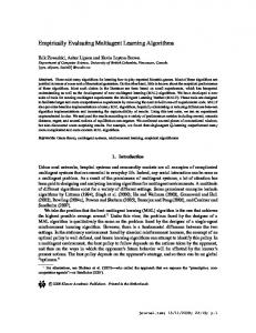
agent is defined by a communication radius; a link is created between two agents if the distance between them is less than this radius. An instance of this type of network is visible in Figure 2. We compute the communication radius such that the circular neigbhorhood will contain, on average, the correct number of agents to achieve the desired expected network density. This allows us to directly compare the results from the same expected network densities in both the random and proximity-based networks. We also considered one additional parameter, which was whether the networks are fixed or dynamic. In fixed networks agents always communicate with the same other agents each generation, i.e., the breeding neighborhoods for the genetic algorithm remain constant. In dynamic networks, agents may communicate with different agents every generation, i.e., the breeding neighborhoods change. These two factors together result in four network topologies that we will examine: (1) fixed proximity-based, (2) fixed random, (3) dynamic proximity-based, and (4) dynamic random. Proximity-based and random networks used different forms of dynamics. In dynamic proximity-based networks, agents move slowly (about 1% of the world’s diameter) forward across the world, turning randomly (up to 15 degrees right or left) each generation. Agents’ local neighborhoods update based on the agents currently within their communication radius. In dynamic random networks, a new network structure is generated each generation, using the same Erd˝ osR´enyi model as described above. These particular forms of dynamics are a subset of a larger class of dynamics. For example, instead of reassigning every link in the dynamic random networks we could change a smaller fraction of links each generation, and in the proximity-based networks, the rate and method of agent movement could be altered. We chose these two network topologies to be representative of two ends of a spectrum from unstructured (random) to structured (proximity-based) topologies. In future work, these networks topologies will act as base cases for comparison to other topologies. We were also interested in the effects of dynamics on networks, and examining these base cases assists in isolating the effects of dynamics from other complicating factors of network structure. We conducted two experiments with this model to investigate how the density affects the overall performance of the GA. All of the components of the model are implemented in NetLogo [16]. In all of the experiments described below, we will run the model with a different level of density until an optimum solution is found, and we measure how long it takes to find that optimum solution, or we give up if it takes more than 3000 generations3 .
4.
EXPERIMENT 1: NETWORK DENSITY
In the first experiment, we vary the network density from 0% to 100% at 5% increments, and examine all four network topologies. We also examine both the easy problem (100 bit hdf) and the harder problem (200 bit hdf). For each parameter set we ran the model sixty (60) times, and record the time until a perfect solution is found. We average the results, and present them for the easy problem in Figure 3 and for the harder problem in Figure 4.
4.1 3
Figure 1: Random Network with density of 0.01 after discovery of optimum. Agents are colored according to the fitness of the solution they possess. Higher luminance values indicate better solutions.
Figure 2: Proximity Network with density of 0.01 after discovery of optimum. Agents are colored according to the fitness of the solution they possess. Higher luminance values indicate better solutions.
Experiment 1 Results
Most runs find the optimum well before 3000 generations.
Electronic copy available at: http://ssrn.com/abstract=1846665
3000 fixed proximity dynamic proximity fixed random dynamic random
2500
generation perfect solution was found
generation perfect solution was found
3000
2000
1500
1000
500
0
2500
2000
1500
1000
500
0 0
20
40 60 network density (percentage)
80
100
Figure 3: Average time to optimum versus density from 0% to 100% for all four network topologies on the 100-bit hdf problem. Bars show standard error.
In the easier problem (Figure 3), it can be seen that all four topologies result in similar performance. In all four cases, as long as the network density is at or above 5%, the population is able to find solution in roughly the same amount of average time, around 250 generations. In the harder problem (Figure 4), a similar qualitative phenomenon can be observed. With a network density 5% or greater, the population is always able to find a solution somewhere between 1000 and 1500 generations. The results on this harder problem are less consistent than they are on the easier problem, and there is no discernible pattern as to when the topologies perform differently.
4.2
fixed proximity dynamic proximity fixed random dynamic random
Experiment 1 Discussion
Despite the lack of differences in the network topologies there are several interesting phenomenon to observe. First of all, the system is robust, even for sparse networks (≤ 5% density) it performs equivalent to 100% network density. This panmictic (all mixing) population is equivalent to global communication. These results indicate that there is no reason that every individual needs to be in communication with every other individual in the population. Instead, each individual needs to only communicate with a small local neighborhood, regardless of the interaction topology. It should also be noted that 0% network density is the same as every agent working alone. In this model, agents are only able to measure the performance of their solution indirectly, by comparing it to the performance of solutions of other agents they communicate with. Thus, agents operating alone wind up mutating bits at random. Values of network density between 0% and 100% reflect varying degrees of local communication. The results of these experiments illustrate that little local communication is necessary to achieve the same effects as global communication. Moreover, these results seem to hold independent of the difficulty of the problem. In applications, this might guide decision-making about the amount of effort that should be invested in inter-agent communication.
0
20
40 60 network density (percentage)
80
100
Figure 4: Average time to optimum versus density from 0% to 100% for all four network topologies on the 200-bit hdf problem. Bars show standard error.
5.
EXPERIMENT 2: A CLOSER LOOK
We designed a follow-up experiment to determine two things. First, at what network density (between 0% and 5%) does agent communication break down significantly enough that the group problem solving efficiency is diminished. Second, how do the different network topologies affect the performance of the system, given very low network densities. In this experiment, we varied the network density from 0% to 5% at 0.1% increments, and again examined results for all four network topologies on both the easier (100 bit hdf) and the harder (200 bit hdf) problems. For each parameter set we ran the model sixty (60) times, and recorded the time until a perfect solution is found. We averaged the results, and present them for the easy problem in Figure 5 and for the harder problem in Figure 6. Only network densities between 0% to 3% are shown, to highlight the region of interest. Additionally, we measured the diversity of the population’s solutions at the end of the run (3000 generations). Our diversity measure was the average pairwise Hamming distance between agents’ solutions (strings of bits), normalized to be between 0.0 (completely homogenous) and 1.0 (maximally diverse).4 We average the results of the 60 repetitions of the model, and present them for the easy problem in Figure 7 and for the harder problem in Figure 8.
5.1
Experiment 2 Results
In the easier problem (Figure 5), we now find a difference in the performances of the four topologies. The dynamic random structure requires the least amount of network density in order to achieve the same results as the panmictic population. After this, the dynamic proximity and fixed random structures have equivalent behavior. Finally, the fixed proximity structure has the worst performance of the four interaction topologies. However, in all four cases, as long as the network density is over 1.8%, the population is able to find a solution in roughly the same amount of average time, around 250 generations. 4
This is one of many possible diversity measures.
In the harder problem (Figure 6), a similar qualitative phenomenon can be observed. The dynamic random structure performs the best, with the fixed random and dynamic proximity structures coming in second, and the fixed proximity structures performing the worst. However, with a network density greater than 1.9%, the population is consistently able (on average) to find a solution somewhere between 1000 and 1500 generations regardless of the network structure. Again, the results on this harder problem are less consistent than they are on the easier problem, and there is no statistically significant pattern as to when the topologies perform differently after this 1.9%. The diversity plots (Figures 7 and 8), show that decreases in diversity occur in the same order as the decreases in time to optimal. As the expected network density increases, first the dynamic random network diversity decreases, then the fixed random and the dynamic proximity, with the fixed proximity having the slowest decrease in diversity. Moreover, these decreases in diversity occur at roughly the same network densities as the decreases in time to optimal. We ran additional experiments identical to this one, except with variations on the selection process (i.e., choosing the best of two (2) or four (4) solutions from the neighborhood, instead of three (3), or using “roulette” selection which chooses probabilistically from the whole local neighborhood proportional to each solution’s fitness). These experiments yielded the same qualitative results as those presented here.
5.2
Experiment 2 Discussion
There are several clear results from this data. First, dynamic topologies require less network density to achieve the same level of performance as do fixed topologies. Second, random topologies require less network density to achieve the same level of performance as do proximity-based topologies. Moreover, these results appear to be independent of the difficulty of the problem. Several hypotheses explain these results. First, proximitybased fixed topologies are still segmented at higher network densities than the other topologies. Since the network is defined by other agents within a certain local radius, at low levels of density it is common for not all of the agents to be connected to each other in one giant component. These isolated components cannot share information with each other, which prevents global coordination to collectively solve the problem. Dynamic topologies are not subject to this problem because they are constantly changing their network connections so isolated groups will eventually be connected to the rest of the group. The fixed random network topology is also less susceptible to this problem because the construction of the random networks means that neighbors of agents are not likely to be connected to other neighbors of the same agent, i.e., they have a low clustering coefficient. As a result, for fairly low network densities there is still a giant component connecting many of the agents. A second hypothesis is that the key ingredient to successful group problem solving is the ability for good solutions to propagate quickly through the whole population. One important measure for this on fixed networks is the average length of the path between any two nodes in the network (average path length). Random networks have a shorter average path length than proximity-based networks. In dynamic networks, average path length is not well-defined, but since agents are constantly changing their partners, the number of
generations it takes for an innovative idea to spread across the network should be smaller. A third hypothesis is similar to the second, but instead the emphasis is on the initial rapidity with which a solution can reach a reasonably broad audience. In particular, if the clustering coefficient of the network is too high, then agents will pass information to their neighbors, who will mostly pass among each other, rather than passing it to new agents that haven’t been exposed to it yet. Random networks have lower clustering coefficients than proximity-based networks. In the dynamic topologies, the clustering coefficient is not well-defined, but since agents are not exposed to the same individuals every generation, good information is more likely to initially spread more quickly. The diversity results support these hypotheses that the key to solving these problems is to have good communication across the network. High diversity indicates that there are pockets of the network that are not communicating well with other pockets of the network and thus have evolved their own different solutions to the problem. When a topology promotes quick communication of good ideas across the network then you would expect less diversity than when it takes more time for these partial good solutions to permeate. These results clearly indicate that random-network topologies outperform proximity-based network topologies, and that dynamic topologies outperform fixed topologies.
6.
CONCLUSIONS AND FUTURE WORK
We have presented a model of multi-agent learning that is embedded in a network context, and have discussed three main results. First, the system is robust (maintains optimal performance) for a large range of network densities (& 2%), but below a certain density threshold the performance decreases sharply (i.e., there is a phase transition). Second, this threshold is lower for the dynamic networks than for the fixed networks. Third, this threshold is lower for the random topology than the proximity topology. Beyond these specific research questions, our research has potential applications in three different disciplines: evolutionary computation (EC), social science, and agent-based modeling (ABM). From an EC perspective, the presented model is an investigation into the effect of various breeding networks in a GA. Such an investigation allows researchers interested in GAs to develop a new understanding of how breeding topologies affect the performance of the GA, and is directly relevant to researchers interested in the question of takeover time in GAs [8]. Within this field our findings supports the idea that panmictic populations are not necessary in order to achieve maximal performance in a GA. There may also be ways to use breeding topologies to increase the performance of a GA. Thus, these results may have applications in the design of robust distributed GAs. From a social science perspective, this model examines the diffusion of innovation in social networks. The agents can be viewed as individuals in an organization, where each individual is involved in the process that is called “reinvention” in the diffusion of innovation literature [11]. Reinvention is where innovations are modified by individuals in order to solve a new problem, or to solve an existing problem better. Our results indicate that little communication between individuals is necessary for reinvention to work. Long-range (i.e., cross-silo) communication is superior to proximity-based communication. Dynamic communication
3000 fixed proximity dynamic proximity fixed random dynamic random
generation perfect solution was found
2500
2000
1500
1000
500
0 0
0.5
1 1.5 2 network density (percentage)
2.5
3
Figure 5: Average time to optimum versus network density from 0% to 3% for all four network topologies on the 100-bit hdf problem. Standard error bars are shown.
3000 fixed proximity dynamic proximity fixed random dynamic random
generation perfect solution was found
2500
2000
1500
1000
500
0 0
0.5
1 1.5 2 network density (percentage)
2.5
3
Figure 6: Average time to optimum versus network density from 0% to 3% for all four network topologies on the 200-bit hdf problem. Standard error bars are shown.
population diversity (after 3000 generations)
1 fixed proximity dynamic proximity fixed random dynamic random 0.8
0.6
0.4
0.2
0 0
0.5
1 1.5 2 network density (percentage)
2.5
3
Figure 7: Average final solution diversity versus network density from 0% to 3% for all four network topologies on the 100-bit hdf problem. Standard error bars are shown (but may be too small to be discernable).
population diversity (after 3000 generations)
1 fixed proximity dynamic proximity fixed random dynamic random 0.8
0.6
0.4
0.2
0 0
0.5
1 1.5 2 network density (percentage)
2.5
3
Figure 8: Average final solution diversity versus network density from 0% to 3% for all four network topologies on the 200-bit hdf problem. Standard error bars are shown (but may be too small to be discernable).
networks are also beneficial; talking to different people everyday facilitates reinvention. From an ABM perspective, we consider how several types of agent interaction dynamics affect the exchange of information. This model can be viewed generally as a model of agent communication, and our results describe how levels of communication influence performance. This model provides researchers, who are interested in communication processes within ABMs, guidelines for what to expect based upon how their agents are distributed and how the agents communicate. For instance, for engineers interested in using a cloud of “smart-dust” to collectively solve difficult problems, our results recommend choices for communication topologies and connectivity requirements to achieve success. There are many additional questions that could be considered when examining this model. For instance, we speculated that dynamic topologies can more quickly distribute information across the network, and that they are exposed to a wider range of information quickly. However, as mentioned above, the average path lengths and clustering coefficients are not well-defined for dynamic networks and so the creation of dynamic or generalized versions of these measures might facilitate the understanding of how dynamic network structures affect performance of these systems. Another phenomena that warrants investigation is the role that particular nodes play in the system performance. Researchers interested in the diffusion of innovation would be particularly interested in this question. It has been speculated that “influential” nodes play a key role in the diffusion of innovation, though this role has recently been brought under speculation [15]. Influentials could be examined as highly connected nodes, or as nodes with special properties (e.g., nodes that only innovate and do not copy from other nodes), and this model provides a computationally tractable way of asking this question. We have also only investigated two classes of network structures (proximity and random) in this model. Additional topologies like small-world topologies [13] and scalefree networks [1] should be investigated. Since scale-free and small-world both maintain higher clustering coefficients than expected given their lower average path lengths, they may provide a way for agents in networks to gain the benefits of local communication, and long-distance communication at the same time. Evaluating performance on these networks would also help us diagnose the primary structural factors that contribute to stable multi-agent learning in our model. At very low network densities, how much is performance controlled by average path length as opposed to clustering coefficient? If we could answer this question, then we may be able to design better multi-agent learning systems. Besides changing the network parameters, we could also vary the GA parameters. For instance, we could examine the interaction between the mutation rate and the network structure. A high mutation rate allows for a greater probability of innovation, but it can also cause good solutions to be destroyed before spreading through the population. However, high network densities may lessen the negative effects of mutation by raising the rate of spreading, suggesting a trade-off between mutation rate and network density. There are many interesting questions that can be addressed by this model. In general, the goal of our research project is to take a step back from particular applications and build higher-level models that can be employed in a
wide variety of circumstances. By studying these “metamodels” we can provide advice, guidelines, and frameworks to researchers interested in a wide variety of fields. Acknowledgments: We thank the Northwestern Institute on Complex Systems for providing support for WR, and Luis Amaral for access to his Computing Cluster.
7.
REFERENCES
[1] Barabasi, A.-L. Linked: The New Science of Networks. Perseus Books Group, 2002. ˝ s, P., and Re ´nyi, A. On random graphs. i. [2] Erdo Publicationes Mathematicae 6 (1959), 290–7. [3] Giacobini, M., Tomassini, M., and Tettamanzi, A. Takeover time curves in random and small-world structured populations. Proceedings of the 2005 conference on Genetic and evolutionary computation (2005), 1333–1340. [4] Holland, J. Adaptation in Natural and Artificial Systems. University of Michigan Press, Ann Arbor, MI, 1975. [5] Holland, J. H. Building blocks, cohort genetic algorithms, and hyperplane-defined functions. Evolutionary Computation 8, 4 (2000), 373–391. [6] Mitchell, M., Forrest, S., and Holland, J. H. The royal road for genetic algorithms. In Proceedings of the First European Conference on Artificial Life, 1991 (Paris, 11–13 1992), F. J. Varela and P. Bourgine, Eds., The MIT Press, pp. 245–254. [7] Moody, J. The Importance of Relationship Timing for Diffusion. Social Forces 81, 1 (2002), 25–56. [8] Payne, J. L., and Eppstein, M. J. Takeover times on scale-free topologies. In GECCO ’07: Proceedings of the 9th annual conference on Genetic and evolutionary computation (New York, NY, USA, 2007), ACM, pp. 308–315. [9] Payne, J. L., and Eppstein, M. J. Using pair approximations to predict takeover dynamics in spatially structured populations. In GECCO ’07: Proceedings of the 2007 GECCO conference companion on Genetic and evolutionary computation (New York, NY, USA, 2007), ACM, pp. 2557–2564. [10] Rand, W., and Riolo, R. Shaky ladders, hyperplane-defined functions and genetic algorithms. In Evoworkshops (2005), F. Rothlauf et al., Eds., vol. 3449 of LNCS, Springer. [11] Rogers, E. M. Diffusion of Innovations, fifth ed. Free Press, 2003. [12] Tomassini, M. Spatially Structured Evolutionary Algorithms: Artificial Evolution in Space and Time. Springer, 2005. [13] Watts, D. J. Small Worlds: The Dynamics of Networks Between Order and Randomness. Princeton University Press, 1999. [14] Watts, D. J. A simple model of global cascades on random networks. Proceedings of the National Academy of Sciences 99, 9 (2002), 5766–5771. [15] Watts, D. J., and Dodds, P. S. Influentials, networks, and public opinion formation. Journal of Consumer Research 34, 4 (December 2007), 441–458. [16] Wilensky, U. NetLogo. Center for Connected Learning and Computer-based Modeling, Northwestern University, Evanston, IL, 1999.