Multi-Agent Negotiation using Combinatorial Auctions with ... - CiteSeerX

Multi-Agent Negotiation using Combinatorial Auctions with Precedence Constraints∗ John Collins†and Maria Gini University of Minnesota

Bamshad Mobasher DePaul University

Abstract We present a system for multi-agent contract negotiation, implemented as an auctionbased market architecture called MAGNET. A principal feature of MAGNET is support for negotiation of contracts based on temporal and precedence constraints. We propose using an extended combinatorial auction paradigm to support these negotiations. A critical component of the agent negotiation process in a MAGNET system is the ability of a customer to evaluate the bids of competing suppliers. Winner determination in standard combinatorial auctions is known to be difficult, and the problem is further complicated by the addition of temporal constraints and a requirement to complete the winner-determination process within a hard deadline. We introduce two approaches to the extended winner determination problem. One is based on Integer Programming, and the other is a flexible, multi-criterion, anytime bid evaluator based on a simulated annealing framework. We evaluate the performance of both approaches and show how performance data can be used in the agent’s deliberation-scheduling process. The results show that coarse problem-size metrics can be effectively used to predict winner-determination processing time.

1

Introduction

Recently, the complexity of logistics involved in manufacturing has been increasing nearly exponentially. Many processes are being outsourced to outside contractors, making supply chains longer and more convoluted. The increased complexity is often compounded by reduced inventories and accelerated production schedules which demand tight integration of processes across multiple self-interested organizations. Firms can cut costs and improve efficiency by moving online. Instead of fulfilling orders from warehouses, companies will look for partners that can provide coordinated components and services in order to meet consumers demand for make-to-order products. Thus, the field is ripe for the introduction ∗

This work was supported in part by the National Science Foundation, awards NSF/IIS-0084202 and NSF/EIA-9986042 † [email protected]

1

of systems that automate logistics planning among multiple entities such as manufacturers, part suppliers and specialized subcontractors. Current e-commerce systems typically rely on either fixed-price catalogs or simple auctions. Companies usually work with pre-qualified suppliers, and buyer-supplier relationships depend on factors such as quality, delivery performance, and flexibility, in addition to cost [14]. In addition, current e-commerce systems do not have any notion of time (except for domain specific systems such as SABRE used in the travel industry). Time plays a fundamental role in supply-chain formation and management, since many products are made up of different parts and require multiple suppliers who have to coordinate their work. We are interested in studying how a group of heterogeneous, self-interested agents, can make commitments and carry out plans that require multiple tasks and coordination among multiple agents. We have proposed a market architecture [9] and we have implemented prototypes of both the market architecture and the agents. We call this system MAGNET (Multi AGent NEgotiation Testbed). MAGNET provides support for multi-agent negotiations for tasks with temporal and precedence constraints. This is especially important for the coordination of supply-chain management with production scheduling. One of the more difficult problems an agent faces in dealing with negotiation over collections of tasks is the problem of evaluating bids. Since we use an auction mechanism to carry out the negotiation, the bid-taking agent must solve a combinatorial winner-determination problem. In our case, this requires satisfying temporal feasibility constraints while attempting to minimize cost. We have developed and tested an Integer Programming (IP) formulation of this problem, along with a highly tunable anytime search, based on a Simulated Annealing [23] (SA) framework. In a time-limited negotiation environment, both approaches have value. This paper is organized as follows: in Section 2 we identify the key requirements for agents and supporting infrastructure that can support time-limited negotiation over coordinated tasks, and we present a novel architecture that satisfies those requirements. Section 3 describes in more detail the decision processes that must be performed by the Customer agent, focusing primarily on the bid-evaluation process. Section 4 describes our hybrid approach to bid evaluation that appears to balance the requirements for anytime performance with the desire for optimal solutions. Section 5 presents the results of a set of experiments that attempt to characterize the winner determination search process. Section 6 relates our work to other published research. Finally, in Section 7, we conclude and discuss further research opportunities.

2

MAGNET Agents and their Environment

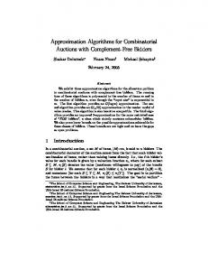
MAGNET gives an agent the ability to use market mechanisms (auctions, catalogs, timetables, etc.) to discover and commit resources needed to achieve its goals. We assume that agents are heterogeneous and self-interested, and may be acting on behalf of different individuals or commercial entities who have different goals and different notions of utility. Agents may fulfill one or both of two roles with respect to the MAGNET architecture, 2

as shown in Figure 1. Customer agents pursue their goals by formulating and presenting Requests for Quotations (RFQs) to Supplier agents through a market infrastructure [8]. The RFQ specifies a task network that includes task descriptions, a precedence network, and possibly other time constraints. Customer agents attempt to satisfy their goals for the least net cost, where cost factors can include not only bid prices, but also goal completion time and risk factors. More precisely, these agents are attempting to maximize the utility function of some user, as discussed in detail in [3].

Figure 1: The MAGNET architecture Supplier agents attempt to maximize the value of the resources under their control by submitting bids in response to those RFQs, specifying what tasks they are able to undertake, when they are available to perform those tasks, and at what price. Suppliers may submit multiple bids to specify different combinations of tasks, with prices and time constraints. Currently, MAGNET supports exclusive OR bids (if a supplier submits multiple bids, only one can be accepted), but other bid semantics are possible [19]. The MAGNET market infrastructure acts as an intermediary and information repository in support of participating agents. Most importantly, it serves an ontology of task types along with market statistics. These statistics include expected duration and variability, expected price and variability, resource availability, and lead time. The market also collects statistics on supplier reliability, which customer agents can use to estimate risk during the bid-evaluation process. As an example, let’s imagine we need to construct a garage, which must be completed before the first snowfall. Figure 2 shows a plan to complete the garage. Our plan is complicated by a couple of factors. The special doors must be ordered ahead, and will arrive one week after we order them. They also cannot be left outdoors, and so must be installed immediately when they arrive. Also, there is a housing boom in our area, and carpenters are hard to find on short notice. In this scenario, we expect that the template for the garage-building plan would come from a library of plan outlines, or it would be created manually. The specific task types with 3

Roofing Carpentry

Wiring Install Doors

Order Doors

End

Begin

Masonry

Figure 2: Plan for building a garage specifications and market statistics would be provided by a construction-services market server. The customer agent’s user would fill in specifics of the plan, adding necessary time constraints, adding details, and selecting options for the various tasks. The agent would then formulate an RFQ and present it to the market to request bid responses from suppliers. The level of user interactivity and the balance between user control and agent autonomy are likely to be quite variable among different application domains.

3

Activities of the Customer Agent

We now focus on the structure and responsibilities of a Customer agent in the MAGNET environment. As indicated in Figure 1, the basic operations are planning, bidding, and plan execution. For experimental purposes, we have implemented a simple Planner that generates random task networks with well-defined statistics, and a Bid Manager with a fairly rich set of tools for composing RFQ’s and selecting bids. We have also implemented a User Interface that allows manual creation and editing of plans, as well as monitoring and control of customer agent activities during the bid and execution cycles. The Execution Manager has not yet been implemented.

3.1

Task Networks

The Planner’s task is to turn the agent’s high-level goals into plans, represented as task networks. We have seen an example earlier in Figure 2. More formally, a task network P = (S, V) contains a set S of task descriptions, and a set V of precedence constraints. For each task s ∈ S, there is a possibly empty set v ∈ V of precedence constraints v = {s′ ∈ S | s′ ≺ s}, the set of tasks s′ whose completion must precede the start of task s. Other types of precedence constraints are certainly possible, such as start-start and finish-finish constraints. Notice that the task network itself need not be situated in time. That will happen when we compose the RFQ. Also notice that the operations in the task network do not need to be linearized with respect to time, since operations can be executed in parallel by multiple agents. The planner in the MAGNET testbed generates tasks by selecting randomly from a library of task types, and then creates random precedence constraints among them. It can also accept pre-defined plans, from a library or from a user interface. 4

The task network is a central data structure throughout a MAGNET system. The Bid Manager uses it to generate RFQs and to evaluate and record resource commitments and timing data, and the Execution Manager uses it to monitor and repair the ongoing execution of the plan. Part or all of the task network is included in a RFQ. In fact, each of the other components can be characterized by how it uses, decorates, extends, or updates the task network.

3.2

RFQ Generation

Plan completion

Start of execution

Bid Award deadline

Bid deadline

Send RFQ

Start planning

The Bid Manager is responsible for ensuring that resources are assigned to each of the tasks of a task network, that the assignments taken together form a feasible schedule, and that the cost of executing the plan is minimized. This cost must also be less than the value of the goal at the time the goal is reached. When the Bid Manager is invoked, some tasks in the task network may already be assigned. This can occur because the Execution Manager may use the Bid Manager to repair a partially-completed task network in which previously determined assignments have failed, because the agent will perform some of the tasks itself, or because bidding is being carried out in multiple stages. For example, I may decide to wire my new garage myself, and so I might not wish to solicit a contract for that task. Before constructing the RFQ, the Bid Manager must allocate time to negotiation and plan execution. The timeline in Figure 3 shows an abstract view of the progress of a single negotiation. At the beginning of the process, the Customer agent must allocate deliberation time for its own planning, for supplier bid preparation, and for its own bid evaluation process. Two of these time points, the Bid deadline and the Bid Award deadline, must be commumicated to suppliers as part of the RFQ. The Bid deadline is the latest time a supplier may submit a bid, and the Bid Award deadline is the earliest time a supplier may expire a bid. The interval between these two time points is available to the customer to determine the winners of the auction.

Customer deliberates Supplier deliberates

Figure 3: Typical Agent Interaction Timeline In general, it is expected that bid prices will be lower if suppliers have more time to prepare bids, more time, and more schedule flexibility in the execution phase. Minimizing the delay between the bid deadline and the award deadline will also minimize the supplier’s 5

opportunity cost. On the other hand, the Customer’s ability to find a good set of bids is dependent on the time allocated to bid evaluation. We are interested in the performance of the winner determination process precisely because we realize that it takes place within a window of time that must be determined ahead of time, and because we expect better overall results if we can maximize the amount of time available to suppliers while minimizing the time required for customer deliberation. These time intervals can be overlapped to some extent, but doing so creates opportunities for strategic manipulation of the Customer by the Suppliers, as discussed in [5]. The Bid Manager attempts to produce an RFQ that will solicit the most advantageous set of bids possible. It cannot evaluate bids that are not received, nor can it make successful combinations of bids that conflict with one another over precedence constraints. The approach we take is to find a balance between giving maximum flexibility to suppliers, ensuring that the resulting bids will combine feasibly, and ensuring that the job will be completed by the deadline. We do this by setting early-start and late-finish times in the RFQ for each task. More formally, an RFQ r = (Sr , Vr , Wr ) contains a subset Sr of the tasks in the task network P, with their precedence relations Vr , and time windows Wr specifying constraints on when each task may be started and completed. As pointed out earlier, there might be elements of the task network P that are not included in the RFQ. For each task s ∈ Sr in the RFQ the Bid Manager must specify: • a time window w ∈ Wr , consisting of an earliest start time tes (s, r) and a latest finish time tlf (s, r), and • a set of precedence relationships Vs = {s′ ∈ Sr | s′ ≺ s}, the set of other tasks s′ ∈ Sr whose completion must precede the start of s. There is no requirement that the bidding for a given task network be driven through a single RFQ, and there is no requirement that all precedence relationships be specified in the RFQ. The only requirement is that all specified precedence relationships be among tasks in a single RFQ. We assume the agent has general knowledge of normal durations of tasks. One of the roles of the MAGNET market infrastructure is to gather and publish statistical information about duration and variability for the different task types, information about resource availability, and about the number of vendors who are likely to bid on each type of task. In order to minimize bid prices while minimizing the overall duration of the task network, the Customer agent schedules tasks ahead of time using expected durations. One straightforward way to do this is to compute early start and late finish times using the Critical Path (CPM) algorithm [15]. The Critical Path algorithm walks the directed graph of tasks and precedence constraints, forward from time t0 to compute the earliest start tes (s) and finish tef (s) times for each task s ∈ S, and then backward from time tgoal to compute the latest finish tlf (s) and start tls (s) times for each task. The minimum duration of the entire task network, defined as max(tef (s)) − t0 , is called the makespan of the task network. The difference between tgoal 6

and the latest early finish time is called the total slack of the task network. If tgoal is set equal to t0 + makespan, then the total slack is 0, and all tasks for which tef (s) = tlf (s) are called critical tasks. Paths in the graph through critical tasks are called critical paths. The tradeoff between minimizing task duration and attracting usable bids from suppliers affects how slack should be set. Our method based on CPM can work if adequate approximations of task durations are known, because it will reduce the likelihood of bids being rejected for failure to mesh with the overall schedule, and it will reduce the average bid prices to the extent that it reduces speculative resource commitments on the part of suppliers. It is clearly not optimal, however. Intuitively, this is because the CPM blindly method allocates the additional time to all tasks. Non-critical tasks (tasks not on the critical path) are often allocated too much time, causing unnecessary overlap in their time windows. Also, no distinction is made between tasks for which large numbers of potential bidders exist, and tasks that are likely to interest only a few bidders. The optimal setting of RFQ time windows would require detailed knowledge of factors such as likely numbers of bidders and the likely constraint tightness on the resources needed to carry out the tasks. Since the Customer agent cannot know this data precisely, the agent must use approximations. The Market maintains statistics to support this, but there is clearly more work to be done in this area. For our garage-building scenario, an RFQ might look like Figure 4. It includes all tasks in the task network, along with their precedence constraints. The time windows, however, need not obey the precedence constraints; the only requirement is that the accepted bids obey them. The reason for doing this is to make the RFQ more attractive to suppliers, on the assumption that a supplier is more likely to bid, and likely to submit a lower-cost bid, if it is given greater flexibility in scheduling its resources. This complicates the problem of evaluating bids, as we shall see. Masonry Carpentry Roofing Order Doors Install Doors 0

1

2

3

4

5

week

Figure 4: RFQ Example Many variations on this example are possible. Time windows can be set to avoid any overlap. This guarantees plan feasibility, since every bid will have to fit into a time window and the time windows guarantee the precedence constraints. This in turn will simplify the winner determination process. The disadvantage is a reduction of flexibility for suppliers, since time windows will generally be shorter, or an increase in the time needed to complete the tasks. 7

An alternative solution is to split the tasks into multiple RFQ’s. In our garage example, we might wish to defer requesting bids on the roofing, doors, and door installation until we have bids in hand for the carpentry. If we receive an unexpectedly early bid for the carpentry work, that would allow us to finish the job earlier than if we had built a single schedule, such as the one in Figure 4, with ample slack available to accommodate the expected shortage of carpentry resource availability.

4

Evaluating Bids

Each bid represents an offer to execute some subset of the tasks specified in the RFQ, for a specified price, within specified time windows. Formally, a bid b = (r, Sb , Wb , cb ) consists of a subset Sb ∈ Sr of the tasks specified in the corresponding RFQ r, a set of time windows Wb , and an overall cost cb . Each time window ws ∈ Wb consists of an earliest start time tes (s, b), a latest finish time tlf (s, b), and a task duration d(s, b). It is a requirement of the protocol that the time window parameters in a bid b are within the time windows specified in the RFQ, or tes (s, b) ≥ tes (s, r) and tlf (s, b) ≤ tlf (s, r) for a given task s and RFQ r. This requirement may be relaxed, although it is not clear why a supplier agent would want to expose resource availability information beyond that required to respond to a particular bid. A solution to the bid-evaluation problem is defined as a complete mapping S → B of tasks to bids in which each task in the corresponding RFQ is mapped to exactly one bid, and that is consistent with the temporal and precedence constraints on the tasks as expressed in the RFQ and the mapped bids. Figure 5 shows a very small example of the problem the Bid Evaluator must solve. As noted before, there is scant availability of carpentry resources, so we have provided an ample time window for that activity. At the same time, we have allowed some overlap between the Carpentry and Roofing tasks, perhaps because we believed this would attract a large number of bidders with a wide variation in lead times and lower prices. Bid 2 indicates this carpenter could start as early as the beginning of week 3, would take 3 days, and needs to finish by the end of week 3. The lowest-cost bid for roofing is Bid 3, but we clearly can’t use that bid with Bid 2. The lowest-cost complete, feasible combination for these three tasks is Bids 1, 2, and 5. The winner determination problem for combinatorial auctions has been shown to be N P-complete and inapproximable [26]. This result clearly applies to the MAGNET winner determination problem, since we simply apply an additional set of (temporal) constraints to the basic combinatorial auction problem, and we don’t allow free disposal. Because there can be no polynomial-time solution, nor even a polynomial-time bounded approximation, we must accept exponential complexity. We will see in Section 5 that we can determine probability distributions for search time, based on problem size metrics, and we can use those empirically-determined distributions in our deliberation scheduling process. A MAGNET Bid Evaluator is a search engine that takes a task network and a set of bids, and attempts to find an optimal or near-optimal complete mapping of tasks to bids, 8

Masonry Carpentry Roofing

RFQ 0

1

2

3

4

5

week

Bid1 Masonry: 500$ Bid2

Carpentry: 800$

Bid3

Roofing: 750$

Bid4

Carpentry: 1000$

Bid5

Roofing: 900$

Figure 5: Bid Example respecting temporal constraints. It must do this within the period of time allocated by the Process Planner, which may have been subdivided by the Bid Scheduler. We have implemented two evaluators: one uses an Integer Programming solver, and the other is a highly modular Simulated Annealing (SA) search engine [6]. We discuss each of them in turn.

4.1

Integer Programming approach

The Integer Programming (IP) solver operates in two phases. The first phase generates basic bid-compatibility constraints, and then walks all paths of length 2 or greater in the precedence network, across all compatible bid combinations, comparing time windows to discover feasibility constraint violations. The second phase composes an IP problem from the resulting constraints and passes the resulting matrix off to an external IP solver1 . This approach is somewhat different from the “standard” IP formulation for combinatorial auctions (see for example [1]), for two reasons. First, in the MAGNET domain we cannot use the “free disposal assumption” which states that unsold goods can be disposed of freely. In the MAGNET environment, all tasks must be allocated to bids in order to successfully complete the plan. Second, the temporal feasibility constraints dominate the formulation; without preprocessing, relatively small problems can easily generate 105 constraints. Proprocessing typically reduces the problem size by 2-3 orders of magnitude. To describe our IP formulation, we enumerate the set Sr of tasks in RFQ r as sj , j = 1..m. Each task sj has a precedence set Vj = {sj ′ |sj ′ ≺ sj }, the set of tasks sj ′ ∈ Sr that must be completed before sj starts. At the conclusion of the bidding process, we have a set B of bids bi , i = 1..n. We use 0/1 integer variables xi , i = 1..n to denote whether the corresponding bids bi are included in the result. 1

For our experiments, we used lp solve, available from ftp://ftp.ics.ele.tue.nl/pub/lp solve/

9

Preprocessing starts by discovering uncovered tasks and “singleton” bids. An uncovered task is simply a task sj that is not included in the task set Si of any bid bi ∈ B. If an uncovered task exists, then no solution is possible. If there is any task sj for which only one bid bi has been received we call bid bi a “singleton” bid. Any singleton bid bi must be part of any complete solution, and any bids bk that conflict with bi can then be discarded. In more formal terms, ∀j|

X i|sj ∈Si

1 = 1, xi = 1, ∀k|Si ∩ Sk 6= ∅, xk = 0

This test is repeated until no further singleton bids are detected. If any task becomes uncovered during this process, then no solution exists. We then discover conflict sets among the remaining bids. For each bid bi , its conflict set Ci is defined as the set of bids bi′ whose task sets overlap the task set of bi , i.e. Ci = ∀bi′ ∈ (B − bi )|Si′ ∩ Si 6= ∅ Clearly, only a single bid from any conflict set can be included in any solution. The final preprocessing step converts precedence relations among tasks to compatibility constraints among bids. For each bid bi we walk the task precedence network Vr to discover whether the time windows specified for other bids bi′ are compatible with the time windows specified for bi . Each conflicting time window results in an infeasible bid combination g. Infeasible combinations may be of any length n = 2 . . . k where k is the maximum depth of the precedence network. They are defined as: G2 = ∀(bi ∈ B, bi′ ∈ (B − Ci ))|{sj ∈ Si , sj ′ ∈ (Vj ∩ Si′ ) |tls (sj , bi ) < (tes (sj ′ , bi′ ) + d(sj ′ , bi′ ))} G3 = ∀(bi ∈ B, bi′ ∈ (B − Ci ), bi′′ ∈ (B − Ci )) |{sj ∈ Si , sj ′ ∈ (Vj ∩ Si′ ), sj ′′ ∈ (Vj ′ ∩ Si′′ ) |tls (sj , bi ) < (tes (sj ′′ , bi′′ ) + d(sj ′′ , bi′′ ) + d(sj ′ , bi′ ))} .. . The IP formulation is then Minimize:

n X

c i xi

i=1

Subject to: • Bid selection – each bid is either selected or not selected. These are the integer variables that make this an integer programming problem. xi ∈ {0, 1} 10

• Coverage – each task sj must be included exactly once. This is an encoding of the coverage conflict sets discussed above. ∀j = 1..m

X

xi = 1

i|sj ∈Si

Note that under the free disposal assumption, each task would be included at most once, rather than exactly once. • Feasibility – The final preprocessing step described above produces sets Gn of bids that cannot be combined feasibly. We must specify that none of these sets can be entirely included in any solution. ∀n∀gn,m ∈ Gn ,

X

xi < n

i|bi ∈gn,m

More detail on this formulation is available in [4].

4.2

Simulated Annealing approach

A high level algorithm for our Simulated Annealing winner determination search is depicted in Figure 6. We use a basic simulated-annealing framework [23], with a finite queue (maximum length is beam width) and a number of enhancements to minimize wasted effort. Many complications are omitted, such as the fact that expand node (see Figure 8) may fail to produce a node. This can happen, for example, because the selected bid has already been tried against the selected node, or because of an optional uniqueness test. The simulated-annealing framework is a queue-based search, characterized by two elements, the annealing temperature T which is periodically reduced by a factor ε, and the stochastic node-selection procedure shown in Figure 7. Stopping conditions include a time limit and “patience factor” as shown in Figure 6, as well as empty queue. The patience factor is simply the number of nodes that have been generated without finding an improved evaluation score. It is typically a function of the problem size, but also may be a function of the number of nodes generated prior to the latest improved score. The queue can become empty if an optional feature is used that keeps track of the bids that have been used to expand the node in the past; when all bids that do not conflict with bids already in the node (where “conflict” can include the conflict sets and feasible bid combinations found for the IP solver) have been tried, the node is removed from the queue. This greatly reduces redundant effort in the search at the cost of keeping track of the remaining compatible bid set per node. Although this is a somewhat unorthodox approach for a stochastic search, it has proven to be very valuable in our situation because of the high cost of node evaluation. When a stopping condition other than time limit occurs, an optional restart protocol can be used. In most cases, search time is better spent running several shorter searches, rather than a single long search. We shall see an example of this in Section 5. 11

Procedure simulated annealing Inputs: S, V: the task network to be assigned B: the set of bids N0 : initial node, containing mapping of tasks to singleton bids Output: Nbest : the node having a mapping M(Nbest ) = S → B of tasks to bids with the best known evaluation Process: Q ← priority queue of maximum length beam width, sorted by node evaluation v(N ) v(N0 ) ← evaluate node(N0 ) /* see narrative in this section */ Nbest ← N0 /* initialize the result */ insert(Q, N0 ) /* insert the first node into the queue */ T ← T0 /* set the initial annealing temperature */ R ← current time Z ← 0 /* initialize the improvement counter */ while (¬empty(Q) ∧ R < time limit) ∧ (Z < patience) do N ← select node(Q, T ) /* see Figure 7 */ B ← select bid(N, B) N ′ ← expand node(N, B) /* see Figure 8 */ v(N ′ ) ← evaluate node(N ′ ) /* see narrative in this section */ insert(Q, N ′ ) if v(N ′ ) < v(Nbest ) then Nbest ← N ′ Z←0 else Z ←Z +1 T ← T (1 − ε) /* the value ε is the annealing rate */ return Nbest

Figure 6: Simulated Annealing algorithm for winner determination.

12

Procedure select node Inputs: Q: the current node queue, sorted so that v(Qn ) ≤ v(Qn+1 ) /* v(Qn ) is the evaluation of the nth node in Q */ T : the current annealing temperature 0 ≤ T ≤ 1 Output: Nnext : the selected node Process: r ← random(0, 1) /* a random number uniformly distributed between 0 and 1 */ R ← v(Q0 ) − T ln(1 − r)(v(Qlast ) − v(Q0 )) /* R is called the “target evaluation” */ /* Q0 and Qlast are the first and last nodes in the queue, respectively */ n←0 while v(Qn+1 ) ≤ R do /* find the last node whose evaluation is less than or equal to the target */ n←n+1 return Qn

Figure 7: The node-selection algorithm. Bid selection is done by a plug-in component that can be configured in a number of ways. The simplest selector simply makes a random choice among bids that are not part of the current mapping, and that are compatible with the bids currently mapped in the node. Others may focus on improving coverage, feasibility, or cost. Extensive experimentation has failed to show that any more informed method performs consistently better than a simple random approach. Node expansion (see Figure 8) is done by adding mappings of the selected bid to all the tasks covered by that bid, discarding mappings of any other bids that overlap the new bid. This will fail if the selected bid has already been used to expand the selected node, or because the bid was used to produce the current node. Not shown is the fact that expansion can also fail if an attempt is made to unmap a singleton bid (a bid that provides the only possible mapping for some task). Of course, no bids will ever be unmapped if we filter bid selections with the conflict sets Ci . Node evaluation produces a value v(N ) for node N which is a weighted sum of the following four factors: • coverage: are all the tasks covered? a bid that covers some not yet covered tasks should be preferred over a bid that covers tasks already covered. • feasibility: is the current partial solution feasible? If the Critical Path algorithm finds any negative slack, the current partial solution is not feasible, since it violates some time constraint. 13

Procedure expand node Inputs: N : the node to be expanded B: the bid to be added to M(N ), the bid-task mapping of N Output: N ′ : a new node with a mapping that includes B, or null if the mapping fails Process: W if (B ∈ BM(N ) ) (B ∈ tried (N )) then return null /* B is already in mapping of N, or as been tried previously. */ N ′ ← copy(N ) insert(tried (N ′ ), B) /* tried is a set */ T S ′ ← SB SM(N ′ ) /* S ′ is the set of tasks in both B and N’.M */ B ′ ← b ∈ BM(N ′ ) such that Sb ⊂ S ′ /* B ′ is the set of bids in M(N ′ ) whose tasks overlap the tasks in B */ ′ ∀b ∈ B , ∀s ∈ Sb , M(N ′ ) ← M(N ′ ) − m(s, b) /* remove mappings for B ′ */ ∀s ∈ SB , M(N ′ ) ← M(N ′ ) + m(s, B) /* add the mappings for B */ return N ′

Figure 8: The node-expansion algorithm. • cost: what is the total cost?

5

Experimental Results

Bid evaluation to determine winning bids is a critical part of the Customer agent’s behavior, and it is clearly a costly combinatorial problem. We have evaluated many approaches to building a search engine that performs well. It is important to characterize its performance because of the need to allocate time to it in the context of the overall negotiation process, and because failure to produce a result within the allocated time will result in failure of the negotiation. Our goal will be to find the probability distributions of search time based on easily-measured problem metrics. We prefer metrics that can be estimated prior to issuing an RFQ, since that is when deliberation scheduling must be done. This will allow us to schedule the winner-determination deliberation with a known level of confidence in finding a solution. We report on a set of experiments that give us the necessary probability distribution data for both the IP and SA approaches. There are clearly limits on scalability, and there will be unpredictable situations where good solutions will not be found within any fixed time limit.

14

5.1

Experimental Setup

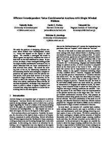
The experimental setup consists of a set of randomly-generated task networks, a set of randomly-generated bids for each task network, and a bid evaluator. The bid evaluation process is instrumented to measure both elapsed time and the number of steps performed (equation count for the IP evaluator, node count for the SA evaluator). All experiments were run using a dedicated 1800 MHz Linux machine. Timings are given in wall-clock time. The MAGNET system (including the IP preprocessor and the Simulated Annealing solver) is written in Java, and the IP solver is lp solve, written in C and available from ftp://ftp.ics.ele.tue.nl/pub/lp solve/. 5.1.1

Customer Agent: Construct and Issue a Request for Quotes

For these experiments, plans are randomly-generated task networks, with a number of controllable parameters, and the RFQs have a controllable amount of added slack. This slack is intended to give bidders enough flexibility to allow a significant fraction of them to bid. In these experiments, approximately 90% of bidders were able to bid on at least one task. Task Network variables include: 1. Number of tasks. 2. Mix of task types. Task types are characterized by average duration, duration variability, average price, and price variability. Both duration and price are normally distributed, positive values. 3. Branch factor. This is the average number of precedence relationships per task. For example, if a particular task has one predecessor and one successor, then the branch factor for that task is 2. Figure 9 shows the task network for the first of the problems used in the bid-count test series described in Section 5.2.2 below. S0

S16

S18 S4

S15

S11

S1

S12 S2 S13

S19

S10 S8

S9

S2 S6

S17 S7

S3 S5

S14

Figure 9: Task network for Problem #1. Box widths indicate relative task durations.

15

Before issuing the RFQ, we compute the makespan for the entire task network, and expected early start times tes (s) and late finish times tlf (s) for each task in the network, as specified in Section 3.2. RFQ variables include: 1. Total slack. This is the ratio (tgoal − t0 )/makespan of the time allowed for task network completion to the expected makespan of the task network. 2. Additional slack obtained by reducing task durations below their expected values. For these experiments, we simply multiplied each expected duration by a factor of 0.8 and re-ran the CPM algorithm. The only justification for this number is that it was the greatest reduction we found that did not cause most problems to have no feasible solutions. 5.1.2

Supplier Agent: Generate Bids

For these experiments, we used a test agent that masquerades as an entire community of suppliers. Each time a new RFQ is announced by the Market, the supplier attempts to generate a specified number of bids. For a given RFQ r, each bid bj is generated by selecting a task si at random from Sr , using the task-type parameters to generate a supplier time window wi (bj ) = (tes (si , bj ), tlf (si , bj ), d(si , bj ) for the task, and testing this time window against the time window wi (r) for task si in the RFQ. If the supplier’s time window wi (bj ) is contained within the RFQ time window wi (r), then we call this a “valid task specification” and add the task and its time window to the bid. If a valid task specification was generated, then with some probability, each predecessor and successor link from task si is followed to choose an additional task to add to the bid, and so on recursively. The resulting bids specify “contiguous” sets of tasks, and are guaranteed to be internally feasible. Finally, a cost is determined for the overall bid. Because valid task specifications are not always achieved, some attempts to generate bids will fail. Task durations are normally distributed around the expected value used by the Customer, and the time windows are randomly set to be smaller than the time windows specified in the RFQ and larger than the computed durations. Full details on the bid generation process are given in [7].

5.2

IP performance

In this section, and in the following section on SA performance, we attempt to characterize performance along 3 dimensions of problem size: (1) number of tasks in the task network, (2) number of bids submitted, and (3) the sizes of the submitted bids, i.e. the number of tasks per bid. Each problem set consists of 100 problems, with randomly-generated plans and randomly-generated bids as described above. Our problem generator has a large number of parameters; we kept all of them constant except for Task Count, Bid Count, and Bid Size.

16

5.2.1

Varying task network size

The first set of experiments examines scalability of the search process as the number of tasks varies, with a (nearly) constant ratio of bids to tasks (the ratio varies somewhat due to the random nature of the bid-generation process). Table 1 shows problem characteristics for this set. Each row in the table shows results for 100 problems. In the table, the “Bid Size” column gives the average size of bids (number of tasks per bid). The ratio of Task Count to Bid Size varies a bit because of the way bids are generated: Bid Size is more closely related to the depth of the precedence network than to Task Count. The “Solved” column gives the number of problems solved out of 100 (not all 100 problems were solvable), “Rows” gives the number of constraints in the generated IP problem, “Mean Time” gives the mean search time in milliseconds, including both preprocessor time and time spent in the IP solver itself, and σ gives the standard deviation of the “Total Time” column. Table 1: Task count experiment for the IP solver Task Bid Bid Count Count Size 5 13.5 2.1 10 29.0 3.3 15 45.4 4.5 20 61.0 5.4 25 77.7 6.3 30 93.4 7.4 35 110.6 8.4

# Solved Mean (of 100) Rows Time (ms) σ 94 19.9 16 7 94 46.3 41 24 90 84.0 111 90 85 153 235 172 85 287 565 633 80 496 986 859 73 774 2057 2057

While the data in Table 1 show average performance and give some indication of variability, we are really more interested in knowing the probability that a solution can be determined in a given amount of time. For that purpose, we show in Figure 10 the complete runtime distributions for four of the problem sets. For each curve, we show actual observations along with a lognormal distribution that minimizes the χ2 metric2 . Typical χ2 values range from 0.3 to 3.0 for 9 degrees of freedom, a good match. Note that the first parameter of the lognormal distribution is equal to the median value, which is significantly smaller than the mean for all sets. The value of data such as this is that we can now make decisions about time allocation with a specific degree of confidence. For example, we can say that for a problem the size of our 35-task, 123-bid sample, we have a 95% confidence in finding a solution using the IP solver in less than 5.6 seconds. In order to make use of this sort of data in an agent 2

The χ2 metric is determined by dividing the inferred density function into a number of equal areas, and counting the number of observations that fall into each of those zones. The χ2 value is the mean square deviation from a “perfect fit”.

17

1 0.9

Cumulative Probability

0.8 0.7 0.6 0.5 0.4 5 tasks logN(14.8,0.11) 15 tasks logN(91.3,0.33) 25 tasks logN(405.9,0.65) 35 tasks logN(1330.3,0.76)

0.3 0.2 0.1 0 1e+00

1e+01

1e+02 1e+03 1e+04 PreProcess + IP Search time (msec)

1e+05

Figure 10: Observed and inferred runtime distributions for the IP solver across a range of task count values, with a nearly constant ratio of bids to tasks. environment, we need to know how runtime scales along at least 3 dimensions of problem size: task count, bid count, and bid size. We have shown the task count data, but the results are necessarily conflated with variations in bid-size and bid-count. We’ll return to this after we have seen the bid count and bid size data. 5.2.2

Varying the number of bids

The next series examines the scalability of the IP method as the number of bids is varied over a 4:1 range, with task count and bid size held constant. Each row in Table 2 represents 100 problems, each with 20 tasks and varying numbers of bids. The same set of 100 task networks is used in each row; only the bid sets are varied. It is clear that the mean time scales exponentially with bid count; deviations in mean time and the lower variability at the low end of the range are likely the result of fixed overhead. In Figure 11, we see the measured and inferred probability distributions for five of the problems from Table 2. Again, we find good correspondence (0.2 < χ2 < 3.0, 9 dof) between the measured data and the inferred lognormal distributions. 5.2.3

Varying the sizes of bids

We now turn to the bid-size dimension. Our problem generator uses a somewhat inexact method to “influence” the sizes of bids. As described earlier, the bid-generation process generates “contiguous” bids by choosing a starting point in the task network, and then 18

Table 2: Bid Count experiment for the IP solver Task Bid Bid # Solved Count Count Size (of 100) 20 51.7 7.36 75 20 69.6 7.32 95 20 86.5 7.30 94 20 104.4 7.35 96 20 121.0 7.29 98 20 139.2 7.26 100 20 156.4 7.29 99 20 173.2 7.30 100 20 190.9 7.37 100 20 207.4 7.32 100

1 0.9


0.8 0.7

Mean Rows Time (ms) σ 92.2 109 61 125 185 95 193 335 228 284 501 452 583 1160 1820 782 1750 1970 1078 3060 3810 1691 4500 4220 2342 8300 15,000 3284 11,800 15,500

70 bids logN(163.4,0.26) 104 bids logN(398.5,0.44) 139 bids logN(1197.8,0.71) 173 bids logN(2964.8,0.96) 207 bids logN(6293.2,1.35)

0.6 0.5 0.4 0.3 0.2 0.1 0 1e+01

1e+02

1e+03 1e+04 PreProcess + IP Search time (msec)

1e+05

Figure 11: Observed and inferred runtime distributions for IP search for a range of bid count values, with task count = 20, and bid size ≈ 7.3. recursively following predecessor and successor links with some probability. In this series, we have varied that probability from a low of 0.2 to a high of 0.9. Bid size is also influenced by the sizes of time windows, since the “success” in generating a bid for a particular task is a function of both the size of the time window specified in the RFQ, and the simulated “resource availability” recorded for the type of each task. As shown in Table 3, the resulting 19

bid size varies from a low of 1.6 tasks/bid to 7.9 tasks/bid. Note the extreme difficulty and high variability of the 1.6 tasks/bid set. The task networks in these problem sets are the same as the ones used in the bid-count experiment. Table 3: Bid Size experiment for the IP solver Task Bid Bid # Solved Count Count Size (of 100) Rows 20 87.0 1.61 81 8430 20 86.6 2.20 92 2440 20 86.7 3.04 82 1760 20 86.5 4.22 99 781 20 86.6 5.42 96 374 20 86.9 6.40 96 259 20 86.5 7.30 94 193 20 86.6 7.90 94 164

Mean Time (ms) σ 87,300 334,000 7550 12,500 5550 13,700 1951 2710 740 607 466 365 345 250 285 199

Figure 12 shows the runtime observations and inferred distributions for four of the problems from Table 3. It appears that bid size variation affects the variability of solution time as much as it affects the mean time. 1 0.9


0.8 0.7 0.6 0.5 0.4 0.3

bid size = 1.61 logN(3598.0,5.52) bid size = 3.04 logN(1522.3,2.45) bid size = 5.42 logN(561.4,0.57) bid size = 7.90 logN(239.6,0.32)

0.2 0.1 0 1e+01

1e+02

1e+03 1e+04 1e+05 PreProcess + IP Search time (msec)

1e+06

1e+07

Figure 12: Observed and inferred runtime distributions for IP search for a range of bid size values, with task count = 20, and bid count ≈ 87. 20

5.2.4

Predicting IP runtime

We now have the necessary data to estimate the time that must be allocated to the winner determination process using the IP solver. The process is to choose a desired “probability of success”, and then to estimate parameters for a function that reasonably matches the inferred distributions at that level of probability. For example, in the left plot in Figure 13, we show a the 95, 50, and 5 percentile points from the inferred distributions from the bidcount experiment. The overlaid curve is 65.86 · 20.045x , which yields a root mean square error √ ǫ¯2 of 376 msec. In the right plot, we show the 95, 50, and 5 percentile points from the bid-size experiment. The overlaid curve in the right plot is 3.75 × 105 · 2−1.29x , which yields √ a ǫ¯2 of 8.2 sec. It seems likely that actual relationship between bid size and run time is more complex than the simple exponential relationship shown here. 1e+06

1e+05

95 percentile 50 percentile 5 percentile 3.75e5 * 2^(-1.29 x)

Total search time (msec)


1e+05 1e+04

1e+03

1e+02

40

60

80

100

120 140 Bid Count

160

180

1e+03

1e+02

95 percentile 50 percentile 5 percentile 65.86 * 2^(0.045 x)

1e+01

1e+04

1e+01 200

220

1

2

3

4 5 Bid Size

6

7

8

Figure 13: Estimating the time required to achieve 95% success rate using the IP solver for 20-task problems across a range of bid counts (left) and bid sizes (right). Finally, in Figure 14, we show an attempt to approximate a predictor for the search time required for the task-count experiment as detailed in Table 1. In addition to varying the task count, this experiment varies the bid count and the ratio of bid size to task count. We have taken the coefficients derived for bid count and bid size from above, and derived a coefficient for task count that minimizes ǫ¯2 . The derived formula is bs

runtime = 13.30 · 2(−25.8 tc +0.045bc+0.00384tc)

√ where tc is the task count, bc is the bid count, and bs is the bid size. The error ǫ¯2 for these coefficients is 71.5 msec. The search times on the 5-task set are so short they are very likely to have a large fixed overhead component (the lp solve process was re-started for each search). They almost certainly also suffer from the limited resolution of the system clock.

5.3

Characterizing the SA evaluator

Since the Simulated Annealing solver is a stochastic algorithm, we are interested in two types of performance data. The first is the same type of data that we saw for the IP solver in 21


1e+04

1e+03

1e+02

1e+01 95 percentile 50 percentile 5 percentile 13.30 * 2^(-25.8 bs/tc + .045 bc + .00384 tc)

1e+00 5

10

15

20 Task Count

25

30

35

Figure 14: Estimating IP search time for the task count experiment. the last section: performance across a range of task counts, bid counts, and bid sizes. The second is a more detailed look at the variability observed on individual problems. 5.3.1

Varying task network size

In Table 4 we report data on SA performance as task count varies. This is the same set of problems that was reported in Table 1 on IP performance, so bid count and bid size data can be read from that table. As before, we generated 100 problems in each set, and ran the IP solver to find the optimal solution (or to determine that the problem could not be solved). For each “solvable” problem we then ran the SA solver 20 times with different random number sequences, and captured time and node count data when the solver first found solutions with evaluations within 5% of the optimal value, within 1% of optimal, and equal to the optimal value found by the IP solver. In the remainder of this section, we’ll call these “5% solutions,” “1% solutions,” and “optimal solutions,” respectively. We then averaged the values for successful attempts on each problem, and we show here the statistics for those average values across the various problem sets. In Table 4, the “Failure Rate” column gives the proportion of attempts in which the SA solver failed to find optimal solutions to solvable problems (problems solved by the IP solver). The “Node Time” column reports the mean time per search node generated. These times grow as problem size increases because of the cost of maintaining the sorted search queue. Then we give Mean, Median, and Standard Deviation data for the time in milliseconds required to find a 5% solution and an optimal solution. We give both Mean and Median here because they are substantially different, due to the skewed distribution. Figure 15 shows graphically the observed distributions for 4 of the problem sets shown in Table 4. Each individual data point represents the average time required to find an optimal solution using the SA solver. Only the successful trials were included, so there is likely some truncation at the upper end of the range on the larger problems. We also show the closest 22

Table 4: Task count experiment for the SA solver Failure Node 5% Solution Rate Time Mean Median (%) (ms) (ms) (ms) σ 0 0.23 5 4 4 0 0.31 92 75 82 2 0.36 392 282 442 4 0.42 2000 857 4400 11 0.48 9420 2420 20,300 19 0.54 19,600 4270 45,600 23 0.60 35,700 8220 72,500

Task Count 5 10 15 20 25 30 35

Optimal Solution Mean Median (ms) (ms) σ 7 5 5 250 116 915 2270 652 7610 12,600 2550 29,500 26,500 6610 41,300 50,800 11,300 93,800 97,900 27,900 126,000

lognormal curves, but clearly the data is not as well-behaved as the IP data, and doesn’t fit a lognormal distribution for the larger problems. 1 0.9


0.8 0.7 0.6 0.5 0.4 0.3

5 tasks LN(5.3,0.59) 15 tasks LN(651.8,1.67) 25 tasks LN(6613.5,3.25) 35 tasks LN(27865.0,3.43)

0.2 0.1 0 1e-01

1e+00

1e+01

1e+02 1e+03 1e+04 SA Search Time (msec)

1e+05

1e+06

1e+07

Figure 15: Observed and lognormal runtime distributions for SA search to find optimal solutions across a range of task count values. In a time-limited negotiation situation, we might be willing to settle for a solution that is less than optimal. An obvious question is how much time we gain by doing so. Figure 16 shows the detailed aggregate behavior for two of the problem sets in Table 4. Again, each point represents the mean time required to find solutions to the indicated level of accuracy, 23

1 0.9

0.8

0.8 Cumulative Probability


1 0.9

0.7 0.6 0.5 0.4 0.3

20 tasks, opt+5% LN(857.4,1.16) 20 tasks, opt+1% LN(1930.4,2.32) 20 tasks,opt LN(2547.6,2.85)

0.2 0.1 0 1e+01

1e+02

1e+03 1e+04 SA Search Time (msec)

1e+05

0.7 0.6 0.5 0.4 0.3

35 tasks, opt+5% LN(8220.2,2.55) 35 tasks, opt+1% LN(20058.6,3.32) 35 tasks,opt LN(27865.0,3.43)

0.2 0.1 1e+06

0 1e+02

1e+03

1e+04 1e+05 SA Search Time (msec)

1e+06

1e+07

Figure 16: Observed distributions for finding 5%, 1%, and optimal solutions using Simulated Annealing, on problems having 20 tasks and 35 tasks. for trials in which solutions were found. There is some degree of truncation in the data for finding optimal solutions in the 35-task case: the overall failure rate was 22.5%, and there were 7 solvable problems for which the SA solver never found optimal solutions. The failure rates for the 5% and 1% solutions were 2.6% and 13.3% respectively, and there was one problem for which no 1% solution was found. For the 20-task problems, there were no failures to find the 5% solution, a 2.1% failure rate for finding 1% solutions, and a 3.8% failure rate for finding optimal solutions. 5.3.2

Varying the number of bids

Table 5 shows SA performance results on a subset of the problems for which we reported IP results in Table 2. The long runtimes we encountered precluded us from running the full 20search/problem SA experiment on all 10 of the problem sets in the bid count experiment. In addition, the 156-bid set is significantly truncated, and we assume that the level of truncation in the larger sets would have been even greater. Table 5: Bid count experiment for the SA solver Bid Count 51.7 86.5 121.0 156.4

Failure Node 5% Solution Optimal Solution Rate Time Mean Median Mean Median (%) (ms) (ms) (ms) σ (ms) (ms) σ 0 0.41 508 352 572 3660 787 11,600 7 0.43 4490 1130 11,200 24,500 3840 48,200 16 0.46 13,000 2910 39,000 52,600 12,000 78,600 31 0.46 37,400 7850 72,900 111,000 36,300 117,000

In Figure 17 we see the observed runtime distributions for these four sets. We also show 24

the “closest” lognormal curves, as determined by computing maximum likelihood estimators, for comparison purposes. Whereas the lognormal curves were a good match for the characteristics of the IP runtime distributions, they are clearly not a good match here. These data are not well-behaved, and for the larger problems the high end is truncated. This happens because we have placed limits on the ability of SA to search, including limiting the queue size and the number of restarts, and by running the annealing temperature down to a level where there is little randomness (typically the end temperature is between 10−2 and 10−3 ) at the end of each restart attempt. 1 0.9


0.8 0.7 0.6 0.5 0.4 0.3

52 bids LN(786.9,1.74) 87 bids LN(3839.7,3.67) 121 bids LN(12027.3,3.61) 156 bids LN(36312.2,3.54)

0.2 0.1 0 1e+01

1e+02


1e+06

1e+07

Figure 17: Observed and lognormal runtime distributions for SA search to find optimal solutions across a range of bid count values.

5.3.3

Varying the sizes of bids

In Table 6 we see a summary of results from running the SA solver on 8 sets of 100 problems in which the bid size is varied between sets. These are the same problem sets used for the IP bid-size experiments as summarized in Table 3. For the 1.61 tasks/bid set, the mean length of the optimal solutions (number of bids in the solution) was 14.2. For solutions of length 10 or less, the SA solver found optimal solutions 95% of the time. For solutions longer than 14 bids, SA found no optimal solutions, although there were no problems for which at least a 5% solution was not found on at least 3 of the 20 attempts. Figure 18 shows observed runtime distributions of four of the problem sets from Table 6. We also show “inferred” lognormal distribution curves, although they are clearly not a good match. In particular, the failure rate for the 3.04 tasks/bid case was over 50%. Since we arbitrarily stopped the SA solver after 100 retries, it is reasonable to expect that the 25

Table 6: Bid size experiment for the SA solver Bid Size 1.61 2.20 3.04 4.22 5.42 6.40 7.30 7.90

Failure Node 5% Solution Optimal Solution Rate Time Mean Median Mean Median (%) (ms) (ms) (ms) σ (ms) (ms) σ 93 0.43 113,000 75,200 68,900 126,000 79,600 103,000 74 0.42 61,800 29,500 56,400 127,000 90,600 69,600 57 0.43 34,200 12,600 46,100 116,000 73,300 71,900 28 0.45 18,000 5740 28,100 70,900 22,800 77,500 12 0.44 9710 2320 24,200 42,900 10,600 64,700 9 0.43 4270 1430 10,100 32,300 6620 54,500 7 0.43 4490 1130 11,200 24,500 3840 48,200 6 0.43 3070 1080 8490 19,400 3250 40,800

solution times for the unsolved problems would all have been larger than the observed times for solved problems. Therefore the 3.04 tasks/bid curve should probably be plotted only up to the 43% probability coordinate. This would put the median time value much higher. Other than the poorly-defined shapes of these distributions, the striking factor is that they have a very different character from the distributions for the IP solver on the same problems (see Figure 12). 1 0.9


0.8 0.7

Bid size = 3.04 LN(73258.6,2.30) Bid size = 4.22 LN(22793.9,3.66) Bid size = 6.4 LN(6620.5,3.68) Bid size = 7.9 LN(3253.4,3.26)

0.6 0.5 0.4 0.3 0.2 0.1 0 1e+01

1e+02


1e+06

1e+07

Figure 18: Observed and lognormal runtime distributions for SA search to find optimal solutions across a range of bid sizes. All problems have 20 tasks, 100 bids. 26

5.3.4

Comparing IP and SA performance

The previous tables and figures describe aggregate performance of the two solvers, and they allow us to confirm that, for an arbitrary problem in a time-limited situation, we have a higher probability of finding an optimal solution using the IP solver than using the SA solver. This is not a surprise. However, this does not tell us that the IP solver is always faster. In Figures 19 and 20 we show the relative performance of the IP and SA solvers on each of the individual problems in the 20-task and 35-task sets from the task-count experiment series. In each figure, the left plot compares the IP time with the time required for SA to find a solution within 5% of optimal, and the right plot compares IP time with time for SA to find optimal solutions. For problems below the x = y lines, SA was faster; above the line, IP was faster. 1e+06

SA search time (msec)


1e+05

1e+04

1e+03

1e+02 1e+01

1e+02 1e+03 IP search time (msec)

1e+04

1e+05

1e+04

1e+03

1e+02 1e+01


1e+04

Figure 19: Problem-by-problem comparison between IP solution time and time required by SA to find optimal+5% solutions (left) and optimal solutions (right), 20-task problem set. There are two interesting features in these plots: 1. The IP search time is not correlated with the SA search time. 2. For larger problems and for lower demands on optimality, SA outperforms IP in many cases. Figure 21 shows similar data for the 2.2 bids/task problem set from the bid-size experiment. In this case the difference between the two is even more striking. We can easily see the large variability of the IP solution time, and some of the SA solutions were more than an order of magnitude faster than the IP solution for the same problems. We have not attempted to develop runtime predictors for the SA solver as we did in Section 5.2.4 for the IP solver. This is partly because we have not found probability distributions that are a good match for the runtime characteristics of the SA solver, but more importantly it is because there are many tuning parameters for the SA solver, and these data represent just one possible combination of settings of those parameters. If the goal is to use the SA solver to “hedge” the runtime of the IP solver, one would likely use very 27

1e+06

1e+05



1e+06

1e+04

1e+03

1e+02 1e+01

1e+02


1e+05

1e+04

1e+03 1e+02

1e+05


1e+05

Figure 20: Problem-by-problem comparison between IP solution time and time required by SA to find optimal+5% solutions (left) and optimal solutions (right), 35-task problem set. 1e+06

1e+05



1e+06

1e+04

1e+03

1e+02 1e+01

1e+02


1e+05

1e+05

1e+04

1e+03 1e+01

1e+02


1e+05

Figure 21: Problem-by-problem comparison between IP solution time and time for SA to find optimal+5% solutions (left) and optimal solutions (right), 20 tasks, 2.2 tasks/bid. different parameter settings, and accept a higher failure rate. For a final comparison, we show in Figure 22 the result of changing two of the basic SA parameter settings. The left plot is the same as the left plot in Figure 19, in which the “patience factor” is set to 80, and the “beam-width” is set to 200. As discussed earlier, the patience factor controls the number of iterations without finding an improved node that will trigger termination of a restart cycle, and the beam width is a limit on the size of the search queue. Both factors are scaled by problem size; these are the settings used in all the SA runs described so far. The right plot in Figure 22 shows the same problem set, the same IP data, but we have set the patience factor to 40 and the beam width to 50. The number of problems for which SA finds its “optimal+5%” solution faster than IP finds its solution is nearly doubled. However, the failure rate for the SA solver under these conditions jumps from 3.8% in the original set to nearly 15% in the “faster” set.

28

1e+05



1e+05

1e+04

1e+03

1e+02 1e+01


1e+04

1e+04

1e+03

1e+02 1e+01


1e+04

Figure 22: Problem-by-problem comparison between IP time and time for SA to find optimal+5% solutions, 20-tasks, SA parameters: pf=80, bw=200 (left); pf=40, bw=50 (right).

6

Related Work

Auctions are becoming the predominant mechanism for agent-mediated electronic commerce [12]. AuctionBot [32] and eMEDIATOR [26] are among the most well known examples of multi-agent auction systems. They use economics principles to model the interactions of multiple agents [30]. Simple auctions are not always the most appropriate mechanism for the business-to-business transactions we are interested in, where issues such as scheduling, reputation, and maintaining long term business relations are often more important than cost. Existing architectures for multi-agent virtual markets typically rely on the agents themselves to manage the details of the interaction between them, rather than providing explicit facilities and infrastructure for managing multiple negotiation protocols. In our work, agents interact with each other through a market. The independent market infrastructure provides a common vocabulary, collects statistical information that helps agents estimate costs, schedules, and risks, and acts as a trusted intermediary during the negotiation process. We believe there are many advantages to be gained by having a market-based intermediary for agent negotiations, as explained earlier in the paper. Rosenschein and Zlotkin [24] showed how the behavior of the agents can be influenced by the set of rules that the system designers choose for the agents’ environment. In their study the agents are homogeneous and there are no side payments. In other words, the goal is to share the work, not to pay for work. They also assume that each agent has sufficient resources to handle all the tasks, while we assume the contrary. Sandholm’s agents [29, 28] redistribute work among themselves by a contracting mechanism. Sandholm considers agreements involving explicit payments, but he also assumes that the agents are homogeneous – they have equivalent capabilities, and any agent can handle any task. Our agents are heterogeneous, and decide what tasks to handle. The determination of winners of combinatorial auctions [18] is hard. Dynamic programming [25] works well for small sets of bids, but does not scale and imposes significant

29

restrictions on the bids. Sandholm [26] relaxes some of the restrictions and presents an algorithm for optimal selection of combinatorial bids, but his bids include only cost. A set of optimal and approximate methods, along with a test set for algorithm evaluation, was published by Fujishjima et al [10]. Hoos and Boutilier[16] describe a stochastic local search approach to solving combinatorial auctions, and characterize its performance with a focus on time-limited situations. A key element of their approach involves ranking bids according to expected revenue; it’s very hard to see how this could be adapted to the MAGNET domain with temporal and precedence constraints, and without free disposal. Andersson et al [1] describe an Integer Programming approach to the winner determination problem in combinatorial auctions. Nisan [20] extended this with an analysis of bidding languages for combinatorial auctions. More recently, Sandholm [27] has described an improved winnerdetermination algorithm called CABOB that uses a combination of linear programming and branch-and-bound techniques. It is not clear how this technique could be extended to deal with the temporal constraints in the MAGNET problem, although the bid-graph structure may be of value. Because of a desire to reduce the variability of the Integer Programming approach, and the need for agents to make decisions according to a strict timeline, we have evaluated a Simulated Annealing framework as an alternative method. Since the introduction of iterative sampling [17], a strategy that randomly explores different paths in a search tree, there have been numerous attempts to improve search performance by using randomization. Randomization has been shown to be useful in reducing the unpredictability in the running time of complete search algorithms [11], although in our application that variability remains quite high. A variety of methods that combine randomization with heuristics have been proposed, such as Least Discrepancy Search [13], heuristic-biased stochastic sampling [2], and stochastic procedures for generating feasible schedules [21], just to name a few. The algorithm we present is based on simulated annealing, and as such combines the advantages of heuristically guided search with random search. Our ultimate goal is to automate the scheduling/execution cycle of a single autonomous agent that needs the services of other agents to accomplish its task. Pollack’s DIPART system [22] and the Multiagent Planning architecture (MPA) [31] assume multiple agents that operate independently but all work toward the achievement of a global goal. Our agents are trying to achieve their own goals and to maximize their profit; there is no global goal.

7

Conclusions and Future Work

Auction mechanisms are an effective approach to negotiation among groups of self-interested economic agents. We are particularly interested in situations where agents need to negotiate over multiple factors, including not only price, but task combinations and temporal factors as well. The MAGNET system provides an environment for evaluating such agents. Winner determination for combinatorial auctions is an important, difficult, combinatorial problem. Adding temporal constraints adds another layer of difficulty. Agents that operate in 30

the MAGNET environment must perform such evaluations within constrained time intervals in order to meet their commitments to other agents. We have described both an Integer Programming approach and a Simulated Annealing approach to this problem. The Integer Programming approach gives substantially better average performance, but its variability requires looking for further alternatives for the bid evaluation process in a MAGNET agent. Ultimately, the value of the stochastic approach in this application is not that it finds results faster or more reliably than Integer Programming; it does not. Rather, its value is in the fact that its performance characteristics are different; problems that are hard for the IP solver are sometimes relatively easy for the SA solver. This means that an agent that uses both techniques, possibly in parallel, has a better chance of finding a usable solution to the winner determination problem in a limited amount of time. In addition, it is possible to optimize over non-linear preferences using the SA solver. An example would be to prefer a distribution of schedule slack based on estimates of task duration variability and supplier reliability. We have shown how we can characterize the time requirements for the winner-determination search based on easily-measurable or estimable characteristics of the overall problem: task count, bid count, and bid size. Other measurable characteristics may also turn out to have predictable impact on search effort. Examples might be the density of precedence links in the task network, or the proportion of precedence relations in the task network for which infeasibility is allowed by the RFQ time window specifications. It may also be interesting to characterize the performance variability of the SA solver on individual problems in more detail. We have implemented the core elements of the MAGNET market infrastructure and of the software agents that operate in that environment. The implementation is in Java, using industry-standard open protocols for communication between the market and the agents. In the future, we intend to benchmark the performance of MAGNET agents against human decision-makers, and to provide an environment in which agents of different designs may be tested against each other. We believe that the most productive, realistic approach to agent design in a commercial contracting environment will be a mixed-initiative approach, in which the agent’s responsibility is to act as a decision-support tool and intermediary for a human decision maker. We are also exploring how modifying the parameters of the market and session protocols can effect the performance of the system. It is our intention to make the MAGNET software available to other researchers, and to open our testbed to participation over the Internet.

References [1] Arne Andersson, Mattias Tenhunen, and Fredrik Ygge. Integer programming for combinatorial auction winner determination. In Proc. of 4th Int’l Conf on Multi-Agent Systems, pages 39–46, July 2000.

31

[2] John L. Bresina. Heuristic-biased stochastic sampling. In Proc. of the Thirteenth Nat’l Conf. on Artificial Intelligence, 1996. [3] John Collins, Corey Bilot, Maria Gini, and Bamshad Mobasher. Mixed-initiative decision support in agent-based automated contracting. In Proc. of the Fourth Int’l Conf. on Autonomous Agents, pages 247–254, June 2000. [4] John Collins and Maria Gini. An integer programming formulation of the bid evaluation problem for coordinated tasks. In Brenda Dietrich and Rakesh V. Vohra, editors, Mathematics of the Internet: E-Auction and Markets, volume 127 of IMA Volumes in Mathematics and its Applications, pages 59–74. Springer-Verlag, New York, 2001. [5] John Collins, Scott Jamison, Maria Gini, and Bamshad Mobasher. Temporal strategies in a multi-agent contracting protocol. In AAAI-97 Workshop on AI in Electronic Commerce, July 1997. [6] John Collins, Rashmi Sundareswara, Maria Gini, and Bamshad Mobasher. Bid selection strategies for multi-agent contracting in the presence of scheduling constraints. In A. Moukas, C. Sierra, and F. Ygge, editors, Agent Mediated Electronic Commerce II, volume LNAI1788. Springer-Verlag, 2000. [7] John Collins, Rashmi Sundareswara, Maksim Tsvetovat, Maria Gini, and Bamshad Mobasher. Search strategies for bid selection in multi-agent contracting. In IJCAI Workshop on Agent-Mediated Electronic Commerce, Stockholm, Sweden, July 1999. [8] John Collins, Maxim Tsvetovat, Bamshad Mobasher, and Maria Gini. MAGNET: A multi-agent contracting system for plan execution. In Proc. of SIGMAN, pages 63–68. AAAI Press, August 1998. [9] John Collins, Ben Youngdahl, Scott Jamison, Bamshad Mobasher, and Maria Gini. A market architecture for multi-agent contracting. In Proc. of the Second Int’l Conf. on Autonomous Agents, pages 285–292, May 1998. [10] Yuzo Fujishjima, Kevin Leyton-Brown, and Yoav Shoham. Taming the computational complexity of combinatorial auctions: Optimal and approximate approaches. In Proc. of the 16th Joint Conf. on Artificial Intelligence, 1999. [11] Carla Gomes, Bart Selman, and Henry Kautz. Boosting combinatorial search through randomization. In Proc. of the Fifteen Nat’l Conf. on Artificial Intelligence, pages 431– 437, 1998. [12] Robert H. Guttman, Alexandros G. Moukas, and Pattie Maes. Agent-mediated electronic commerce: a survey. Knowledge Engineering Review, 13(2):143–152, June 1998. [13] William D. Harvey and Matthew L. Ginsberg. Limited discrepancy search. In Proc. of the 14th Joint Conf. on Artificial Intelligence, pages 607–613, 1995. 32

[14] S. Helper. How much has really changed between US manufacturers and their suppliers. Sloan Management Review, 32(4):15–28, 1991. [15] Frederick S. Hillier and Gerald J. Lieberman. Introduction to Operations Research. McGraw-Hill, 1990. [16] Holger H. Hoos and Craig Boutilier. Solving combinatorial auctions using stochastic local search. In Proc. of the Seventeen Nat’l Conf. on Artificial Intelligence, pages 22–29, 2000. [17] Pat Langley. Systematic and nonsystematic search strategies. In Proc. Int’l Conf. on AI Planning Systems, pages 145–152, College Park, Md, 1992. [18] R. McAfee and P. J. McMillan. Auctions and bidding. Journal of Economic Literature, 25:699–738, 1987. [19] Noam Nisan. Bidding and allocation in combinatorial auctions. Technical report, Institute of Computer Science, Hebrew University, 2000. [20] Noam Nisan. Bidding and allocation in combinatorial auctions. In Proc. of ACM Conf on Electronic Commerce (EC’00), pages 1–12, Minneapolis, Minnesota, October 2000. ACM SIGecom, ACM Press. [21] Angelo Oddi and Stephen F. Smith. Stochastic procedures for generating feasible schedules. In Proc. of the Fourteenth Nat’l Conf. on Artificial Intelligence, pages 308–314, 1997. [22] Martha E. Pollack. Planning in dynamic environments: The DIPART system. In A. Tate, editor, Advanced Planning Technology. AAAI Press, 1996. [23] Colin R. Reeves. Modern Heuristic Techniques for Combinatorial Problems. John Wiley & Sons, New York, NY, 1993. [24] Jeffrey S. Rosenschein and Gilad Zlotkin. Rules of Encounter. MIT Press, Cambridge, MA, 1994. [25] Michael H. Rothkopf, Alexander Peke˘c, and Ronald M. Harstad. Computationally manageable combinatorial auctions. Management Science, 44(8):1131–1147, 1998. [26] Tuomas Sandholm. An algorithm for winner determination in combinatorial auctions. In Proc. of the 16th Joint Conf. on Artificial Intelligence, pages 524–547, 1999. [27] Tuomas Sandholm, Subhash Suri, Andrew Gilpin, and David Levine. CABOB: A fast optimal algorithm for combinatorial auctions. In Proc. of the 17th Joint Conf. on Artificial Intelligence, Seattle, WA, USA, August 2001.

33

[28] Tuomas W. Sandholm. Negotiation Among Self-Interested Computationally Limited Agents. PhD thesis, Department of Computer Science, University of Massachusetts at Amherst, 1996. [29] Tuomas W. Sandholm and Victor Lesser. On automated contracting in multi-enterprise manufacturing. In Distributed Enterprise: Advanced Systems and Tools, pages 33–42, Edinburgh, Scotland, 1995. [30] Michael P. Wellman and Peter R. Wurman. Market-aware agents for a multiagent world. Robotics and Autonomous Systems, 24:115–125, 1998. [31] David E. Wilkins and Karen L. Myers. A multiagent planning architecture. In Proc. Int’l Conf. on AI Planning Systems, pages 154–162, 1998. [32] Peter R. Wurman, Michael P. Wellman, and William E. Walsh. The Michigan Internet AuctionBot: A configurable auction server for human and software agents. In Second Int’l Conf. on Autonomous Agents, pages 301–308, May 1998.

34