Multi-channel Mobile Access to Web Services - Semantic Scholar

Multi-channel Mobile Access to Web Services Xu Yang Dissertation submitted to the Faculty of the Virginia Polytechnic Institute and State University in partial fulfillment of the requirements for the degree of

Doctor of Philosophy in

Computer Science and Applications

Dr. Denis Gracanin, Chair Dr. Athman Bouguettaya, Co-chair Dr. Reza Barkhi Dr. Ing-Ray Chen Dr. Chang-Tien Lu

November 26, 2007 Virginia, USA

Keywords: Mobile Web Services, Semantic Access, Broadcast, Wireless Access Methods

Copyright 2007, Xu Yang

Multi-channel Mobile Access to Web Services Xu Yang ABSTRACT To support wireless-oriented services, a new generation of Web services called Mobile services (M-services) has emerged. M-services provide mobile users access to services through wireless networks. One of the important issues in M-service environment is how to discover and access M-services efficiently. In this dissertation, we propose time and power efficient access methods for M-services. We focus on methods for accessing broadcast based M-services from multiple wireless channels. We first discuss efficient access methods in data-oriented wireless broadcast systems. We then discuss how to extend current wireless broadcast systems to support simple M-services. We present a novel infrastructure that provides a multi-channel broadcast framework for mobile users to effectively discover and access composite Mservices. Multi-channel algorithms are proposed for efficiently accessing composite services. We define a few semantics that have impact on access efficiency in the proposed infrastructure. We discuss semantic access to composite services. Broadcast channel organizations suitable for discovering and accessing composite services are proposed. We also derive analytical models for these channel organizations. To provide practical study for the proposed infrastructure and access methods, a testbed is developed for simulating accessing M-services in a broadcast-based environment. Extensive experiments have been conducted to study the proposed access methods and broadcast channel organizations. The experimental results are presented and discussed.

To my wife, Amy, my daughter, Alanna.

iii

Acknowledgments First of all, I would like to thank my advisor, Dr. Athman Bouguettaya, for his continuous support and supervision throughout my PhD study. To me, he has always been a great advisor and good friend. I would not have made it this far without his consistent guidance. I have always felt fortunate to have Dr. Bouguettaya as my advisor. I would also like to thank Professors Reza Barkhi, Ing-Ray Chen, Denis Gracanin, and C.T. Lu for serving on my thesis committee and for their valuable advice and comments. My thanks also go to fellow students at ECEG lab, Weiping He, Xumin Liu, Hao Long, Zaki Malik, Brahim Medjahed, Mourad Ouzzani, Abdelmounaam Rezgui, Qi Yu, and George Zheng, who have provided many helpful comments on my research over the past years. They have made ECEG lab an enjoyable place to work. I will always remember those good discussions we had. I am very proud of being part of this successful team. I thank Xiaoyu Zhang for facilitating my simulation experiments. I would like to thank my parents and sister for their help and encouragement over the years. My most special thanks go to my wife, Amy Zhang, for her sacrifice and wholehearted support since the very beginning of my PhD program. Finally, I want to thank my daughter, Alanna, for the joy she brought to our family in the past one and a half years.

iv

Contents List of Figures

ix

List of Tables

xi

1 Introduction

1

2 Research Statement

9

2.1

Broadcast based M-services . . . . . . . . . . . . . . . . . . . . . . . 10

2.2

Efficient Access to M-services and Wireless Data . . . . . . . . . . . . 12

2.3

Example Scenario . . . . . . . . . . . . . . . . . . . . . . . . . . . . . 14

2.4

Overview of Main Contributions . . . . . . . . . . . . . . . . . . . . . 16

3 Traditional Data Access Methods 3.1

3.2

3.3

19

Basic Data Access Techniques . . . . . . . . . . . . . . . . . . . . . . 19 3.1.1

Index tree based access methods . . . . . . . . . . . . . . . . . 20

3.1.2

Signature indexing . . . . . . . . . . . . . . . . . . . . . . . . 24

3.1.3

Hashing . . . . . . . . . . . . . . . . . . . . . . . . . . . . . . 26

Analytical Study . . . . . . . . . . . . . . . . . . . . . . . . . . . . . 28 3.2.1

Basic Broadcast-based Wireless Environment . . . . . . . . . . 29

3.2.2

Cost model for index tree based access methods . . . . . . . . 30

3.2.3

Cost model for signature indexing . . . . . . . . . . . . . . . . 32

3.2.4

Cost model for hashing . . . . . . . . . . . . . . . . . . . . . . 33

Testbed . . . . . . . . . . . . . . . . . . . . . . . . . . . . . . . . . . 34 v

vi 3.4

3.5

Practical Study . . . . . . . . . . . . . . . . . . . . . . . . . . . . . . 41 3.4.1

Simulation Settings . . . . . . . . . . . . . . . . . . . . . . . . 41

3.4.2

Simulation Results . . . . . . . . . . . . . . . . . . . . . . . . 42

3.4.3

Comparison . . . . . . . . . . . . . . . . . . . . . . . . . . . . 45

Summary . . . . . . . . . . . . . . . . . . . . . . . . . . . . . . . . . 48

4 Adaptive Data Access Methods

50

4.1

Data Organization . . . . . . . . . . . . . . . . . . . . . . . . . . . . 52

4.2

Access Protocol . . . . . . . . . . . . . . . . . . . . . . . . . . . . . . 54

4.3

Cost Model . . . . . . . . . . . . . . . . . . . . . . . . . . . . . . . . 56

4.4

4.3.1

Derivation for Access and Tuning Times . . . . . . . . . . . . 56

4.3.2

Optimum Number of Partitions . . . . . . . . . . . . . . . . . 59

Practical Study . . . . . . . . . . . . . . . . . . . . . . . . . . . . . . 62 4.4.1

Access and Tuning Times vs. the Number of Partitions . . . . 62

4.4.2

Comparisons for Access and Tuning Times . . . . . . . . . . . 65

4.4.3

Average Time Overhead Comparison . . . . . . . . . . . . . . 69

4.4.4

Summary . . . . . . . . . . . . . . . . . . . . . . . . . . . . . 71

5 Efficient Access to Simple M-services Using Traditional Methods 72 5.1

5.2

5.3

Access Methods . . . . . . . . . . . . . . . . . . . . . . . . . . . . . . 73 5.1.1

Index tree based methods . . . . . . . . . . . . . . . . . . . . 73

5.1.2

Signature Indexing . . . . . . . . . . . . . . . . . . . . . . . . 74

5.1.3

Hashing . . . . . . . . . . . . . . . . . . . . . . . . . . . . . . 75

Analytical Model . . . . . . . . . . . . . . . . . . . . . . . . . . . . . 76 5.2.1

Accessing M-service channel . . . . . . . . . . . . . . . . . . . 77

5.2.2

Accessing data channel . . . . . . . . . . . . . . . . . . . . . . 85

Practical Study . . . . . . . . . . . . . . . . . . . . . . . . . . . . . . 90 5.3.1

Performance measurement of accessing fixed-size mobile services channel . . . . . . . . . . . . . . . . . . . . . . . . . . . 91

vii 5.3.2

Performance measurement of accessing varied-size mobile services channel . . . . . . . . . . . . . . . . . . . . . . . . . . . 93

5.3.3

Performance measurement of accessing data channel . . . . . . 95

5.3.4

Summary . . . . . . . . . . . . . . . . . . . . . . . . . . . . . 99

6 Semantic Access to Composite M-services 6.1

6.2

100

Broadcast-based M-services Infrastructure . . . . . . . . . . . . . . . 100 6.1.1

System Roles . . . . . . . . . . . . . . . . . . . . . . . . . . . 101

6.1.2

Interaction Model . . . . . . . . . . . . . . . . . . . . . . . . . 104

6.1.3

Broadcast Content . . . . . . . . . . . . . . . . . . . . . . . . 106

6.1.4

Access M-services and Wireless Data . . . . . . . . . . . . . . 111

Semantic Access to Composite M-services

. . . . . . . . . . . . . . . 114

6.2.1

Semantics for M-services Systems . . . . . . . . . . . . . . . . 115

6.2.2

Access Action Tree . . . . . . . . . . . . . . . . . . . . . . . . 116

6.2.3

Traversing Algorithms . . . . . . . . . . . . . . . . . . . . . . 117

6.2.4

Multi-channel Access Method . . . . . . . . . . . . . . . . . . 121

7 Broadcast Channel Organization

129

7.1

Flat Broadcast . . . . . . . . . . . . . . . . . . . . . . . . . . . . . . 131

7.2

Selective Tuning . . . . . . . . . . . . . . . . . . . . . . . . . . . . . . 132

7.3

Indexed Broadcast . . . . . . . . . . . . . . . . . . . . . . . . . . . . 133 7.3.1

Predefined Index . . . . . . . . . . . . . . . . . . . . . . . . . 134

7.3.2

Index Channel . . . . . . . . . . . . . . . . . . . . . . . . . . . 135

7.3.3

Interleaved Index . . . . . . . . . . . . . . . . . . . . . . . . . 138

7.3.4

Comparison . . . . . . . . . . . . . . . . . . . . . . . . . . . . 142

8 Implementation and Practical Study 8.1

8.2

143

Implementation . . . . . . . . . . . . . . . . . . . . . . . . . . . . . . 143 8.1.1

Broadcast Server . . . . . . . . . . . . . . . . . . . . . . . . . 144

8.1.2

Mobile Client . . . . . . . . . . . . . . . . . . . . . . . . . . . 146

Experiments . . . . . . . . . . . . . . . . . . . . . . . . . . . . . . . . 147

viii 8.2.1

Comparison of Analytical and Simulation Results . . . . . . . 149

8.2.2

Comparison of Different Traversing Algorithms

8.2.3

Impact of Client Semantics . . . . . . . . . . . . . . . . . . . . 153

8.2.4

Summary . . . . . . . . . . . . . . . . . . . . . . . . . . . . . 157

9 Conclusions

. . . . . . . . 151

158

9.1

Research Summary . . . . . . . . . . . . . . . . . . . . . . . . . . . . 158

9.2

Publications . . . . . . . . . . . . . . . . . . . . . . . . . . . . . . . . 160

9.3

Directions for Future Research . . . . . . . . . . . . . . . . . . . . . . 161

Bibliography

163

A Acronyms and Abbreviations

172

B Vita

173

List of Figures 1.1

Basic Web Services Architecture . . . . . . . . . . . . . . . . . . . . .

2.1

A Typical M-service System . . . . . . . . . . . . . . . . . . . . . . . 12

2.2

Trip Planning Composite Service . . . . . . . . . . . . . . . . . . . . 15

3.1

A sample index tree . . . . . . . . . . . . . . . . . . . . . . . . . . . . 21

3.2

Index and data organization of distributed indexing . . . . . . . . . . 22

3.3

Data organization of signature indexing . . . . . . . . . . . . . . . . . 25

3.4

Index and data organization of simple hashing . . . . . . . . . . . . . 26

3.5

Testbed Architecture . . . . . . . . . . . . . . . . . . . . . . . . . . . 35

3.6

Testbed Client GUI . . . . . . . . . . . . . . . . . . . . . . . . . . . . 40

3.7

Comparison for different access methods . . . . . . . . . . . . . . . . 43

3.8

Comparison for different data availability . . . . . . . . . . . . . . . . 46

3.9

Comparison for different record/key ratio . . . . . . . . . . . . . . . . 48

4.1

Channel structure of adaptive method . . . . . . . . . . . . . . . . . 52

4.2

Access and tuning times vs. p . . . . . . . . . . . . . . . . . . . . . . 64

4.3

Comparison of access and tuning times . . . . . . . . . . . . . . . . . 66

4.4

Comparison of access and tuning times for Zipf distribution

4.5

Impact of skew condition on performance for adaptive methods . . . . 68

4.6

Average time overhead comparison . . . . . . . . . . . . . . . . . . . 70

4.7

Average time overhead with weight . . . . . . . . . . . . . . . . . . . 71

5.1

Index and data organization of (1,m) indexing . . . . . . . . . . . . . 74 ix

3

. . . . . 68

x 5.2

Compare all access methods for fixed size M-services channel . . . . . 92

5.3

Compare all access methods for varied size M-services channel . . . . 94

5.4

Compare all access methods for data channel with fixed number of operations . . . . . . . . . . . . . . . . . . . . . . . . . . . . . . . . . 97

5.5

Compare all access methods for data channel with varied number of operations . . . . . . . . . . . . . . . . . . . . . . . . . . . . . . . . . 98

6.1

System Roles . . . . . . . . . . . . . . . . . . . . . . . . . . . . . . . 102

6.2

Interaction Model . . . . . . . . . . . . . . . . . . . . . . . . . . . . . 105

6.3

Composite Service Example . . . . . . . . . . . . . . . . . . . . . . . 114

6.4

Access Action Tree Example . . . . . . . . . . . . . . . . . . . . . . . 118

6.5

Component View . . . . . . . . . . . . . . . . . . . . . . . . . . . . . 122

6.6

A simple example . . . . . . . . . . . . . . . . . . . . . . . . . . . . . 128

7.1

Service Channel with Selective Tuning . . . . . . . . . . . . . . . . . 132

7.2

M-services and Data Channels for Indexed Broadcast . . . . . . . . . 134

7.3

M-services Index Channel . . . . . . . . . . . . . . . . . . . . . . . . 136

7.4

Data Index Channel . . . . . . . . . . . . . . . . . . . . . . . . . . . 137

7.5

Channel Layout for Interleaved Index . . . . . . . . . . . . . . . . . . 138

8.1

Testbed - Component View . . . . . . . . . . . . . . . . . . . . . . . 144

8.2

Compare Analytical and Simulation Results . . . . . . . . . . . . . . 150

8.3

Compare Different Access Methods . . . . . . . . . . . . . . . . . . . 152

8.4

Number of services . . . . . . . . . . . . . . . . . . . . . . . . . . . . 154

8.5

Number of required simple services . . . . . . . . . . . . . . . . . . . 155

8.6

Number of required data sets . . . . . . . . . . . . . . . . . . . . . . 156

List of Tables 3.1

Symbols and parameters for data access methods . . . . . . . . . . . 29

3.2

Supported testbed parameters . . . . . . . . . . . . . . . . . . . . . . 37

3.3

Simulation settings for data access methods . . . . . . . . . . . . . . 41

4.1

Symbols for adaptive access methods . . . . . . . . . . . . . . . . . . 57

4.2

Simulation settings for adaptive access methods . . . . . . . . . . . . 63

5.1

Symbols and parameters for simple M-services . . . . . . . . . . . . . 78

5.2

Simulation settings for simple M-services . . . . . . . . . . . . . . . . 91

5.3

Accessing broadcast channel with fixed-size mobile services . . . . . . 91

5.4

Accessing broadcast channel with varied-size mobile services . . . . . 94

5.5

Accessing data channel with fixed number of operations . . . . . . . . 96

5.6

Accessing data channel with varied number of operations . . . . . . . 97

6.1

Access action tree nodes . . . . . . . . . . . . . . . . . . . . . . . . . 117

7.1

Symbols for composite M-services . . . . . . . . . . . . . . . . . . . . 131

8.1

Simulation settings for composite M-services . . . . . . . . . . . . . . 148

8.2

Simulation settings for comparing analytical and simulation results . 149

8.3

Simulation settings for comparing BPEL traversing algorithms . . . . 151

8.4

Simulation settings for comparing different semantics . . . . . . . . . 153

xi

Chapter 1 Introduction The Internet was originally invented as a technology for sharing information among computers for scientific research purposes. Early standards, such as telnet protocol [45], Simple Mail Transfer Protocol (SMTP) [67], and File Transfer Protocol (FTP) [46], further improved the ability of exchanging information through the Internet. By the end of 1990s, with the development of HyperText Transfer Protocol (HTTP) [13] and other core Web technologies, the Internet has evolved to become the medium for connecting hundreds of millions of computers and exchanging massive amount of information. Given its great capacity and huge customer base, the Internet has provided companies with new business opportunities. As a result, more and more companies have changed their business models and started using the Internet as an important means of conducting their daily businesses. The Internet has now become a promising medium for business activities, which are often referred to as Electronic Commerce or E-commerce [38, 27]. Enabling technologies for E-commerce have been around for almost three decades. They provide businesses with means for interacting with their peers (B2B E-commerce) and customers (B2C E-commerce). One of the early standards for fulfilling requirements of E-commerce is Electronic Data Interchange (EDI). EDI is a standard for the electronic exchange of information between entities using standard, machine-processable, structured data formats [6]. EDI has provided a means for

Chapter 1. Introduction

2

different businesses to interact with each other. However, EDI requires applications to use standardized information. With great heterogeneity of the information on the Internet today, this becomes a severe limitation. A number of middleware technologies, such as CORBA, RMI, and EJB, have emerged since 1980s [42, 52, 51]. These technologies have provided new means for applications from different companies to communicate with each other over the networks. The great advantage of these technologies is that the communication details are transparent to users. Different business applications can interact with each other without having to worry about how the actual interaction takes place. However, all these middleware technologies require the interface between any two applications to be pre-defined. New interfaces would have to be built if a business entity wants its applications to interact with applications from different business partners. This greatly limits the usage of middleware technologies on the Internet, especially for businesses that require the interaction to be dynamic. By dynamic interaction, we mean any application can dynamically choose whom to interact with based on its best business interests. For example, assume a company that assembles and sells desktop computers has an automatic ordering system to order computer parts from different vendors and each vendor also has a automated system to process orders. To find out the lowest price of a computer part, the automatic ordering system would need to query each vendor to obtain the price. With the increasing number of vendors, the system would also need to automatically discover new vendors. Since the interfaces to different vendors’ systems could be different, the automatic ordering system would need to know how to interact with each vendor’s system. Apparently, traditional E-commerce technologies do not work efficiently with such business activities. More recently, a number of new technologies such as XML, WSDL (Web Services Description Language) [56, 59], UDDI (Universal Description, Discovery and Integration) [61], and SOAP(Simple Object Access Protocol) [57] have been developed to enable the description, discovery, and communication of Web applications in a more flexible way. This new type of applications, called Web services, provides a loosely coupled method for businesses to interact with each other [12]. This method

3


makes it possible for business applications to be discovered and interact with each other dynamically [44]. A Web service is a software application identified by a URI (Uniform Resource Identifier) [5], whose interfaces and binding are defined, described and discovered by XML artifacts, and supports direct interactions with other software applications using XML based messages via Internet-based protocols [60]. Basic Web services infrastructure consists of service requesters (e.g. mobile users), service providers (e.g. companies providing services), and discovery agency (e.g. UDDI registry) [58]. Service providers register their Web services with the discovery agency. Service requesters access the discovery agency first to discover the Web services of their interest. They then obtain the descriptions (in WSDL) of the Web services to find out where they are located and how to invoke them. At last they invoke the actual Web services by using the information provided in the service descriptions. Figure 1.1 illustrates a basic Web services architecture. Discovery Agency

Find (UDDI Inquiry)

Web Browser

Computer

Service Requestor Accesses Web services

Stores

UDDI Registry

Publish (UDDI Registering)

Provides Web services

Service Provider

Web Service

Figure 1.1: Basic Web Services Architecture Considering the automatic ordering system example again, assume the automatic ordering system and the vendors’ order processing systems are all Web services. Before ordering certain computer parts, the automatic ordering system could search the discovery agency for services that provide these parts first. After obtaining the invocation details of these services, the system could then query them to find out which service provides the lowest prices for the required parts and then place an


4

order with this service. Obviously, Web services have made dynamic interaction between business applications much easier. At present, examples of Web services span various application domains including stock trading, credit checking, real-time traffic reports, and language translation. It is expected that the number and types of Web services will increase at a fast pace in the near future [7]. Almost every asset on the Web is expected to be turned into a service that would drive new revenue streams and create new efficiencies. The past years have witnessed a boom in wireless technologies [49]. Sophisticated wireless devices such as cellular phones and PDAs (Personal Digital Assistants) are now available at affordable prices. Emerging technologies including 3G and 4G (third and fourth generation) are under development to increase the bandwidth of wireless channels [15]. With these wireless technologies, mobile users can acquire information while on the move. This gives users great flexibility and convenience. There are increasing number of wireless applications. For example, in Geographical Information Systems (GIS), mobile users could ask for geographical information to find a restaurant of their choice in the vicinity or the highest peak in the area of interest. Another example is wireless stock market data delivery. Stock information from any stock exchange in the world could be broadcast on wireless channels or sent to mobile users upon requests. A typical wireless system consists of wireless servers called Mobile Service Stations (MSS) and mobile clients, which are also referred to as Mobile Units (MU). Each wireless server is equipped with wireless transmitters capable of reaching thousands of mobile clients residing in cells. A cell is the geographic area covered by a wireless server. Mobile clients can move between cells and query wireless servers for information. Wireless servers are often connected to the Internet to provide mobile users with the information they need. With wireless technologies, companies can now better serve users who are frequently on the move and do not have physical access to the Internet. Driven by the success of E-commerce and impressive progress in wireless technologies, Mobile commerce (M-commerce) is rapidly taking shape. M-commerce refers to the conduct of business over wireless communications and devices [64].


5

Examples of M-commerce applications include mobile office (e.g., working while on the move), mobile advertising (e.g., location sensitive advertisements), and mobile financial applications (e.g., banking and payment for mobile users) [63, 36]. To support wireless-oriented services in M-commerce, a new generation of Web services called Mobile services (M-services) has emerged. An M-service is a Web service that is accessible by mobile clients through wireless networks. M-services promise several benefits compared with their wired counterparts. First of all, M-services cater for “anytime and anywhere” access to services. Users need no longer sit in front of their desktop computers to conduct their business activities. Furthermore, the M-services are expected to provide larger customer base. As of the end of year 2001, there are more than 440 million mobile users and 280 million mobile consumers worldwide. More than 130 million users and 80 million customers are in the United States [47]. Analysts expect this number to further rise to exceed the total number of wired computing devices [65]. This customer base will provide M-services a huge business market. There are two basic methods of implementing M-services, (1) M-services over the Web and M-services over wireless channels [33, 34, 35]. With M-services over the Web, mobile users wirelessly access Web services residing on the Web. All interactions between mobile users and M-services take place through wireless communications and all computations are conducted on the server side (i.e. service providers). With M-services over wireless channels, mobile users retrieve M-services from wireless channels to their terminals and execute the applications locally. M-services over the Web usually works better for applications that do not require extensive user interactions because of the often limited wireless bandwidth in practice. Furthermore, disconnect is a common problem in wireless world, which may cause a transaction to be interrupted and all its intermediate information to be lost. While M-services over wireless channels does not have this problem because all interactions and computations are performed on users’ local terminals. However, sending M-services over wireless channels could be expensive. Therefore, M-services over wireless channels normally requires the applications to be lightweight. In this research, we focus on


6

the method of M-services over wireless channels. We assume M-services are executed on mobile users’s local terminals. But how do M-services get delivered to mobile users in the first place? Similar to delivering wireless data, two basic modes could be used, broadcast/push and on-demand/pull. With broadcast mode, M-services are broadcast to users and with on-demand mode, they are delivered to users upon requests. The advantages of the broadcast mode include its simplicity in implementation (e.g., requires no interaction), better scalability (e.g. supports any number of users) and little limitation on mobile clients (e.g. only requires receiving capability). Given its great advantages, the broadcast mode is often considered to be the most suitable wireless data delivery method in many scenarios, including weather forecast, traffic report, stock market report, etc. The broadcast mode works particularly well for applications that have a large user base and comparatively small set of data to be delivered. For example, it would be extremely inefficient for the wireless base stations to process a large number of requests that ask for the same service on an on-demand basis. A more suitable approach for this scenario is broadcasting. Frequently accessed services can be made available on broadcast channels so that mobile users can retrieve them directly. We refer to such services as broadcast based M-services, which normally have the following characteristics: • The provided services are specific to a geographic region, such as a city of a metropolitan area.

• The services are usually used to retrieve real-time information, such as traffic reports, weather forecasts, event schedules, availability for movie tickets, etc.

• The services are information oriented, which means they do not require much

user interaction. Users may retrieve the information based on certain filtering criteria. For example, a user could use a service to look for a French restaurant nearby that still has seats available.

• The services and wireless data are frequently accessed. • The services and wireless data are accessed by a large number of users. In this research, we assume M-services are lightweight and consider broadcast to


7

be the main method of delivering M-services to mobile users. A few examples for broadcast based M-service systems are as follows: • Regional M-service system which normally covers the range of a town or city. The provided services may include live traffic reports, stock market updates, weather forecasts, and etc. • Campus M-service system which covers the range of a university campus. The provided services may include student activities, class schedules, parking, shuttle schedules, and etc. • Auction M-service system which covers the range of one or more buildings that hold an auction. The provided services may include action items catalog, auction status report, bidding service, and etc. In this dissertation, we propose an M-services infrastructure which provides a generic framework for mobile users to lookup, access and execute Web services over wireless broadcast networks. One of the most important issues in wireless broadcast networks is efficient access to broadcast data [23]. The access efficiency is usually measured by two factors: client waiting time and power consumption by mobile devices. The second factor is of particular interest due to the fact that most mobile devices are often used away from fixed power source and equipped with limited power supply. In recent years, a lot of research work has been conducted in designing efficient data access methods for push based wireless networks [26, 25, 29, 54, 32, 53, 17, 28]. These data access methods are used to help mobile users locate requested data in broadcast channels more efficiently. However, these methods cannot be directly applied to the M-service environment because accessing an M-service is inherently different from accessing wireless data. First of all, accessing services is a different process from accessing wireless data. Accessing data is usually considered as a simple “search and match” action. Accessing services, on the other hand, requires multiple steps including service discovery, service downloading, service execution, and data retrieval. Furthermore, a service itself could be


8

dependent on other services. This may requires access methods to download and execute all depended services first. In this dissertation, we propose novel access methods and broadcast channel organizations for mobile users to efficiently access M-services and wireless data in wireless broadcast networks. In particular, we focus on discussing efficient access to composite M-services, which can be depicted by Business Process Execution Language (BPEL) [30]. We only consider pre-defined composite M-services in this research. By pre-defined, we mean the BPEL definitions of all supported composite M-services are already generated and available to mobile users. The rest of the document is organized as follows: In Chapter 2, we present the motivation of this research and provide an overview of our main contributions. Chapter 3 conducts analytical and practical study on different data access methods. In Chapter 4, we propose new methods for further improving data access efficiency in wireless networks. In Chapter 5, we discuss accessing simple M-services using existing access methods. In Chapter 6, we define semantics for accessing composite M-services and study how to leverage these semantics to achieve best access efficiency. In Chapter 7, we present a few effective channel organizations for delivering composite M-services and wireless data to mobile users. In Chapter 8, we conduct practical study on the proposed access methods and channel organizations. Chapter 9 contains some concluding remarks.

Chapter 2 Research Statement In this chapter, we motivate the need for new access methods and an accompanying infrastructure for broadcast based M-services. The infrastructure of traditional wireless broadcast systems cannot keep up with the rapid development of wireless technologies and the fast increasing wireless services. It is getting more difficult for mobile users to find suitable wireless services. Existing infrastructure also does not facilitate collaboration of multiple services. In this research, we apply Web services technologies into wireless broadcast environments and propose a new M-services infrastructure. One of the most important issues in broadcast environments is efficient access to broadcast information. A wide range of work has been done in the past two decades in studying efficient access in traditional data wireless broadcast systems. However, new access methods are needed due to the following new challenges for broadcast M-services systems: • Access pattern: Accessing M-services is a different process from accessing data and has a different access pattern.

• Service dependencies: Services could have various dependencies between each other that could affect access efficiency.

• Service-data dependencies: Each service could request for one or more data items. Access methods should consider the dependencies between services and

Chapter 2. Research Statement

10

their required data. • Access semantics: There are a few semantics that have impact on access efficiency and should be considered by access methods.

The focus of this research is to investigate efficient access methods for broadcast based M-services. The new access methods should address the challenges mentioned above.

2.1

Broadcast based M-services

Recent wireless broadband technologies, such as Wi-Fi, WiMaX, UWB and 3G/UMTS are bringing the promise of large bandwidth everywhere. Wireless applications today enjoy much larger bandwidth than in the past. Wireless bandwidth is expected to be further increased with emerging technologies in the near future. With the extra bandwidth at hand, we now can deploy more wireless applications and make more information available on the air. However, with the increasing number of wireless applications and larger amount of wireless data, it would be difficult for mobile users to discover new wireless applications using the subscribing approach used in the existing wireless broadcast networks. Furthermore, In a wireless network, wireless applications are normally executed independently. With the increasing number and variety of wireless services, it is possible that a complex user request may require multiple applications. It is also possible that a wireless application may need to invoke other applications. In these cases, we require multiple applications work together to fulfill user requests. The current wireless broadcast infrastructure provides no capability for such operations. Let us now illustrate the problem using an example. Assume professor Edward comes to New York city to attend a conference and he decides to stay for three more days after the conference just to enjoy the city a little more. Professor Edward has a to-do list, which contains the things he would like to do during his stay. Given this list and his personal preferences (such as favorite food), professor Edward would like


11

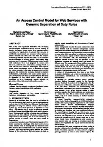
to know the best schedule to enjoy his three days in New York city. Assume there is a broadcast based wireless information system that covers the city of New York. Professor Edward has a wireless device that could be used to access the system. He hopes to use the information system to help schedule his stay. However, with the traditional wireless broadcast infrastructure, it is difficult for the professor to take full advantage of the system. First of all, since the system has no support for service discovery, the mobile device does not know what services to use to obtain required information. Also, the system does not facilitate collaboration of multiple services. Therefore, the professor would not be able to use the system to achieve complex requests such as scheduling tasks. In this research, we propose a new infrastructure to address these issues for traditional wireless broadcast systems. The proposed infrastructure applies the Web services technologies to wireless world. The registry and discovery technologies help mobile users find services of their interest. The service composition technologies can be used to define services that are dependent on other services. Similar to “wired” Web services, a basic wireless Web service (i.e. M-service) architecture would also consist of a service requester, a service provider and a discovery agency. M-services are made available to mobile users through wireless channels. Mobile users first look up specific M-services in a wireless service registry (discovery agency). The users then access the selected M-services through wireless channels by using the information obtained from the registry. Figure 2.1 shows a typical example of M-services systems. A service provider advertises its services by registering the description of these services with a wireless discovery agency. Similar to WSDL in Web services, the description contains information on how to access and invoke the services. The wireless discovery agency would make the service description available to mobile users on the wireless channels. These wireless channels are maintained by base transceiver stations. By accessing discovery agency’s wireless channels, mobile clients would find services that best meet users’ needs, and get information on how to access these services. The actual services are also made available through wireless channels. Mobile clients could


12

Figure 2.1: A Typical M-service System then retrieve the services and invoke their operations. Although Web services technologies are widely used, the challenge is how to support them in broadcast-based wireless environment. The proposed infrastructure covers the following aspects: • Broadcast content: The infrastructure defines what information needs to be available on broadcast channels to support broadcast-based M-services.

• Channel layout: The infrastructure defines different channel types and their organizations for delivering the defined broadcast content.

• Service/data retrieval: The infrastructure also defines how to retrieve services and wireless from broadcast channels.

2.2

Efficient Access to M-services and Wireless Data

Traditional wireless broadcast systems are normally data-centric. Mobile devices use pre-installed applications to access wireless data from broadcast channels. Stimu-


13

lated by the recent success in wireless technologies, the number of mobile users have been rapidly increasing over the past years. Wireless networks are capable of delivering much larger amount of data to mobile users. It is getting more and more difficult to support fast increasing wireless data and applications with the traditional datacentric infrastructure. As already discussed, no effective way is available for mobile users to discover or combine services. As a result, wireless paradigm is shifting from data-centric to service-centric. Modern wireless networks allow mobile users discover and access services of their interest. Our focus in this research is to design efficient access methods for retrieving services and wireless data in service-centric wireless broadcast systems. A lot of research work has been conducted in designing efficient data access methods for traditional wireless broadcast systems. These data access methods aim to help mobile users locate and access requested data in broadcast channels more efficiently. However, these methods are not suitable for the proposed infrastructure because accessing services is an inherently different process from accessing wireless data. Let us now look at how accessing information differs in data-centric and service-centric systems. Access pattern – Accessing data is usually considered as a “search and match” process. Mobile devices scan through broadcast channels based on their organizations and filtering criteria to locate requested items. Access methods for data centric systems only need to consider this “search and match” process. Accessing services, on the other hand, is a more complex process. It requires multiple steps. Users first need to discover suitable services. Then the selected services needs to be downloaded and executed. At last wireless data required by these services is retrieved. Access methods for service-centric systems need to take all these steps into consideration and try to make the whole process most efficient instead of just one single step. Service dependencies – There are two types of services, simple and composite. Composite services may need to invoke other services. Based on their BPEL definitions, these services could have certain dependencies between each other. This means services can only be executed conforming to the defined dependencies. Therefore, it is important to know the type of a service and its defined dependencies to


14

access and execute the service. Access methods for service-centric systems need to leverage the knowledge of these dependencies to achieve the best possible overall access efficiency. Service-data dependencies – When a service is executed, it might need to retrieve wireless data from broadcast channels. The retrieved data could be presented to users as part of final results or used by other services as intermediate results. The required wireless data will not be known until the service is executed. For composite services, access methods may need to dynamically adjust the access sequence based on the locations of the required wireless data to achieve better performance. For example, assume composite service S defines two parallel simple services S1 and S2. Based on the locations of these services, a mobile device is to access S2 right after S1. When S1 is executed, it asks for data D1. Based on the mobile device realizes that D1 will arrive before S2. The mobile device then adjusts the pre-defined access sequence and retrieves D1 before S2. Access semantics – Services and wireless data are delivered on a “push” instead of “pull” basis. This means some services might arrive when their dependencies are not fulfilled yet. On some mobile devices, based on available resources, they could be cached to be executed later. Alternatively, they would have to be downloaded on their next arrivals. It is important to understand these semantics and leverage such knowledge to achieve the best possible access efficiency. In this research, we define the semantics that have impact on access efficiency. Then we investigate efficient methods for accessing services taking these semantics into account.

2.3

Example Scenario

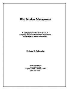
Let us use the same example presented in Section 2.1 to illustrate the use of broadcast based M-services. Assume the information system supports broadcast based Mservices. and there is a service called trip planner. The BPEL design of the service is shown in Figure 2.2, which is generated using Oracle JDeveloper BPEL Designer 10g. This service is a composite service that uses a few other services


15

to schedule trips for tourists based on their input. This service first invokes other required services to gather information and then calculates the best schedule.

Figure 2.2: Trip Planning Composite Service As shown in the BPEL graph, the trip planner service invokes six other services. First, it invokes attractions, entertainment, restaurants, and shopping services to let a user select activities for this trip. These services could be accessed and executed in parallel. Once the user makes the selections, the service would in-


16

voke transportation, traffic, and weather services to generate the best possible schedule. The schedule is generated based on the combination of serveral factors, such as the time and locations of activities, and weather conditions (e.g. outdoor activities are preferred on sunny days). The best transportation between any two consecutive activities would also take traffic conditions into consideration. This makes the traffic service to be dependent on the transportion service. The trip planner service could be re-executed anytime during the trip to update the existing schedule in the case of any unexpected events or change of the activities. This example scenario shows that one user request may result in retrieving multiple services. These services could be accessed and executed in different fashions (e.g. in sequence or parallel). Similarly, wireless data could also be retrieved in various ways by different services. Access methods for such an M-services system should support the variety of ways of efficiently accessing services and data based on different user requirements.

2.4

Overview of Main Contributions

In this section, we present the overview of our main contributions in this research. We first conduct an extensive study on a few existing access techniques for dataoriented wireless networks. Then we propose a few new data access methods that outperform the existing methods. We also develop a testbed for evaluating these data access methods. We conduct extensive experiments for comparing the existing and new access methods. We also study the behavior of accessing simple M-services using traditional access methods. Then we propose an infrastructure that supports both simple and composite services. We propose efficient access methods for the infrastructure and conduct extensive practical study on the proposed methods. Analytical and practical study on traditional data access methods – In recent years, several wireless data access methods have been proposed to improve data access efficiency in wireless environment. These methods are evaluated in different environment contexts defined by the authors. Hence, it is difficult for readers


17

to compare these methods because different environmental settings are used. To better analyze different access methods, we present a common analytical model for wireless environment. We define a set of commonly used environmental parameters that have impact on access efficiency. We also derive analytical cost models for a few most recognized access methods. Furthermore, a testbed has been developed to implement data access in wireless environment and simulate a wireless broadcast environment. The purpose of this testbed is to provide a platform to compare, evaluate, and help develop new access methods. The testbed supports several adjustable environmental settings for studying access methods under different settings. Extensive experiments have been conducted to compare the selected data access methods. New data access methods – An adaptive wireless data access method and some variations are proposed for wireless environment. The proposed method is based on the observation that the performances of existing methods are severely affected by environmental settings. This proposed method exhibits good overall performance and stabler performance when some important environmental settings change. By varying a construction factor, the proposed methods would yield different performance patterns. The testbed has been enhanced to support these new access methods. Simulation experiments have been conducted to compare the proposed methods to the existing ones. Efficient access to simple M-services using traditional techniques – We then extend our study on traditional access techniques to the M-services world. We study the behavior of accessing simple M-services using a few different traditional techniques. We assume mobile users are able to discover services of their interest using broadcast registry information. We derive analytical models for accessing simple M-services with traditional access techniques. The testbed is further enhanced to support accessing simple M-services. By using the testbed, we conduct practical study on accessing simple M-services using traditional access techniques. Broadcast-based M-services infrastructure – We propose a novel wireless broadcast infrastructure that supports discovery and composition of M-services. We define system roles for the infrastructure and present an interaction model which


18

defines how these system roles interact with each other. We also define the broadcast content for this infrastructure. The broadcast content contains all information mobile users need to discover, download, and execute simple and composite services. Semantic access to broadcast-based M-services – As already discussed, accessing M-services especially composite M-services is different from accessing static wireless data. In this research, we define semantics of accessing composite M-services and study how to leverage these semantics to achieve best possible access performance. We also propose a few channel organizations for efficiently accessing services and wireless data in the proposed infrastructure. We derive analytical models for the proposed channel organizations. Practical study on proposed access methods – A new testbed is developed to simulate the proposed M-services infrastructure. The testbed supports the defined access semantics for composite M-services. All proposed access methods and channel organizations are implemented in the testbed. We conduct extensive experiments to study the access efficiency of the proposed access methods and channel organizations. We also study the impact of different semantics on these methods.

Chapter 3 Traditional Data Access Methods Access efficiency has drawn a lot of research attention in the past few decades. Several wireless data access methods have been proposed to improve data access efficiency in wireless environment. These methods are evaluated in different environment contexts defined by the authors. Hence, it is difficult for readers to compare these methods because different environmental settings are used. To better analyze different access methods, we present a common analytical model for wireless environment. We define a set of commonly used environmental parameters that have impact on access efficiency. We selected a few most recognized access methods and derived analytical cost models for them. A testbed is developed to implement data access in wireless environment and simulate a wireless broadcast environment. The purpose of this testbed is to provide a platform to compare, evaluate, and help develop new access methods. The testbed supports several adjustable environmental settings for studying access methods under different settings. Extensive experiments have been conducted to compare the selected data access methods.

3.1

Basic Data Access Techniques

In recent years, several data access methods have been proposed to improve performance of data access by introducing indexing techniques to broadcast based wireless

Chapter 3. Traditional Data Access Methods

20

environments. Most of these methods are based on three basic techniques: index tree [24, 8, 50, 22, 48, 21, 55, 16], signature indexing [29, 9], and hashing [25]. Some methods are based on the combination of more than one of these techniques. For example, indexing methods taking advantages of both index tree and signature indexing techniques have been proposed in the past [54, 18, 19, 20]. In the rest of this section, we discuss these three basic techniques in details.

3.1.1

Index tree based access methods

B+ tree indexing is a widely used indexing technique in traditional disk-based environments. It is also one of the first indexing techniques applied to wireless environments. The use of B+ tree indexing in wireless environments is very similar to that of traditional disk based environments. Indices are organized in B+ tree structure to accelerate the search processes. An offset value is stored in each index node pointing at corresponding data item or lower level index node. However, there are some differences that introduce new challenges to wireless environments. For example, in disk based environments, offset value is the location of the data item on disk, whereas in wireless environments, offset value is the arrival time of the bucket containing the data item. A bucket is the basic logical unit of a broadcast channel, which usually contains a data item or several index entries with other access method specific information. Moreover, indices and data in wireless environments are organized in one-dimensional mode in broadcast channel. Missing the bucket containing index of the requested data item may cause the client to wait until the next broadcast cycle to find it again. The most representative B+ tree based methods are (1,m) indexing and distributed indexing [24]. We only discuss distributed indexing in this section, because it is derived from (1,m) indexing and they have very similar data structure.

21

Chapter 3. Traditional Data Access Methods 3.1.1.1

Data Organization

In distributed indexing, every broadcast data item is indexed on its primary key attribute. Indices are organized in B+ tree structure. Figure 3.1 shows a typical full index tree consisting of 81 data items [24]. Each index node has a number of pointers (in Figure 3.1, each node has three pointers) pointing at its child nodes. The pointers of the bottom level indices point at the actual data nodes. To find a specific data item, the search follows a top-down manner. The top level index node is searched first to determine which child node contains the data item. Then the same process will be performed on that node. This procedure continues till it finally reaches the data item at the bottom. The sequence of the index nodes traversed is called the index path of the data item. For example, the index path of data item 34 in Figure 3.1 is I, a2, b4, c12. I Replicated Part

a1

b1

a2

b2

b3

b4

b5

a3

b6

b7

b8

b9 Non-Replicated Part

c1

c2

c3

c4

c5

c6

c7

c8

c9

c10 c11 c12 c13 c14 c15 c16 c17 c18 c19 c20 c21 c22 c23 c24 c25 c26 c27

0

3

6

9 12 15 18 21 24 27 30 33 36 39 42 45 48 51 54 57 60 63 66 69 72 75 78

Figure 3.1: A sample index tree What was discussed so far is similar to the traditional disk-based B+ tree indexing technique. The difference arises when the index and data are put in the broadcast channel. A node in the index tree is represented by an index bucket in the broadcast channel. Similarly, a broadcast data item is represented by a data bucket. In the traditional disk-based systems, index and data are usually stored in different locations. The index tree is searched first to obtain the exact location of the

22


requested data item. This process often requires frequent shifts between index nodes or between index and data nodes. As data in a wireless channel is one-dimensional, this kind of shift is difficult to achieve. Therefore, in distributed indexing, data and index are interleaved in the broadcast channel. The broadcast data is partitioned into several data segments. The index tree precedes each data segment in the broadcast. Users traverse the index tree first to obtain the time offset of the requested data item. They then switch to doze mode until the data item arrives. Figure 3.2 illustrates how index and data are organized in the broadcast channel. In (1,m) indexing [24], the whole index tree precedes each data segment in the broadcast. Each index bucket is broadcast a number of times equal to the number of data segments. This increases the broadcast cycle and thus access time. Distributed indexing achieves better access time by broadcasting only part of the index tree preceding each data segment. The whole index tree is partitioned into two part: replicated part and non-replicated part. Every replicated index bucket is broadcast before the first occurrence of each of its child. Thus the number of times it is broadcast is equal to the number of children it has. Every non-replicated index node is broadcast exactly once, preceding the data segment containing the corresponding data records. Using the index tree in Figure 3.1 as an example, the first and second index segments will consist of index buckets containing nodes I, a1, b1, c1, c2, c3 and a1, b2, c4, c5, c6 respectively.

Broadcast Cycle Last broadcast key Offset to next broadcast Local indices Control indices Offset to next index segment

Index Segment

Index Bucket

Data Segment Data Offset to next index segment Data Bucket

Figure 3.2: Index and data organization of distributed indexing Each index bucket contains pointers that point to the buckets containing its child nodes. These pointers are referred to as local index. Since the broadcast is


23

continuous and users may tune in at any time, the first index segment users come across may not contain the index of the requested data item. In this case, more information is needed to direct users to other index segment containing the required information. Control index is introduced for this purpose. The control index consists of pointers that point at the next occurrence of the buckets containing the parent nodes in its index path. Again using the index tree in Figure 3.1 as an example, index node a2 contains local index pointing at b4, b5, b6 and control index pointing at the third occurrence of index node I. Assume there is a user requesting data item 62 but first tuning in right before the second occurrence of index node a2. The control index in a2 will direct the user to the next occurrence of I, because data item 62 is not within the subtree rooted at a2. 3.1.1.2

Access Protocol

The following is the access protocol of distributed indexing for a data item with key K: mobile client requires data item with key K tune into the broadcast channel keep listening until the first complete bucket arrives read the first complete bucket go to the next index segment according to the offset value in the first bucket (1) read the index bucket if K < Key most recently broadcast go to next broadcast else if K = Key being broadcast read the time offset to the actual data records go into doze mode tune in again when the requested data bucket comes download the data bucket


24

else read control index and local index in current index bucket go to higher level index bucket if needed according to the control index go to lower level index bucket according to the local index go into doze mode between any two successive index probes repeat from (1)

3.1.2

Signature indexing

A signature is essentially an abstraction of the information stored in a record. It is generated by a specific signature function. By examining a record’s signature, one can tell if the record possibly has the matching information. Since the size of a signature is much smaller than that of the data record itself, it is considerably more power efficient to examine signatures first instead of simply searching through all data records. Access methods making use of signatures of data records are called signature indexing. Three signature indexing based access methods, simple signature, integrated signature, and multi-level signature, are proposed in [29]. The integrated and multi-level signature indexing methods are based on the simple signature indexing method and designed to handle more complex data structures. We only discuss the simple signature method in this section. The signatures are generated based on all attributes of data records. A signature is formed by hashing each field of a record into a random bit string and then superimposing together all the bit strings into a record signature. The number of collisions depends on how perfect the hashing function is and how many attributes a record has. Collisions in signature indexing occur when two or more data records have the same signature. Usually the more attributes each record has, the more likely collisions will occur. Such collisions would translate into false drops. False drops are situations where clients download the wrong data records which happen to have matching signatures.

25

Chapter 3. Traditional Data Access Methods 3.1.2.1

Data Organization

In signature based access methods, signatures are broadcast together with data records. The broadcast channel consists of index (signature) buckets and data buckets. Each broadcast of a data bucket is preceded by a broadcast of the signature bucket, which contains the signature of the data record. For consistency, signature buckets have equal length. Mobile clients must sift through each broadcast bucket until the required information is found. The data organization of simple signature indexing is illustrated in Figure 3.3.

Broadcast Cycle

Signature

Data Record

Figure 3.3: Data organization of signature indexing

3.1.2.2

Access Protocol

The access protocol for simple signature indexing is as follows (assume K and S are the key and signature of the required record respectively, and K(i) and S(i) are the key and signature of the i-th record): mobile client requires data item with key K tune in to broadcast channel keep listening until the first complete signature bucket arrives (1) read the current signature bucket if S(i) = S(k) download the data bucket that follows it if K(i) = K search terminated successfully


26

else false drop occurs continue to read the next signature bucket repeat from (1) else go to doze mode tune in again when the next signature bucket comes repeat from (1)

3.1.3

Hashing

Hashing is another well-known data access technique for traditional database systems. In this subsection, we introduce a simple hashing method, which was proposed for broadcast based wireless environments [25]. 3.1.3.1

Data Organization

Simple hashing method stores hashing parameters in data buckets without requiring separate index buckets or segments. Each data bucket consists of two parts: Control part and Data part. The Data part contains actual data record and the Control part is used to guide clients to the right data bucket. The data organization of the broadcast channel using simple hashing is illustrated in Figure 3.4.

Bucket

Broadcast Cycle

Shift: pointer to the actual bucket Hash Function: h Control Part

Data Part

Figure 3.4: Index and data organization of simple hashing The control part of each data bucket consists of a hashing function and a shift value. The hashing function maps the key value of the data in the broadcast data


27

record into a hashing value. Each bucket has a hashing value H assigned to it. In the event of a collision, the colliding record is inserted right after the bucket which has the same hashing value. This will cause the rest of records to shift, resulting in data records being ”out-of-place”. The shift value in each bucket is used to find the right position of the corresponding data record. It points to the first bucket containing the data record with the right hashing value. Assume the initial allocated number of buckets is Na . Because of collisions, the resulting length of the broadcast cycle after inserting all the data records will be greater than Na . The control part of each of the first Na buckets contains a shift value (offset to the bucket containing the actual data record with the right hashing value), and the control part of each of the remaining data buckets contains an offset to the beginning of the next broadcast. 3.1.3.2

Access Protocol

Assume the hashing function is H, thus the hashing value of key K will be H(K). The access protocol of hashing for a data item with key K is: mobile client requires data item with key K tune into the broadcast channel keep listening until the first complete bucket arrives (1) read the bucket and get the hashing value h if h < H(K) go to doze mode tune in again when h = H(K) (hashing position) else go to doze mode tune in again at the beginning of the next broadcast repeat from (1) read shift value at the bucket where h = H(K) go to doze mode tune in again when the bucket designated by the shift


28

value arrives (shift position) keep listening to the subsequent buckets, till the wanted record is found search terminated successfully or a bucket with different hashing value arrives search failed

3.2

Analytical Study

Access Time and Tuning Time are the two factors that are commonly used to measure the efficiency of wireless data access methods. The access time refers to the total time mobile clients need to wait for the request to complete. The tuning time is the actual time spent by mobile clients to actively listen to wireless channels and process requests. Request processing requires CPUs to stay busy. Listening to wireless channels means that receiving devices are actively retrieving data from wireless channels. Since most power consuming parts of a mobile unit are CPU and receiving devices [66], the tuning time of a request is usually proportional to the power consumed by a mobile unit on the request. Data Access Methods are used to improve the efficiency (usually the power consumption) of wireless data access. Several data access methods have been proposed in recent years to conserve power consumption in wireless environments. Each of them has its own advantages and drawbacks. However, since these methods are presented with different environmental settings, it is difficult to compare them in quantitized manner. In this section, we first define a basic wireless environment that provides mobile users with information through wireless broadcast channels. The environment will be served as unified context to evaluate various access methods. Then we present the analytical evaluation models for the selected access methods under the unified environment.


3.2.1

29

Basic Broadcast-based Wireless Environment

In the basic broadcast-based wireless environment, we assume there is only one broadcast channel because most of the existing wireless data access methods are proposed for single channel scenario. A mobile user obtains the required information by listening to the broadcast channel till the data of interest is broadcast and downloaded to the mobile client. We define the following parameters for the environment: System parameters Nr

Number of broadcast data items

N

Number of total buckets

Sdk

Key size of data items

Sd

Data item size

Sb

Logical broadcast unit (bucket) size

Bc

Broadcast cycle - the length of all contents in the broadcast channel

Bd

Broadcast channel bandwidth

Performance measurement parameters At

Access time

Tt

Tuning time

Bt

Broadcast cycle time - time to scan the whole broadcast channel

It

Time to browse an index bucket

Dt

Time to browse a data bucket

Ft

Time to reach the first complete bucket (initial wait) Table 3.1: Symbols and parameters for data access methods

Since the time that a user start listening is totally random, the mobile client may hit in the middle of a broadcast bucket after tuning into the broadcast channel. The initial wait time is the time spent to reach the first complete bucket after tuning into the broadcast channel. The number of broadcast data items (Nr ), represents


30

the number of data items being broadcast in a broadcast cycle. The number of total buckets (N ) designates the total number of buckets in a broadcast cycle, including data buckets (containing data items), index buckets (containing indices in index tree based methods), and hashing buckets (containing hash values in hashing based methods). When there is no access method (flat broadcast), users must keep listening to the broadcast channel until the required data item arrives. Therefore, the average access time and tuning time are half of the whole broadcast cycle plus the initial wait time, which can be expressed as follows:

At = Tt = Ft + Bt 1 = ( + N r ) × Dt 2

3.2.2

Cost model for index tree based access methods

We now derive the access and tuning times for index tree based access methods. First, we define symbols which are specific to these methods. Let n be the number of indices contained in an index bucket, let k be the number of levels of the index tree, and let r be the number of replicated levels. It is obvious that k = ⌈logn (Nr )⌉.

The access time consists of three parts: initial wait, initial index probe, and broadcast wait. initial wait (Ft ): It is the time spent to reach the first complete bucket. Obviously we have:

Dt 2 initial index probe (Pt ): This part is the time to reach the first index segment. Ft =

It can be expressed as the average time to reach the next index segment, which is calculated as the sum of the average length of index segments and data segments.

31


Given the number of replicated level is r, the number of replicated index (Nrp ) is: 1 + n + ... + nr−1 =

nr − 1 n−1

The number of non-replicated index (Nnr ) is: nr + nr+1 + ...nk−1 =

nk − nr n−1

As we mentioned before, each replicated index is broadcast n times and each nonreplicated index is broadcast exactly once. Thus the total number of index buckets can be calculated as: Nrp × n + Nnr = n ×

nk + nr+1 − nr − n nr − 1 nk − nr + = n−1 n−1 n−1

The number of data segments is nr because the replicated level is r. Thus the average number of index buckets in an index segment is: 1 nr − 1 nk − nr nk−r − 1 nr+1 − n × (n × + ) = + nr n−1 n−1 n−1 nr+1 − nr The average number of data buckets in a data segment is

Nr . nr

Therefore, the initial

index probe is calculated as: 1 nk−r − 1 nr+1 − n Nr Pt = × ( + r+1 + r ) × Dt r 2 n−1 n −n n broadcast wait (Wt ): This is the time from reaching the first indexing segment to finding the requested data item. It is approximately half of the whole broadcast cycle, which is

N 2

× Dt . Thus, the total access time is: At = Ft + Pt + Wt

1 nk−r − 1 nr+1 − n Nr = ×( + r+1 + + N + 1) × Dt 2 n−1 n − nr nr The tuning time is much easier to calculate than access time, because during most of the probes clients are in doze mode. The tuning time includes the initial wait ( D2t ), reading the first bucket to find the first index segment (Dt ), reading the control


32

index to find the segment containing the index information of the requested data item (Dt ), traversing the index tree (k × Dt ), and downloading the data item (Dt ).

Thus, the tuning time is:

3.2.3

1 Tt = (k + 3 ) × Dt 2

Cost model for signature indexing

For signature indexing, clients must scan buckets one by one to find the required information, the access time is determined by the broadcast cycle. A signature bucket contains only the signature of a data record. No extra offset or pointer value is inserted into the signature/index bucket as in other access methods. Since the total length of all data records is a constant, the length of signatures is the only factor that determines the broadcast cycle. Access time, therefore, is determined by the length of signature buckets. The smaller the signatures are, the better the access time is. As for tuning time, it is determined by two factors: the size of signature buckets and the number of false drops. It is obvious that smaller signature lengths reduce tuning time. However, smaller signature sizes usually implies more collisions or false drops. In cases of false drops, wrong data records are downloaded by mobile clients, resulting in longer tuning time. From this analysis, we observe two tradeoffs: (1) signature length against tuning time, and (2) access time against tuning time. Signature indexing uses two types of buckets (with varying sizes): signature bucket and data bucket. The initial wait is the time to reach the closest signature bucket:

1 × (Dt + It ) 2 As discussed above, the access time is determined by the broadcast cycle. It consists Ft =

of two parts: the initial wait (Ft ) and the time to browse the signature and data buckets (SDt ). The average value of SDt for retrieving a requested bucket is half of the broadcast cycle ( 21 × (Dt + It ) × Nr ). Therefore, the access time is: At = Ft + SDt

33

Chapter 3. Traditional Data Access Methods 1 1 × (Dt + It ) + × (Dt + It ) × Nr 2 2 1 = × (Dt + It ) × (Nr + 1) 2 =

The tuning time is determined by both the length of index buckets and the number of false drops. It consists of three parts: the initial wait (Ft ), the time to browse signature buckets (SBt ), and the time to retrieve false drop data buckets (F Dt ) and the requested data bucket (Dt ). The average value of SBt is half of the total length of signature buckets, which is

1 2

× It × Nr . Assuming Fd is the number

of false drops, the value of F Dt will be Fd × Dt . Hence the resulting tuning time is:

Tt = Ft + SBt + F Dt + Dt 1 1 = × (Dt + It ) + × It × Nr + Fd × Dt + Dt 2 2 1 1 = × (Nr + 1) × It + (Fd + 1 ) × Dt 2 2

3.2.4

Cost model for hashing

The access time of the hashing method consists of an initial wait time (Ft ), time to reach the hashing position (Ht ), time to reach the shift position (St ), time to retrieve colliding buckets (Ct ), and time to download the required bucket (Dt ). Since there is only one type of bucket used in hashing, the initial wait is Ft =

Dt . 2

Let Nc be

the number of colliding buckets, the average number of shifts of each bucket is thus Nc . 2

Therefore, we have St =

Nc 2

× Dt . Furthermore, the average number of colliding

buckets for each hashing value is

Nc . Nr

Thus, we have Ct =

Nc Nr

× Dt . The calculation

of Ht is more involved. Assume the number of initially allocated buckets is Na . The resulting total number of buckets in the broadcast cycle is N = Na + Nc . We have the following three possibilities that result in different values of Ht (assume the position of the first arriving bucket is n). Ht1 =

Nc 1 × ( × (Nc + Na )) N 2

(n > Na )

34


1 Na Na × × (n ≤ Na and request item broadcast = F alse) 2 N 3 Na Na 1 Na ×( + Nc + ) (n ≤ Na and request item broadcast = T rue) Ht3 = × 2 N 3 3

Ht2 =

The request item broadcast above designates if the requested information has already been broadcast in the current broadcast cycle.

The first part of each

formula above is the probability the scenario will happen. As a result, we have Ht = Ht1 + Ht2 + Ht3 . Based on the above discussion, the access time is:

At = Ft + Ht + St + Ct + Dt = Ft + Ht1 + Ht2 + Ht3 + St + Ct + Dt 1 N 1 =( + + N − × N a ) × Dt 2 Na 2 The tuning time consists of an initial wait time (Ft ), time to read the first bucket to obtain the hashing position (Dt ), time to obtain the shift position (Dt ), and time to retrieve the colliding buckets (Ct ), and time to download the required bucket (Dt ). The probability of collision is

Nc . Nr

Thus, we have Ct =

Nc Nr

× Dt . For those requests

that tune in at the time which the requested bucket has already been broadcast, one extra bucket read is needed to start from the beginning of the next broadcast cycle. The probability of this scenario occurrence is (Nc + 21 × Nr )/(Nc + Nr ). As a result, the expected tuning time is:

1 Nc + 12 × Nr Nc Tt = ( + + + 3) × Dt 2 Nc + Nr Nr

3.3

Testbed

This section presents the testbed we developed for the evaluation of data access methods in wireless environments. The testbed is implemented in Java language

35


using the JavaSim simulation package [43] [31]. The testbed simulates data access for traditional wireless environments. The testbed is event-driven. The broadcasting of each data item, generation of each user request and processing of the request are all considered to be separate events in this testbed. They are handled independently without interference with each other. We call the testbed adaptive because (1) it can be easily extended to implement new data access methods; (2) it is capable of simulating different application environments; (3) new evaluation criteria can be added. The components of the testbed are described as follows:

RequestGenerator

ResultHandler

uses

AccuracyController

creates

Simulator Request

Request creates

listens to

... Bucket Bucket

initializes

...

Request

listens to

...

listens to

Bucket Bucket Bucket

...

BroadcastChannel Data Source

uses

BroadcastServer

constructs

Channel

Figure 3.5: Testbed Architecture

Simulator: The Simulator object acts as the coordinator of the whole simulation process. It reads and processes user input, initializes data source, and starts broadcasting and request generation processes. It also determines which data access method to use according to the user input. BroadcastServer: It is a process to broadcast data continuously. The BroadcastServer constructs broadcast channel at the initialization stage according to the input parameters and then starts the broadcast procedure.


36

RequestGenerator: RequestGenerator is another process initialized and started by the Simulator. It generates requests periodically based on certain distribution. In the simulations covered by this proposal, the request generation process follows exponential distribution. Data: Information to be broadcast is represented by a Data object. The information is read from files or databases. The Data object consists of a number of records. Record: It is used to represent a broadcast data item. Each record has a primary key and a few attributes. Bucket: Broadcast data items are reorganized as buckets to put in broadcast channel. A bucket can be either index (signature) or data. The Bucket object is used to represent such bucket. Different access methods have different bucket organization. Channel: The Channel object consists of a number of Buckets. It is constructed at initialization stage based on which data access method is being used. The BroadcastServer process broadcasts information contained in the broadcast Channel. Request: User request is represented by Request objects. Each request is considered to be an independent process. Once generated by the RequestGenerator, it starts listening to the broadcast channel for the required data item till it is found. ResultHandler: In our testbed, we use access time and tuning time as criteria to evaluate the performance of the access methods. The ResultHandler object extracts and processes the simulation results and output them in the proper format. AccuracyController: To ensure the accuracy of our simulation, we use an AccuracyController object to control the accuracy of the simulation results. Users

37


can specify the accuracy expectation for the simulation. The simulation process will not terminate unless the expected accuracy is achieved. We also implemented the analytical evaluation model of each access method in the testbed so that we can compare the simulation results against the theoretical results. The testbed supports the following environmental parameters that may have influence on the performance of access methods: Nr

Number of broadcast data items

Sdk


Sd

Data item size

Bd

Broadcast channel bandwidth

Da

Data availability

Cl

Confidence level

Ca

Confidence accuracy

Dr

Distribution for request interval

Table 3.2: Supported testbed parameters The data availability defines the possibility of the requested information to be present in broadcast channel. In real settings, the requested information may not exist at all in the broadcast channel. How data availability affects performance becomes an important issue and worthwhile investigating. In applications with very low data availability, access methods requiring one-at-a-time browsing have usually very poor efficiency because clients scan the whole broadcast channel. Whereas for some other access method, such as distributed indexing, the performance is better with very low data availability because clients only need to scan the indexing section to determine the presence of requested information. The confidence level and confidence accuracy

1

are used to control the accuracy

of the simulation results. Users can specify the values of confidence level and accuracy before starting simulation. The simulation is not complete until the expected


38

confidence level and accuracy are achieved. The request interval parameter determines which distribution (e.g. exponential distribution) the testbed follows to generate requests. This parameter can be used to simulate different access patterns. Figure 3.5 shows the generic architecture of the testbed. When a particular data access method is used, specific objects are created. For example, if user chooses to use signature indexing, the BroadcastServer constructs a SigChannel which would consist of a number of SigBuckets. The RequestGenerator would periodically generate SigRequests. The Simulator would create a SigResultHandler object to process the signature indexing specific results. The generic objects only store information that is common to all data access methods. The testbed is implemented as a discrete event driven simulation system. The following procedures explain how the testbed works: • Initialization stage: – Create Simulator object – Simulator initializes the Data object, BroadcastServer object, RequestGenerator object and specific ResultHandler object. – Data object reads the data source and creates all Record objects. – Depending on which access method is selected, BroadcastServer creates the corresponding Channel object. – Specific Channel object is created. A number of corresponding Bucket objects are created based on data records. Buckets are inserted into the 1

Given N sample results Y1 , Y2 , ..., YN , the confidence accuracy is defined as H/Y, where H is the

confidence interval half-width and Y is the sample mean of the results (Y = (Y1 + Y2 + ... + YN )/N ). The confidence level is defined as the probability that the absolute value of the difference between the Y and µ (the true mean of the sample results) is equal to or less than H. H is defined by √ H = tα/2;N −1 × σ/ N where σ 2 is the sample variance given by σ 2 = Σi (Yi − Y )2 /(N − 1) (thus σ is the standard deviation), and t is the standard t distribution.


39

broadcast channel according to the data organization of the chosen data access method. • Start stage: – Simulator starts BroadcastServer. – Simulator starts RequestGenerator. • Simulation stage: – Broadcast channel broadcasts the information continuously. – RequestGenerator generates Request periodically using the exponential distribution. – Generated requests listen to the broadcast channel and query the required information. – When completed, Request objects inform ResultHandler object of the results. – Simulator checks if the results are within the expected confidence and accuracy level to determine whether to terminate or continue the simulation. • End stage: – Simulator stops BroadcastServer. – Simulator stops RequestGenerator. – ResultHandler processes the results and outputs them in a proper format. A integrated GUI is developed for easy usage. Figure 3.6 shows a running example of the testbed GUI. The graphical user interface (GUI) allows users to input parameters, execute the logic, and view the results. It also allows users the ability to display graphical plots


40

Figure 3.6: Testbed Client GUI (e.g. Cartesian graphs). The GUI has user controls for data storage, such as, save test results (input and output values), retrieve test results from previous test, and delete test results.


3.4

41

Practical Study

We now present some experiment results for a few existing wireless data access methods. We show both practical and theoretical results for each method. The practical results are obtained by running experiments using each access method, and the theoretical results are produced from the formulas presented in Section 3.2. By comparing practical results against theoretical results, we show the correctness of our system implementation and the predictiveness of the analytical cost model. As a benchmark, we also show the experiment results for broadcasting without using any data access method, i.e., flat or plain broadcast.

3.4.1

Simulation Settings

The data source our testbed uses is a dictionary database consisting of about 35,000 records. Table 3.3 shows the simulation settings for all experiments presented in this section: Data type

text

Number of records

7000 - 34000

Record size

500 bytes

Key size

25 bytes

Number of requests

> 50000

Confidence level

0.99

Confidence accuracy

0.01

Request interval

exponential distribution

Table 3.3: Simulation settings for data access methods The testbed reads the data records from the data source and constructs them into data buckets using specific access methods. The access time and tuning time of each access method are evaluated in terms of the number of bytes read. Often


42

possible parameters like the number of buckets or actual time elapsed are not used for the following reasons: 1. Bucket sizes may vary depending on the access method. 2. Some access methods use varied bucket sizes. For example, signature indexing uses two types of buckets, data bucket and signature bucket. Their sizes are different. 3. There are many factors that may affect time measurement during simulation, such as CPU speed, network delay, CPU workload, etc. Mobile user requests are simulated through a random request generator. During each simulation round, there are 500 requests generated. At the end of the round, the result is checked against the confidence level and confidence accuracy. The simulation continues if the confidence conditions are not satisfied. In most of our simulation experiments, more than 100 simulation rounds are required to satisfy the confidence conditions we defined in Table 3.3. The generation of requests follows the exponential distribution. In all simulation experiments discussed in this section, we assume all requested data records are found in the broadcast.

3.4.2

Simulation Results

Based on the above simulation settings, each access method is simulated using the testbed. Figure 3.7 shows the simulation results for flat broadcast, distributed indexing, signature indexing and simple hashing. The lines marked with (S) are simulation results. Those marked with (A) are analytical results. We observe in both figures that the simulation results match the analytical results very well. Flat broadcast exhibits the best access time but worst tuning time. With the introduction of data access methods, extra information is inserted into broadcast channel to help clients get to the required data item. This also introduces overhead in the broadcast cycle that consequently increases access time. In the flat broadcast,

43

Chapter 3. Traditional Data Access Methods (a) Access Time vs. Number of Data Records

(b) Tuning Time vs. Number of Data Records

1.6e+07

10000 distributed indexing (S) distributed indexing (A) simple hashing (S) simple hashing (A) flat broadcast (S) flat broadcast (A) signature indexing (S) signature indexing (A)

Access Time (At)

1.2e+07 1e+07

distributed indexing (S) distributed indexing (A) simple hashing (S) simple hashing (A) signature indexing (S) signature indexing (A)

8000 Tuning Time (Tt)

1.4e+07

8e+06 6e+06

6000

4000

4e+06 2000 2e+06 0

0 0

5000

10000 15000 20000 25000 No. of Data Records

30000

35000

0

5000

10000

15000 20000 25000 No. of Data Records

30000

35000

Figure 3.7: Comparison for different access methods information is broadcast over the wireless communication channel without using any access method. Mobile clients must traverse all buckets to find the requested data. In such a case, mobile clients keep listening to the broadcast channel. This results in the worst tuning time. The expected average access time and tuning time are the same, which is approximately half of the broadcast cycle. Both access time and tuning time increase linearly with number of broadcast data records. From the formula presented in Section 3.2.2, since Dt is a constant, it is obvious that the tuning time of distributed indexing is determined by k, the number of levels in the index tree. The increase in the number of broadcast data records does not necessarily increase the tuning time, unless the bottom level of the index tree is filled and the number of levels in the index tree is, as a result, increased. The simulation result shows the same trend. We can also observe that the tuning time of distributed indexing only increases at one point (somewhere between 5000 and 10000 data records), where the number of levels in index tree is increased. The value of tuning time is much less than that of flat broadcast. With the help of indices, clients selectively listen to the broadcast channel, thus reducing the tuning time drastically. From Figure 3.7(a), we see that simple hashing has the worst performance in terms of access time. This is because simple hashing introduces more overheads to


44

the broadcast cycle. However, simple hashing has the best tuning time, as shown in Figure 3.7(b). According to the analysis in Section 3.1.3, it takes no more than four probes to reach the first bucket containing the requested hashing value. The tuning time is only determined by the average number of buckets containing the requested hashing value, which is the average overflow. Since we use the same hashing function for varied number of broadcast data records, the overflow rate is a fixed value. That is why we observe a straight horizontal line in the figure. Depending on how good the hashing function is, simple hashing achieves different average tuning times. Generally, it outperforms most of other access methods in terms of tuning time. As shown in Figure 3.7(a), signature indexing achieves a much better access time than all other access methods. The only overhead signature indexing introduces in broadcast cycle is the signatures of data records. Signatures are usually very small in size compared to the size of data records. Furthermore, unlike other access methods, there is no extra offset pointers in broadcast buckets (signature buckets or data buckets). The resulting broadcast cycle of signature indexing is smaller than that of other access methods, translating in smaller access time. Similar to the flat broadcast, signature indexing requires clients to serially browse through the broadcast buckets. The only difference is that signature is read first each time. Clients do not read the successive data buckets unless the signature matches the signature of the requested data record. Therefore, the tuning time of signature indexing is much larger than that of other access methods. We also note that the tuning time increases linearly with the number of broadcast data records. This is because when the signature length is fixed, increasing the number of broadcast data records leads to a larger number of signature buckets and false drops, which in turn result in a larger tuning time.


3.4.3

45

Comparison

In this section, we compare the access methods under different scenarios. We define the following two parameters: (1) Data availability which defines the possibility of the requested information to be present in broadcast channel, and Record/key ratio which is the proportion of record size to key size. In real settings, the requested information may not exist at all in the broadcast channel. How data availability affects performance becomes an important issue. In applications with very low data availability, access methods requiring one-at-a-time browsing have usually very poor efficiency because clients scan the whole broadcast channel. In other access methods, such as distributed indexing, however, clients only need to scan the indexing section to determine the presence of requested information. The record/key ratio is another important factor that may affect the efficiency of different access methods. For B+ tree based access methods, such as distributed indexing, higher record/key ratio implies more indices likely to be placed in a single bucket, which in turn would reduce the number of index tree levels. As previously discussed, tuning time is mainly determined by the number of index tree levels in these two access methods. Therefore, record/key ratio has a substantial influence on the performance of B+ tree based access methods. Record/key ratio has also great impact on the efficiency of signature or hashing based access methods. Smaller record/key ratio usually means less overhead being introduced to the broadcast cycle, which results in better access time. However, smaller record/key ratio may also lead to more false drops in signature indexing and higher overflow in hashing, causing worse tuning time. In real world applications, record/key ratios in different wireless applications may vary largely. Therefore, it is important to study how record/key ratio affects the efficiency of access methods. 3.4.3.1

Comparing access methods Based on Data Availability

We vary data availability from 0% to 100% in our simulation to evaluate the performance of different access methods. Figure 3.8 shows the result of access time and

46

Chapter 3. Traditional Data Access Methods tuning time against data availability. (a) Access Time vs. Data Availability

(b) Tuning Time vs. Data Availability

3e+06

22000 signature (1,m) distributed hashing

20000 2.5e+06


Access Time (At)

16000 2e+06 1.5e+06 1e+06

12000 10000 8000 6000

plain broadcast signature (1,m) distributed hashing

500000

14000

4000 2000

0

0 0

20

40

60

Data Availability (%)

80

100

0

20

40

60

80

100

Data Availability (%)

Figure 3.8: Comparison for different data availability Figure 3.8(a) clearly shows that data availability in hashing has little impact on access time. This is because changing the data availability does not change broadcast cycle and the access sequence of hashing method is only determined by the hashing function. We note that when the data availability is high (towards 100%), flat broadcast and signature indexing have the best performance. When the data availability is low (towards 0%), (1,m) indexing and distributed indexing outperform all other methods. The reason is that (1,m) indexing and distributed indexing can determine the presence of the requested information by reading only the index segment. As to tuning time, we do not consider it for flat broadcast simply because it is much larger than that of all other methods. Tuning time of signature indexing decreases with the increased data availability. This is because when data availability increases, there is less probability that clients scan the whole broadcast cycle to find out whether the requested record is in the broadcast. Figure 3.8(b) shows that (1,m) and distributed indexing perform better under low data availability, whereas signature indexing and hashing have better performance when data availability is high. For (1,m) and distributed indexing, it only takes a few probes (by reading only a few levels of index tree) to determine whether the requested information is


47

present. Therefore, they have the best performance when there is very low data availability. However, when data availability is high, extra probes are needed to find the actual data buckets in the broadcast. Therefore, the tuning time increases with data availability. For the hashing method, all overflow buckets must still be read when the requested information is not in the broadcast. It outperforms (1,m) indexing and distributed indexing at high data availability because it may need to read fewer overflow buckets before reaching the required bucket. 3.4.3.2

Comparing access methods Based on Record/Key Ratio

In this experiment, we assume that data availability is achieved at 100%. We vary the record to index ratio from 5 to 100. This is a reasonable range that record/key ratios of data in most applications fall in. The simulation results are shown in Figure 3.9. Figure 3.9(a) shows that access time changes with the record to key ratio. We see that the ratio has a strong impact only on (1,m) indexing and distributed indexing. That is because different record to key ratios may result in different index tree structures. For B+ tree based access methods, the ratio changes the number of buckets in the index tree and thus the index levels. For distributed indexing, the ratio also changes the number of replication levels. Figure 3.9(a) shows that both (1,m) indexing and distributed indexing have very large access times when the record to key ratio is small. This is because the overhead introduced by adding the index segment, is prominent when the key size is comparable with the record size. They perform much better when the ratio is large. Both (1,m) indexing and distributed indexing outperform hashing as record/key ratio gets larger. As to tuning time, flat broadcast is ignored because it is not comparable with the other methods. From our previous discussion, the tuning time of hashing is much better than that of other access methods. Figure 3.9(b) shows that (1,m) indexing and distributed indexing exhibit similar performance to hashing when the record/key ratio is large. The explanation is similar to that of access time. When

48

Chapter 3. Traditional Data Access Methods (a) Access Time vs. Record/Key Ratio

(b) Tuning Time vs. Record/Key Ratio

4e+06

12000 plain broadcast signature (1,m) distributed hashing


Access Time (At)

3.5e+06 3e+06 2.5e+06 2e+06

signature (1,m) distributed hashing

8000

6000

4000

1.5e+06 1e+06

2000 0

10

20

30

40 50 60 Record/Key Ratio

70

80

90

100

0

10

20

30

40 50 60 Record/Key Ratio

70

80

90

100

Figure 3.9: Comparison for different record/key ratio the key size is large compared to the data record, fewer indices fit into a single bucket. Thus, more buckets are read to traverse the index tree. This results in a larger tuning time. On the other hand, smaller key sizes result in smaller tuning time for (1,m) indexing and distributed indexing.

3.5

Summary

Based on the simulation and comparison presented above, we note the following observations: (1) Flat broadcast has the best access time but the worst tuning time. Since the tuning time of flat broadcast is far larger than that of any access methods, it is usually not a preferred method in power limited wireless environments; (2) Signature indexing achieves better access time than most of the other access methods. However, the tuning time of signature indexing is comparatively larger. When energy is of less concern than waiting time, signature indexing is a preferred method; (3) Hashing usually achieves better tuning time. In energy critical applications, hashing method (with a good hashing function) is preferred; (4) (1,m) indexing and distributed indexing achieve good tuning time and access time under low data availability. Therefore, they are a better choice in applications that exhibit frequent search failures; (5) (1,m) indexing and distributed indexing have


49

good overall performance (both access time and tuning time) when the key size of the broadcast data is very small compared to the record size. If access time is of concern, (1,m) indexing is preferable, otherwise distributed indexing is preferable.

Chapter 4 Adaptive Data Access Methods In this chapter, we present an adaptive method we proposed to improve efficiency of wireless data access. The proposed method is based on the observation that the index tree based methods preserve good access time as well as stable overall performance and that the hashing method exhibits good tuning time. By combining these two techniques, the new method takes the advantages of both techniques. As a result, it exhibits greater flexibility and better performance. As previously shown, the tuning time of hashing depends on Nc , which in turn depends on the number of collisions. The number of collisions normally depends on how good the hashing function is. Thus, deriving a good hashing function is crucial for good tuning time. However, because of the heterogeneity of broadcast data in different applications, this is usually difficult to achieve. Furthermore, the hashing function itself is included in every data bucket. This obviously increases the broadcast cycle, and thus, the access time. In our method, hashing is used only to partition the broadcast data into a number of partitions. B+ tree technique is then used to index each partition. The hashing function is only stored at the beginning of each partition. Since the number of partitions is a small number compared to the number of all data items, the overhead introduced is much smaller than that in hashing based method. We now show how hashing and index tree techniques are combined in our method:

Chapter 4. Adaptive Data Access Methods

51

• First level hashing: Generate hashing value (h1 ) for key attribute of each data item using a hashing function H1 . The hashing value generated at this step is

similar to the hash value in simple hashing method. • Second level hashing: Use another hashing function (H2 ) to produce p second

level hashing values (h2 ) based on the value of h1 generated in the first step.

This process will partition the broadcast data into p parts. All data items having the same second level hashing value will be in the same partition. • Generating the index tree: Within each partition, generate an index tree on the key attributes of the data items in the partition.

The two level hashing can actually be combined into one hashing method. We split it into two levels to better illustrate the steps. The adaptive method has the following advantages compared with simple hashing and distributed indexing: • Hashing is used only to partition the broadcast data. The number of partitions is a small number compared to the size of data items. Thus, it is much easier to

find hashing functions that generate hash codes with low conflicts on partitions than on all data items. • Hashing functions need only be included in front of each data partition. This reduces the broadcast cycle and as a result, the access time.

• The index tree levels of data items in one partition is smaller than that of all data items (the exact number is determined by p). This may result in

an improvement in tuning time because the tuning time is determined by the levels of index tree in each partition plus the overhead introduced by reading the hashing functions.

52


4.1

Data Organization

In the adaptive method, a data partition together with its associated index tree form a broadcast partition. At the beginning of each broadcast partition, hashing functions and the hashing value of this partition are stored. This information is used to locate the partition that contains the requested data item. Figure 4.1 illustrates how the broadcast channel is organized for the adaptive method. Broadcast Segment

Broadcast Cycle

Index Tree Indices

Hashing value Hashing function 1 Hashing function 2

Next partition

Data

Data Buckets

Next partition

Index Bucket

Figure 4.1: Channel structure of adaptive method

Hashing is used to locate the partition that the requested data item belongs to. The index tree helps to find the data item in the partition. Users only need to check the hashing value at the beginning of each partition to determine if the requested data item is in the coming partition. A match implies the requested data item is in this partition. If the hashing values do not match, the request will be forwarded to the right partition. The index tree of each partition is placed right after the hashing bucket(s) in the broadcast channel. This is different from distributed indexing where the index tree is partitioned. Instead, the whole tree (only for the data items in this partition) is used because there is no sub-partitions. Data buckets are placed following the index tree in each partition. Each bucket, index or data, has a pointer entry pointing to the next nearest partition. To divide the broadcast cycle into p partitions using hashing, we first use one or more hashing functions to generate hashing values H (1 ≤ H ≤ p) for each data item.


53

We then group every data item with the same hashing value into one partition. The requirement for choosing the hashing functions is the ability to generate partitions containing the same approximate size of data items across partitions. We use a two level hashing method to achieve this objective. First, each key field is converted into its integer representation using the ASCII standard. The resulted number is then hashed to the range [1, p]. The optimum scenario is when a hashing function produces partitions with equal size. In this case, we only need to store a hashing value and a hashing function at the beginning of each partition. The required size in this case is much smaller than a bucket. It is usually difficult to achieve this goal in real settings. We propose two variants of the adaptive method for non-optimum scenarios: (1) Fixed Partition Size (FPS) adaptive method, and (2) Varied Partition Size (VPS) adaptive method.

Fixed Partition Size Adaptive Method As the name of this method implies, the size of all partitions is the same. Since the hashing functions do not necessarily generate the same number of data items in each partition, empty buckets are appended to the partitions to make them the same size as the largest partition. As a result, the only hashing information that needs to be stored at the beginning of each partition is the partition hashing value and the hashing functions. Since all partitions are of the same size, the location of each partition is computed by the hashing functions. The empty buckets obviously introduce extra overhead into the broadcast cycle. However, this overhead should be low because of the large data size.

Varied Partition Size Adaptive Method In this method, the partitions are of different sizes. To locate a partition, a mapping directory is stored at the beginning of each partition. This mapping directory maps each hashing value to the location of its corresponding partition. The hashing value of the requested data item is calculated first by applying the stored hashing

54


functions. The hashing value is then looked up in the mapping directory to obtain the location of the corresponding partition. When compared with the FPS method, the VPS method eliminates the overhead introduced by the empty buckets. However, it introduces an overhead in the broadcast cycle by storing the mapping directory at the beginning of each partition. This method is preferred when the partition sizes have a large variance.

4.2

Access Protocol

We now present the access protocols of both FPS and VPS methods. We use the request for a data item with key K as a sample scenario.

Access Protocol for the FPS Method Mobile client requests for data with key K Tune into the broadcast channel Keep listening until the first complete bucket arrives Read the bucket Go to the next partition according to the offset value in the first bucket Read the hash bucket and get the hashing functions H1 and H2. (1) Read the hashing value h of the current partition If h < H2(H1(K)) Go to doze mode Tune in again when h = H2(H1(K)) (the partition with the right hashing value) Else Go to doze mode Tune in again at the beginning of the next broadcast Repeat from (1)


55

(2) Read the bucket in the index tree If K = Key being broadcast Read time offset to the data bucket Go into doze mode Tune in again at the data bucket Download the data bucket Else Read index in current index bucket Follow the index path to go to the lower level index bucket Go into doze mode between any two successive index probes Repeat from (2)

Access Protocol for the VPS Method The access protocol of the VPS method is mostly similar to the FPS method except on how the correct partition is found. Mobile client requests data with key K Tune into the broadcast channel Keep listening until the first complete bucket arrives Read the bucket Go to the next partition according to the offset value in the first bucket Read the hash bucket and get the hashing functions H1 and H2. (1) Read the hashing value h of the current partition If h < H2(H1(K)) Read the location of each partition in current bucket and all hash buckets that follows till the location of the partition with hashing value H2(H1(K)) is found. Save the offset value to that partition Go to doze mode


56

Tune in again when the partition arrives Else Go to doze mode Tune in again at the beginning of the next broadcast Repeat from (1) (2) Read the bucket in the index tree If K = Key being broadcast Read the time offset to the data bucket Go into doze mode Tune in again at the data bucket Download the data bucket Else Read index in current index bucket Go to lower level index bucket following the index path Go into doze mode between any two successive index probes Repeat from (2)

4.3

Cost Model

In this section, we provide an analytical cost model for the proposed adaptive methods. Table 4.1 shows the symbols definitions used in the cost model.

4.3.1

Derivation for Access and Tuning Times

Each partition consists of data buckets, index buckets, and buckets containing hashing information (i.e. hashing buckets). For the FPS method, the hashing buckets are used to store the hashing value of the partition and the hashing functions. For the VPS method, the hashing buckets also store the mapping directory that helps users to find the location of a partition. For the FPS method, empty buckets are inserted into every partition (except the largest one) to make all partitions equal in

57

Chapter 4. Adaptive Data Access Methods p

Number of partitions

Nr

Total number (size) of data items to be broadcast

N

Total number of buckets in a broadcast cycle

S

Bucket size

N (j) Number of buckets in partition j Ni (j) Number of index buckets in partition j Nr (j) Number of data buckets in partition j Ne (j) Number of empty buckets in partition j Nh

Number of buckets containing hashing information in each partition

kp (j) Index tree levels for partition j np

Number of index entries in an index bucket

nh

Number of mapping entries in a hashing bucket Table 4.1: Symbols for adaptive access methods

size. The, the number of buckets in each partition can be expressed as: N (j) = Ni (j) + Nr (j) + Ne (j) + Nh where Ne (j) = 0 for the VPS method. Let kp (j) be the levels of index tree in each partition, and np the number of indices in an index bucket. We have kp (j) = ⌈lognp Nr (j)⌉ The number of index buckets (Ni ) in each partition can be calculated as: Ni (j) = 1 +

n2p

+ ... +

nkpp (j)−1

npkp (j) − 1 = np − 1

As discussed above for the FPS method, there are empty buckets in the partitions to make the size of every partition equal. The length of each partition, N (j), for

58

Chapter 4. Adaptive Data Access Methods the FPS method is: N (j) = Nr (j) + Ni (j) + Ne (j) + Nh ⌈lognp Nr (j)⌉

= Nr (j) +

np

np − 1

−1

+ Ne (j) + Nh

(4.1)

For the FPS method, Nh is normally equal to 1. N (j) for the VPS method can also be expressed using the same formula except that Ne (j) = 0, and Nh usually has larger values (because of the mapping directory). The access times of both fixed and varied adaptive methods include the following parts: 1. Initial wait (Ft ): This part is common to all access methods. It is the time for the first complete bucket to arrive, which is on average

Dt . 2

2. Initial partition probe (IP Pt ): This is the time spent to reach the next nearest partition. The average time should be the time to retrieve half of a partition, which can be expressed as: IP Pt =

p X 1 × Dt × N (j) 2p j=1

3. Partition probe (P Pt ): The partition probe is the time period from the first partition arrival to the partition containing the requested data item. The average partition probe is half of the whole broadcast cycle, which is: P Pt =

p X 1 × Dt × N (j) 2 j=1

4. Data probe (DPt ): The data probe is the time to find the requested data item within a partition. The average data probe is the time to retrieve half of a partition, which can be expressed using the same formula as IP Pt . Therefore, the access time can be calculated as: At = Ft + IP Pt + P Pt + DPt


=

59

p p X X 1 1 Dt + × Dt × N (j) + × Dt × N (j) 2 2p 2 j=1 j=1

+

p X 1 × Dt × N (j) 2p j=1

p X 1 1 1 = ( +( + )× N (j)) × Dt 2 p 2 j=1

(4.2)

The tuning time can be calculated similarly. It includes: the initial wait (Ft = Dt ), 2

one probe to reach the first partition (Dt ), maximum Nh probes to obtain the

hashing value to reach the right partition (Nh ×Dt ), maximum kp (j) probes in index

tree to obtain the location of the data item (kp (j) × Dt ), and one more probe to download the actual data item (Dt ). Therefore, the tuning time is: Dt + Dt + Nh × Dt + kp (j) × Dt + Dt 2 5 = (kp (j) + Nh + ) × Dt 2

Tt =

4.3.2

(4.3)

Optimum Number of Partitions

The behavior of the proposed methods relies on the number of partitions, p. When p is small, the behavior of the adaptive methods is similar to that of the index tree based methods. However, the best access time is not achieved when p = 1. This is because when p increases, the initial partition probe (IPPt) time decreases. The initial partition probe is the time spent to reach the next nearest partition. The average time should be the time to traverse half of a partition. As p gets larger, each partition size gets smaller. Thus, the initial partition probe time becomes smaller. This in turn causes the overall access time to decrease. In contrast, as p gets larger, the overall broadcast cycle also gets longer. For FPS, this is due to the addition of more empty buckets. For VPS, this is due to the mapping directory getting larger because more buckets are now stored in each partition. When the increase of

60


the broadcast cycle starts to have a greater impact than the decrease of the initial partition probe, the access time would start to increase as p increases. When p is large (i.e., the broadcast data is partitioned into fine granules), the behavior of the proposed methods is similar to that of the hashing method. For the FPS method, the tuning time is better as p increases. In contrast, the tuning time for the VPS method is affected by the length of the mapping directory at the beginning of each partition. Note that this length increases with p. This has a potential negative effect on the tuning time. In what follows, we study the impact of the number of partitions, p has on (1) the access time of the FPS method, and (2) the access and tuning times of the VPS method. We use pf (AT )∗ to represent the value of p when the access time for the FPS method is minimum. We use pv (AT )∗ and pv (T T )∗ to represent the value of p when the VPS method has the best access time and tuning time respectively. Let us first derive the value of pf (AT )∗ . In Formula (4.2), we can intuitively see that Pp

⌈lognp Nr (j)⌉

j=1

Nr (j) = Nr and np

≈ Nr (j). For the FPS method, the total number

of empty buckets in a broadcast cycle is

Pp

j=1

Ne (j) This is not dependent on p, but

rather on the hashing function itself. Therefore, we have: p X

N (j) =

j=1

p X

⌈lognp Nr (j)⌉

(Nr (j) +

np

j=1

= Nr +

np − 1

−1

+ Ne (j) + Nh )

Nr − p + Ne + Nh × p np − 1

(4.4)

Combining (4.2) and (4.4), we obtain: 1 1 Nr − p 1 + Ne + Nh × p)) × Dt At = ( + ( + ) × (Nr + 2 p 2 np − 1 1 np × N r p 1 = ( × (Ne + ) + × (Nh − ) + C1 ) × Dt p np − 1 2 np − 1 where C1 =

1 2

× Ne +

np ×Nr −2 2×(np −1)

(4.5)

+ Nh . The best value of At is achieved when the

61

Chapter 4. Adaptive Data Access Methods derivative of Formula (4.5) on p is 0. The value of pf (AT )∗ can be calculated as: v u u 2 × (Ne + u ∗ pf (AT ) = t

Nh −

np ×Nr ) np −1 1 np −1

(Nh ≥ 1, np > 2)

(4.6)

The value of pv (AT )∗ can be derived similarly from Formula (4.2). Let nh be the number of mapping entries a bucket can store. The number of buckets used to store the mapping directory in each partition would be ⌈ nph ⌉. For the VPS method, Ne (j) = 0. Thus, we have: p X

N (j) =

j=1

p X

⌈lognp Nr (j)⌉

(Nr (j) +

np

np − 1

j=1

= Nr +

−1

+⌈

p ⌉) nh

Nr − p p 2 + np − 1 nh

(4.7)

Combining (4.2) and (4.7), we obtain: 1 1 1 Nr − p p 2 At = ( + ( + ) × (Nr + + )) × Dt 2 p 2 np − 1 nh 1 np × N r 1 1 1 =( )×p+ × + C2 ) × Dt (4.8) × p2 + ( − 2 × nh nh 2 × (np − 1) np − 1 p where C2 =

1 2

× (1 + Nr +

Nr −2 ). np −1

The best access time is achieved when the

derivative of Formula (4.8) is 0, which can be expressed as: p np × N r 1 1 1 )− × 2) = 0 +( − nh nh 2 × (np − 1) np − 1 p np × N r 1 1 1 ) × p2 − =0 × p3 + ( − nh nh 2 × (np − 1) np − 1 (

i.e.

(4.9)

The best access time of the VPS method is obtained by solving Formula (4.9): ∗

pv (AT ) ≈

q 3

nh × N r

(4.10)

We now derive the value of p to achieve the best tuning time performance for the VPS method. As stated above, the number of hashing buckets in each partition is ⌈ nph ⌉. On average, the wait is equivalent to traversing half of the hashing buckets to

62


find the partition that contains the requested data item. This is 12 × ⌈ nph ⌉. Replacing

this value in Formula (4.3), we obtain: Tt ≈ (lognp

Nr p 5 + + ) × Dt p 2 × np 2

(4.11)

Finally, the derivative of Formula (4.11) is: pv (T T )∗ =

4.4

2 × np ln np

(4.12)

Practical Study

In this section, we compare the proposed adaptive methods with hashing and index tree based tree methods using simulation. We first introduce the simulation settings we use for the comparison. We then present the results of the comparison. Finally, we propose a new approach to compare the overall performance of data access methods. We show that the adaptive methods have the best overall performance. Table 4.2 shows the common simulation settings used for all experiments presented in this section.

4.4.1

Access and Tuning Times vs. the Number of Partitions

In this section, we study how access and tuning times of the proposed methods vary as a function of the number of partitions (p). Figure 4.2 (a) and (b) shows the simulation results of access and tuning times against p for the proposed methods when the size of data items (Nr ) is 50,000. As we can observe from Figure 4.2(a), the access time of both methods first decreases when p increases. After the access time reaches a minimum value, it starts to increase with p. This trend matches with our analysis in Section 4.3.2. We can also notice that the access time of the VPS method increases faster than that of the FPS method. This is due to the fact that there is a mapping directory


Data source

text database

Data type

text

Request distribution

uniform & nonuniform

Number of records

1,000 - 100,000

Record size

500 bytes

Key size

25 bytes

Hash value size

4 bytes

Pointer size

4 bytes

Query type

Non-range queries

Data availability

100%

Number of requests

> 50, 000

Confidence level

0.99

Confidence accuracy

0.01

Request interval


Table 4.2: Simulation settings for adaptive access methods

63

64

Chapter 4. Adaptive Data Access Methods (a) Access Time vs. Number of Partitions (Nr = 50000)

(b) Tuning Time vs. Number of Partitions

3e+007

8000 fixed partition size varied partition size

fixed partition size varied partition size

7000

2.5e+007 Tuning Time (Tt)

Access Time (At)

6000 2e+007 1.5e+007 1e+007

5000 4000 3000 2000

5e+006

1000

0

0 0

100

200

300

400 500 600 700 No. of Partitions

800

900 1000

0

100

200

300

400 500 600 No. of Partitions

700

800

900 1000

Figure 4.2: Access and tuning times vs. p

in each partition for the VPS method. When p increases, both the number and the sizes of the mapping directories would increase in a broadcast cycle. Therefore, more buckets are needed in a broadcast cycle to store the mapping directories. This overhead causes the access time to climb faster. As shown in Figure 4.2(b), the tuning time of the FPS method decreases when p increases. This is because the size of data items in each partition decreases with the increase of p. The levels of the index trees also decrease. Therefore, it typically takes fewer probes to traverse an index tree. As a result, the tuning time would decrease too. For the VPS method, the tuning time increases after it reaches a minimum value. This is because the mapping directory in each partition contains more entries when p increases. Thus, more hashing buckets need to be traversed to read the mapping directory and locate the partition that contains the requested data item. As a result, the tuning time increases with p.


4.4.2

65

Comparisons for Access and Tuning Times

We now compare the access and tuning times of (1,m) indexing, distributed indexing, hashing, and the proposed FPS and VPS methods. For the FPS method, we show the results for p = pf (AT )∗ . For the VPS method, we show the results for both p = pv (AT )∗ and p = pv (T T )∗ . Figure 4.3 (a) depicts how access time varies as a function of size of data items. We also include the access time of the flat broadcast in the graph as the baseline reference for comparing access times. The flat broadcast does not use any access method. This obviously has the best access time because there is no extra overhead in the broadcast cycle. From Figure 4.3 (a), we can see that the proposed methods achieve better access time than all other access methods. As discussed in Section 4, The proposed methods introduce less overhead in the broadcast cycle. The same figure also shows that the VPS method access time is slightly better than that of the FPS method. This can be explained by the fact that the overhead introduced by the mapping directory for the VPS method is usually smaller than the empty buckets added for the FPS method. We can also notice that the VPS method has better access time when p = pv (AT )∗ as compared to when p = pv (T T )∗ . It is interesting to find out why the proposed methods outperform the distributed indexing, especially when the size of data items is large. Note that for distributed indexing, given the same number of indices in a single index bucket, the number of levels of the index tree increases with the size of data items (buckets). This typically would result in an increase in the number of replicated index levels. Thus, we should expect that there would be more replicated index buckets at the beginning of each data segments. This would imply more overhead in the broadcast cycle. Compared with the distributed indexing, the increase in the size of of data items does not affect the access time of the proposed methods as much. For the FPS method, the overhead comes from two factors: (1) hashing buckets at the beginning of each partition, and (2) the empty buckets to make partition sizes equal. Note that the hashing buckets at the beginning of each partition are used to store the hashing functions and hashing

66


(a) Access Time vs. Number of Data Records

(b) Tuning Time vs. Number of Data Records

5e+007

5000 (1,m) Indexing Distributed Indexing Hashing Hybrid Method - fixed Hybrid Method - varied (AT) Hybrid Method - varied (TT) Flat Broadcast

Access Time (At)

4e+007 3.5e+007

4500 4000 Tuning Time (Tt)

4.5e+007

3e+007 2.5e+007 2e+007 1.5e+007

3500 3000 2500 2000

1000

5e+006

500

0

(1,m) Indexing Distributed Indexing Hashing Hybrid Method - fixed Hybrid Method - varied (AT) Hybrid Method - varied (TT)

1500

1e+007

0 0

20000

40000 60000 No. of Data Records

80000

100000

0

20000


80000

100000

Figure 4.3: Comparison of access and tuning times

value of the current partition. The number of hashing buckets is not affected by the size of data items. The number of empty buckets may vary in each partition. However, this is independent from the size of data items. Therefore, the increase in the size of data items does not introduce extra overhead in the broadcast cycle for the FPS method. For the VPS method, the size of data items does have an impact on the number of hashing buckets. However, this impact is usually negligible, especially when the size of partition pointers is small. Increasing the number of partitions by one, which may take a large number of increases in the size of data items, only causes one partition pointer to be added in the hashing buckets. This is relatively small compared to adding a few index buckets when the replicated index levels increase for distributed indexing. Therefore, when the size of data items increases, the proposed methods tend to outperform the distributed indexing in access time. Figure 4.3 (b) shows the tuning time performance for these methods. The results demonstrate that the proposed methods have a noticeable improvement in tuning time over the index tree based access methods. The FPS method clearly outperforms both (1,m) and distributed indexing in tuning time. As for the VPS method, it has a


67

tuning time better than or at least similar to the (1,m) indexing when p = pv (T T )∗ . The improvement in tuning time comes from the fact that the partition where the requested data item resides can be easily determined by checking the hashing buckets that is in front of a partition. For the distributed indexing, the partition can only be determined by the high level index buckets that contain the requested data item. If a mobile client tunes to a low level index bucket first, it must always go up to a higher level index bucket to find the partition that contains the requested data item. This introduces a non-negligible overhead. When compared with (1,m) indexing, the proposed methods incur the overhead of reading hashing buckets. However, since (1,m) indexing builds the whole index tree in each segment (partition), the number of levels is usually larger than that of the proposed methods. Therefore, more probes are needed for (1,m) indexing to reach the bottom of the index tree. This typically results in a larger tuning time. For the VPS method, extra probes are needed on the mapping directory to find the partition containing the requested data item. This explains how the FPS method outperforms the VPS method in tuning time. Figures 4.4 (a) and (b) compares the access and tuning times when using Zipf request distribution. In this experiment, we use the empirical skew condition value 0.8, which indicates 80% of the requests access 20% of the data items. As can be seen, the access and tuning times show similar performance behavior as compared to their counterparts using uniform distribution. The only noticeable difference is the tuning time performance of VPS. It degrades when p = pv (AT )∗ , and gets slightly better when p = pv (T T )∗ . Figure 4.5 (a) and (b) shows the impact of skew condition on the performance of access and tuning times for the proposed methods when using Zipf request distribution. In this experiment, we fix the number of data items and observe the performance changes while the skew condition varies from 0.0 to 1.0. As shown in the figures, the performances of both methods are stable under different skew conditions. This implies that the performances of the proposed methods are not affected by different access patterns of user requests. We generally observe from Figures 4.3, 4.4, and 4.5 that under both uniform and

68

Chapter 4. Adaptive Data Access Methods (a) Access Time vs. Number of Data Records (zipf distribution)

(b) Tuning Time vs. Number of Data Records (zipf distribution)

5e+007

5000 (1,m) Indexing Distributed Indexing Hashing Hybrid Method - fixed Hybrid Method - varied (AT) Hybrid Method - varied (TT) Flat Broadcast

Access Time (At)

4e+007 3.5e+007


4.5e+007

3e+007 2.5e+007 2e+007 1.5e+007

3500 3000 2500 2000

1000

5e+006

500

0

(1,m) Indexing Distributed Indexing Hashing Hybrid Method - fixed Hybrid Method - varied (AT) Hybrid Method - varied (TT)

1500

1e+007

0 0

20000


80000

100000

0

20000


80000

100000

Figure 4.4: Comparison of access and tuning times for Zipf distribution

(a) Access Time vs. Skew Condition

(b) Tuning Time vs. Skew Condition

5e+07

5000 Hybrid Method - fixed Hybrid Method - varied (AT) Hybrid Method - varied (TT)

4500

4e+07

4000

3.5e+07

3500

Tuning Time (Tt)

Access Time (At)

4.5e+07

3e+07 2.5e+07 2e+07 1.5e+07

3000 2500 2000 1500

1e+07

1000

5e+06

500

0

Hybrid Method - fixed Hybrid Method - varied (AT) Hybrid Method - varied (TT)

0 0

0.2

0.4 0.6 No. of Data Records

0.8

1

0

0.2

0.4 0.6 No. of Data Records

0.8

Figure 4.5: Impact of skew condition on performance for adaptive methods

non-uniform request distributions the proposed methods do take advantage of (1) hashing to reduce tuning time, and (2) index tree based techniques to reduce access time. The proposed methods also exhibit stable performance under different access patterns. The figures show that the proposed methods can achieve better access

1


69

time than all other access methods. The proposed methods can also outperform the index tree based methods in tuning time.

4.4.3

Average Time Overhead Comparison

Access and tuning times are usually compared separately to reflect different aspects of wireless data access performance. In some applications, we might need to consider access and tuning times as a whole. This calls for a meaningful method to combine the results of access time and tuning time. Scanning time on 100 buckets, for example, may well possibly be ignored in access time for a large size of data items. However, it may make a huge difference in tuning time. Thus, directly using linear summation of access time and tuning time may not be meaningful. We propose a simple approach to compare access and tuning times for the different data access methods. Approach: Given a list of access methods, assume their access and tuning times are AT(i) and TT(i), where i varies from 1 to n, representing n different data access methods. Let ATmin and T Tmin be the best access and tuning times of all these methods, respectively. These two values may come from two different methods. We define access time overhead (ATo ) as the overhead of access time compared to the best access time value. We define tuning time overhead (T To ) as the overhead of tuning time compared to the best tuning time value. Last, we define average time overhead (T Oavg ) as the average overhead for both access and tuning times. For a data access method i, ATo , T To , and T Oavg can be calculated as follow: AT (i) − AT (min) AT (min) T T (i) − T T (min) T T (i)o = T T (min) 1 T O(i)avg = × (AT (i)o + T T (i)o ) 2 AT (i)o =

70

Chapter 4. Adaptive Data Access Methods Average Time Overhead vs. Number of Data Records

Average Time Overhead (TOavg)

1 (1,m) Indexing Distributed Indexing Hashing Hybrid Method - fixed Hybrid Method - varied

0.8

0.6

0.4

0.2

0 0

20000


80000

100000

Figure 4.6: Average time overhead comparison

Figure 4.6 shows the comparison of the average time overhead of the covered data access methods. We observe that the proposed methods have less average time overhead than all other methods. The proposed methods have the best average access time and tuning time performance. In some applications, it may be important to know what the overall performance is if access and tuning times have differing importance. In this case, we assign different weights to access time and tuning time depending on the application requirements. The following derivation shows how to calculate average time overhead with weighted access and tuning times: Derivation: Given the weight α for access time and β for tuning time, the average overhead time for access method i is: T O(i)avg = α × AT (i)o + β × T T (i)o where α and β are weights and α + β = 1. Figure 4.7 shows the comparison of average time overhead with weighted access and tuning times at 50,000 data items. We observe that the proposed methods have

71

Chapter 4. Adaptive Data Access Methods Average Time Overhead vs. Access Time Weight

Average Time Overhead (TOavg)

1 (1,m) Indexing Distributed Indexing Hashing Hybrid Method - fixed Hybrid Method - varied

0.8

0.6

0.4

0.2

0 0

0.2

0.4 0.6 Access Time Weight

0.8

1

Figure 4.7: Average time overhead with weight

the best performance under most weight values.

4.4.4

Summary

Based on the experiments presented above, we note the following observations: (1) The proposed adaptive access methods demonstrate better access time performance than hashing and index tree based methods; (2) The proposed adaptive access methods demonstrate better tuning time performance than the index tree based methods; (3) The VPS method shows better access time performance than the FPS method; (4) The FPS method shows better tuning time performance than the VPS method; (5) The access and tuning time performances of the proposed adaptive methods can be controlled by vary the number of partitions p; (6) The access and tuning time performances of the proposed adaptive methods are not affected by access frequencies; (7) In general, the proposed adaptive methods demonstrate better overall performance when considering both access and tuning times.

Chapter 5 Efficient Access to Simple M-services Using Traditional Methods In this chapter, we discuss accessing simple M-services using traditional wireless access techniques. First, we show how different access methods can be applied to M-services environment. Then, we present analytical cost model for each access method. As already mentioned, there are two important factors that are normally used to measure the performance of data access in wireless environments: Access Time and Tuning Time. Applying this concept to M-service environment, the access and tuning times reflect two important aspects of access to M-services, the response time and energy efficiency. In the context of M-services, we define access time and tuning time as follows: • Access Time: This is the total client waiting time, starting from the issuance of a service request till its completion.

• Tuning Time: Tuning time is the time when CPU and/or wireless receiving

devices are active, which means mobile clients are either actively processing

Chapter 5. Efficient Access to Simple M-services Using Traditional Methods

73

requests and/or retrieving data from wireless channels. Tuning time includes the time to download or update the registry (if required), find and download the requested M-service, execute the M-service, and retrieve the requested data items.

5.1

Access Methods

We now show how traditional data access methods can be used to access simple M-service. For each data access method, we consider the following three scenarios: (1) access to the M-service channel with fixed-size M-services; (2) access to the Mservice channel with varied-size M-services; and (3) access to the data channel. We make a reasonable assumption that data items in the data channel have the same size.

5.1.1

Index tree based methods

Here, we show how index tree based methods can be applied to M-service environment. We use (1,m) indexing instead of distributed indexing because of its simplicity. Generally, we refer to the information being broadcast in wireless channel as data items. In the context of M-services, the broadcast data items can either be M-services or database records. In broadcast channel using (1, m) indexing, every broadcast data is indexed on its key attribute. For M-services, the key attribute is the service key of each M-service and for database it is the primary key of each database record. Indices are organized in B+ tree structure, which is referred to as index tree. The index and data organization of (1, m) indexing, which is shown in Figure 5.1, is very similar to that of distributed indexing (Figure 3.2). In the original (1,m) indexing method, all broadcast buckets are of the same size. The bucket size is determined by the length of a broadcast data item (in this case, a M-service) plus an offset value. Each bucket may contain a few index


74

Broadcast Cycle

Index Segment

Data Segment

Offset to the next Index Segment

Offset to the next Index Segment

Index

Data

Offset to the next broadcast Last broadcasted key

Figure 5.1: Index and data organization of (1,m) indexing entries depending on the size of data items and their primary keys. However, in the M-service channel, where M-services are much larger than the service keys, a bucket with the size equivalent to a M-service may contain many index entries up to the whole index tree. This obviously loses the flexibility of (1,m) indexing, because every time a mobile client needs to read index information, it has to download many unnecessary index entries or maybe even the whole tree. To preserve the flexibility of (1,m) indexing, for M-service channel, we use an improved (1,m) indexing method, in which index buckets have smaller size than M-services. The structure of the broadcast channel will still be the same as shown in Figure 5.1, except that the index buckets are smaller. Since the pointers stored in each index bucket are the absolute time offset to the child index nodes or data buckets, the size of the data buckets does not have any impact on the wireless channel structure.

5.1.2

Signature Indexing

We now discuss how the signature indexing method can be used to access M-service. In an M-service channel, the broadcast items are the M-services. Preceding each Mservice, the corresponding service key is broadcast as the signature of that M-service. Mobile clients will read the service key first before downloading the whole M-service. Since the service key is unique, there will be no false drops if service key is used as signature directly. If the M-service size is fixed, the M-service channel structure


75

will be the same as what is shown in Figure 3.3. When the sizes of M-services are different, an extra field indicating the size of the followed M-service bucket is needed in each signature bucket in the M-service channel. In other words, each signature bucket shown in Figure 3.3 will consist of two parts: the signature and the size of the M-service that follows. The size of the M-service here is expressed as the time offset to the next signature bucket. In the data channel, since we assume that all database records are equal in length, the data channel structure will be the same as in Figure 3.3.

5.1.3

Hashing

In M-service channel with fixed-size M-services and data channel, the broadcast channel will have the same structure as shown in Figure 3.4 because all broadcast items are equal in size. For M-service channel with varied-size M-services, the same method cannot be directly applied due to the fact that all M-services have different sizes. We propose an improved hashing method that can deal with varied-size broadcast items. In the improved hashing method, we use a small size broadcast bucket. As a result, every M-service may take one or more buckets to store. The broadcast channel is constructed as follows: • Allocate Nm empty buckets, where Nm is the number of M-services. • Generate a hash code for each M-service using the service key.

• Place each M-service in the allocated bucket based on its hash code.

• Calculate the number of buckets used to store this M-service and place the value in the first bucket of this M-service.

• For each M-service, consider the following scenarios: – If the M-service size is larger than the bucket size, keep creating new buckets until the M-service can fit in and shift all the rest of buckets forward. – When there is a hash code conflict, create one or more buckets to fit the M-service and shift the rest of buckets forward.


76

– Change the shift value accordingly whenever a bucket is shifted forward.

There are two cases that can cause a bucket to shift forward: (1) when there is a hashing conflict, this is the same as in fixed size case; (2) when a M-service is larger than the bucket size. As a result, in the broadcast channel, all buckets will still be equal in size, except that some M-services may occupy several buckets. However, the structure of the broadcast channel is still the same as that in fixed size Mservice channel. Therefore, the way of accessing M-service channel with varied-size M-services will be the same too. Upon tuning into the broadcast channel, a mobile client will download the first complete bucket it comes across. Then the mobile client calculates the hash code of the request service key or primary key of the requested data item and compare the calculated hash code with the hash code stored in the current bucket to find the time offset to the right bucket (hashing position), which means the bucket with the matching hash code. The mobile client then goes to doze mode and wakes up when the right bucket arrives. If the shift value in that bucket is not empty, it means the actual bucket has been shifted because of collisions or varied-size M-services. The mobile client then goes to the bucket indicated by the shift value (shift position) to retrieve the requested service or data item.

5.2

Analytical Model

In this section, we present the analytical model for each access method. The total access time for each service request will be the sum of the time to obtain UDDI registry, download and execute the selected M-service, and retrieve the data items. The tuning time will be the time spent to actively listen to the M-service and data channels plus the time to execute the M-service. Table 5.1 defines the parameters and symbols used in this section. The access time and tuning time can be expressed as follows:


77

At = Ut + Ctm + Atm + Mt + Ctd + Atd Tt = Ut + Ttm + Mt + Ttd

To simplify the analysis, we assume that the time to obtain UDDI registry is a fixed value. It is also reasonable to assume that the switch time between two channels is a fixed value. Thus, in the above formulas, Ut , Ctm , Mt , and Ctd are constants. Now what account for the access efficiency of each service request are the access time and tuning time of M-service and data channels. In the rest of this section, we will show how to derive access and tuning times for accessing M-service channel and data channel with different access methods.

5.2.1

Accessing M-service channel

In this section, we investigate three different access methods that can be used to make M-service channel access more efficient, namely, signature indexing, hashing, and B+ tree indexing. We consider two scenarios for each method: (1) M-service channel contains fixed-size M-services; (2) M-service channel contains varied-size M-services. 5.2.1.1

No data access method

As a comparison benchmark, we present the performance of accessing M-service channel without access methods. Mobile clients need to traverse through the whole broadcast channel until the requested M-service is found. Therefore, the expected access and tuning times will not be dependent on whether the M-service size is fixed or not. When a mobile client tunes into a broadcast channel, it may hit any position of a broadcast bucket. The mobile client has to stay active until the first complete bucket is retrieved so as to acquire enough access information. We define the time spent for the first complete broadcast bucket to arrive as the initial wait time (Ft ).


System parameters Nm

Number of registered M-services

Sm

M-service program size

Smk

Size of M-service key

No

Number of operations per service

Nr

Number of data items/records in database

Sdk


Sd

Data item size

Sb

Logical broadcast unit (bucket) size

Bc

Broadcast cycle - the length of all contents in the broadcast channel

Bm

M-service wireless channel bandwidth

Bd

Database wireless channel bandwidth

Performance measurement parameters At

Total access time

Tt

Total tuning time

Ut

Time to obtain UDDI information

Ctm

Time to switch to M-service channel

Atm

Access time to obtain M-service

Ttm

Tuning time to obtain M-service

Mt

Time to execute M-service

Ctd

Time to switch to data channel

Atd

Access time to retrieve data items

Ttd

Tuning time to retrieve data items

Bt

Broadcast cycle time - time to scan the whole broadcast channel Table 5.1: Symbols and parameters for simple M-services

78


79

The average access time and tuning time are both half of the whole broadcast cycle time, plus the initial wait time: 1 × Bt + Ft 2 Sm 1 = × (Nm + 1) × 2 Bm

Atm = Ttm =

On average, the initial wait time is equal to the time to retrieve half of a bucket, which is

1 2

×

Sm . Bm

The initial wait time will be part of the access time and tuning

time of every access method, but the calculation may vary. 5.2.1.2

M-service channel with fixed-size M-services

Signature indexing: In this method, mobile clients always examine the preceding service key before downloading a M-service. Since the service key of each M-service is unique, there will be no false drop. The average access time is half of the broadcast cycle time plus the initial wait time. The tuning time consists of the initial wait time, time to retrieve

Nm 2

signature buckets and download the requested M-service.

The average initial wait time here is half of the time to scan a signature bucket and a M-service bucket, which is as 21 × (Sm + Smk )/Bm . There are Nm signature buckets

and Nm M-service buckets in a broadcast cycle. Thus, the broadcast cycle time is Nm × (Sm + Smk )/Bm . Based on the above analysis, we have: (Sm + Smk ) 1 (Sm + Smk ) 1 × + × Nm × 2 Bm 2 Bm (Sm + Smk ) 1 = × (Nm + 1) × 2 Bm Smk Sm 1 (Sm + Smk ) 1 + × Nm × + = × 2 Bm 2 Bm Bm 1 1 = (1 × Sm + × (Nm + 1) × Smk )/Bm 2 2

Atm =

Ttm

80

Chapter 5. Efficient Access to Simple M-services Using Traditional Methods Hashing

In this method, each service key is hashed to an integer value. The hashing function precedes each M-service to help locate the requested service key. The hash value of each service key also precedes the corresponding M-service. In cases of collisions, buckets in broadcast channel may be out of place. Therefore, an offset value is required at the beginning of each bucket to indicate the right position of the Mservice with the correct hashing value. Let Sh be the hashing function size, Shk be the hash value size, and Sof be the offset value size. Thus, the size of each bucket Sb is Sm + Sh + Shk + Sof . The access time of the hashing method consists of the initial wait time (Ft ), time to reach the hashing position (Ht ), time to reach the shift position (St ), time to retrieve colliding buckets (Ct ), and time to download the required bucket (Dt ). Dt is the time to read one complete bucket, which is

Sb . Bm

Let Nc be the number of colliding

buckets, if the collisions are uniformly distributed among all M-services, the average number of shifts for each bucket is thus

Nc . 2

Therefore, we have St =

Nc 2

×

Furthermore, the average number of colliding buckets for each hashing value is Thus, we have Ct =

Nc Nm

×

Sb . Bm

Sb . Bm Nc . Nm

There is more involved in the calculation of Ht .

Assume the number of initially allocated buckets is the number of M-services Nm and the number of colliding buckets is Nc . The resulting total number of buckets in the broadcast cycle is N = Nm + Nc . We calculate Ht based on the position of the first arriving bucket and whether the requested information has been broadcast or not. Assuming that the position of the first arriving bucket is n, Ht consists of the following three parts:     Ht1 

(n > Nm )

Hti =  Ht2 (n ≤ Nm and req item broadcast = F alse)   H t3 (n ≤ Nm and req item broadcast = T rue) The req item broadcast above designates if the requested information has already been broadcast in the current broadcast cycle. Each part of Ht is derived as follows:


81

1 Sb Sb 1 Nc × ( × (Nc + Nm )) × = × Nc × N 2 Bm 2 Bm Sb 1 Nm Nm × × Ht2 = × 2 N 3 Bm 1 Nm Nm Nm Sb Ht3 = × ×( + Nc + )× 2 N 3 3 Bm Ht1 =

The first part of each formula above is the probability the scenario will happen. As a result, we have Ht = Ht1 + Ht2 + Ht3 . Based on the above discussion, the access time can be derived as:

Atm = Ft + Ht + St + Ct + Dt Nc 1 (Sm + Sh + Shk + Sof ) 1 +1 )× = (Nc + × Nm + 2 Nm 2 Bm The tuning time consists of the initial wait time, the time to read the first bucket to obtain the hashing position (read one bucket), time to obtain the shift position (read one bucket), and time to retrieve the colliding buckets (Ct ), and time to download the required bucket (read one bucket). The probability of collision is Nc . Nm

Thus, we have Ct =

Nc Nm

× Sb /Bm . For those requests that tune in at the time

which the requested bucket has already been broadcast, one extra bucket read is needed to start from the beginning of the next broadcast cycle. The probability of this scenario occurrence is (Nc + tuning time is:

1 2

× Nm )/(Nc + Nm ). As a result, the expected

Nc + 21 × Nm Sb Nc 1 + +3 )× Nc + Nm Nm 2 Bm 1 Nc + 2 × Nm (Sm + Sh + Shk + Sof ) Nc 1 =( + +3 )× Nc + Nm Nm 2 Bm

Ttm = (


82

(1,m) indexing Let n be the number of index entries can be stored in a bucket, intuitively n = m ⌋. Let k be the number of levels of the index tree. It is also intuitive that ⌊ SSmk

k = ⌈logn (Nm )⌉. The access time consists of three parts: the initial wait time, initial index probe time, and broadcast wait time. Let Sib be the size of index bucket

and Smb be the size of M-service buckets. We have the following derivations: initial wait (Ft ): The calculation of the initial wait is different from that of signature indexing because the number of index buckets is not the same as the number of M-service buckets. When a client tunes into the broadcast channel, it may hit an index or a data bucket arbitrarily. Let Ni be the number of index buckets in a broadcast cycle, the probability of hitting a index bucket is and M-service bucket is Ft =

Nm ×Smb . Bc

m×Ni ×Sib Bc

Therefore, the initial wait is:

1 m × Ni × Sib Nm × Smb ×( × Sib + × Smb )/Bm 2 Bc Bc

initial index probe (Pt ): This part is the time to reach the first index segment. It can be expressed as the average time to reach the next index segment, which is calculated as the sum of the average length of index segments and data segments. With an n-ary index tree of k levels, the number of index buckets (Ni ) is: Ni = 1 + n + ... + nk−1 =

nk − 1 n−1

where k = ⌈log⌊ Sib ⌋ (Nm )⌉. The average number of data buckets in a data segment is

Nm . m

Smk

Therefore, the initial index probe is calculated as: Pt =

1 nk − 1 Nm ×( × Sib + × Smb )/Bm 2 n−1 m

broadcast wait (Wt ): This is the time from reaching the first indexing segment to finding the requested M-service. It is approximately half of the whole broadcast cycle time Bc , which is (m × Ni × Sib + Nm × Smb )/Bm . Thus, the total access time is:

Atm = Ft + Pt + Wt


83

The tuning time is easier to calculate than access time, because during most of the probes clients are in doze mode. It includes the initial wait Ft , the time to read the first bucket to find the first index segment (read one index or data bucket, which is 2 × Ft ), the time to traverse the index tree (read k buckets), and the time to download the M-service (read one bucket). Thus, the tuning time can be derived as: Ttm = Ft + 2 × Ft + (k × Sib + Smb )/Bm k × Sib + Smb = 3 × Ft + Bm

5.2.1.3

M-service channel with varied-size M-services

Signature indexing: Since the M-services have different sizes, in front of each M-service we also need the size of the M-service to direct the mobile clients to the next M-service. Assume the size of the variable containing M-service size is Sms , we have 1 Sm + Smk + Sms × (Nm + 1) × 2 Bm 1 × (Sm + Smk + Sms ) + 12 × Nm × (Smk + Sms ) + Sm = 2 Bm 1 1 1 × Sm + 2 × (Nm + 1) × (Smk + Sms ) = 2 Bm

Atm = Ttm

Hashing The analysis process of the analytical model for hashing in case of varied M-service size will be the same as that of fixed M-service size. All M-services will still be hashed into different positions in the broadcast channel by using a hash function.


84

However, each M-service may need one or more buckets to store it. Furthermore, now we have two reasons that could cause M-services to be out of place: the large size of M-services and the collisions. Let Nco be the sum of conflict and offset items, n be the average number of buckets per service. Following the same analysis process in Section 5.2.1, we can derive the access time and tuning time as follows: Ft = Ht1 = Ht2 = Ht3 = St = Ct = Dt = Atm = = Ttm =

1 Sb × 2 Bm Nco 1 Sb × ( × (Nco + Nm )) × N 2 Bm Sb 1 Nm Nm × × × 2 N 3 Bm 1 Nm Nm Nm Sb × ×( + Nc + )× 2 N 3 3 Bm Sb Nco × 2 Bm Nc Sb × Nm Bm Sb n× Bm Ft + Ht + St + Ct + Dt 2 1 Nm × Nc Nc 1 1 Nm + + + n + ) × Sb /Bm (Nco + 2 N 2 N Nm 2 Nco + 12 × Nm Sb Nc 1 +( + 1) × n + 2 ) × ( Nc + Nm Nm 2 Bm

(1,m) indexing The analytical model of B+ tree indexing for varied-size M-service channel is the same as the one for fixed-size M-service channel. The time offset values contained in each bucket are absolute values. The differences in the M-services sizes only result in the differences in the values of those time offsets. The expressions of the access time and tuning time are still the same as those presented in Section 5.2.1.


5.2.2

85

Accessing data channel

In this section, we present the analytical model for each access method being applied to the data channel when each request acquires one or more data items. Let No be the number of operations per mobile service and Ndo be the number of data items requested by an operation. The total number of data items requested per M-service is thus No × Ndo . Without losing the generality, to simplify the analysis, we assume

that every operation only requests for one data item. Therefore, for each M-service, No data items will be requested. 5.2.2.1

No data access method

In this case, no access method is used to access data in the data channel. Mobile clients need to traverse through the whole broadcast channel until all the requested No data items are found. If all data items are uniformly distributed in the data channel, the average traversing distance to reach the last requested data item will be

No No +1

of the whole broadcast cycle time plus the initial wait time. Thus, we have No × Bt + Ft No + 1 No 1 Sd =( × Nr + ) × No + 1 2 Bd

Atd = Ttd =

5.2.2.2

Signature indexing

Mobile clients always examine the primary key first before downloading the whole data item. To find all requested data items, mobile clients need to finish listening to No No +1

of the whole broadcast cycle. The access time and tuning time can be derived

as follows: No 1 Sd + Sdk × Nr + ) × No + 1 2 Bd No 1 × (Sd + Sdk ) + No +1 × Nr × Sd k + No × Sd Ttd = 2 Bd

Atd = (


5.2.2.3

86

Hashing

The access time and tuning time of hashing for data channel can be derived based on the analysis in Section 5.2.1. The only difference is that for data channel, No data items are acquired for each request. When tuning into the data channel, a mobile client downloads the first complete bucket to obtain the hashing function and the hash code of the current bucket. Then the mobile client calculates the hash code for each request key and compares it with the hash code stored in the current bucket. From the comparisons, the distance to the hashing position of each data item can be derived. The mobile client then saves these distance values in a distance list in the order of the distances and goes to them one by one following the distance list. After reaching each hashing position, the mobile client follows the same procedure as described in Section 5.2.1 to find the requested data item. At each step, the distance list is updated with any new distance value obtained. Since all these steps are done sequentially, the total access time to retrieve all No data items will be the access time spent to retrieve the farthest data item from the point the mobile client tunes in. The same applies to the tuning time. With this in mind, our analysis can be simplified as requesting only one data item given that the item is the farthest one of No uniformly distributed data items from the point a mobile client tunes in. Based in the analysis in Section 5.2.1, the access time still consists of: Ft , Ht , St , and Ct , plus the time to download the requested data items (read No buckets). If the position of the first arriving bucket is after Nr , the average time to get the farthest data item will be

No No +1

× (Nc + Nr ) ×

Sb ; Bd

if the first arriving bucket is in

Nr , and any of the requested items is not broadcast yet, the average time to get the × Nr ×

Sb ; Bd

No +1 × Nr + Nc ) × data item will be ( N o +2

Sb . Bd

farthest data item will be

No No +2

if the first arriving bucket is in Nr , and

one of the requested items is not broadcast yet, the average time to get the farthest With the special consideration of the


87

probability, each of this time can be derived as follows: Ht1 = Ht2 = Ht3 = St = Ct = Dt = Ft =

No No Sb Nc ×( × (Nc + Nr )) = × Nc × N No + 1 No + 1 Bd 1 Nr No Sb × × × Nr × No + 1 N No + 2 Bd No Nr No + 1 Sb × ×( × Nr + Nc ) × No + 1 N No + 2 Bd Sb 1 × Nc × 2 Bd No Nc Sb × × 2 Nr Bd Sb No × Bd 1 Sb × 2 Bd

The bucket size Sb above is equal to Sd + Sh + Shk + Sof . The access time can be derived from the above formulas as follows: Atm = Ht + St + Ct + Dt + Ft

The tuning time consists of the initial wait time, the time to read the first bucket to obtain the hashing positions for all requested data items (read one bucket), time to obtain the shift position (read No bucket), and time to retrieve the colliding buckets (Ct ×No ), and time to download the required bucket (read No buckets). The probability of collision is

Nc . Nr

Thus, we have Ct =

Nc Nr

×

Sb . Bd

For those requests that

tune in at the time when the farthest requested bucket has already been broadcast, one extra bucket read is needed to start from the beginning of the next broadcast o ×Nr )/(Nc +Nr ))× BSbd . cycle. The probability of this scenario occurrence is ((Nc + NNo +1

As a result, considering the initial wait time, the expected tuning time is: Ttm

o × Nr Nc + NNo +1 1 Nc Sb = (1 + No + × No + No + )× 2 Nr Nc + Nr Bd


5.2.2.4

88

(1,m) indexing

When requesting for multiple data items (No ), we need a local list to save a sequence of time offset values to the buckets to be visited next. Using the index tree shown in Figure 3.1 as an example, we illustrate how multiple data items are retrieved by a request. Assume we are requesting for data items 12 and 66. The following steps are taken to retrieve these two data items: • Mobile client tunes into data channel. • Goes to doze mode and wakes up at the beginning of the closest index segment. • Compares the keys of the requested data items (12 and 66) with the index

entries in the root node/bucket. And saves the time offset values to a1 and a3 in a local list with a1 in front because a1 is closer.

• Goes to bucket containing node a1 and compares the keys again. Then saves

b2 in the list with the new sequence a3, b2 because a3 is closer. Offset value to a1 is removed because it is already visited.

• Goes to bucket containing a3 and compares the keys. Removes a3 and saves b8 in the list with the sequence b2, b8.

• Goes to b2, compares the keys, and saves c5 after b8 in the list. • Goes to b8, compares the keys, and saves c23 after c5 in the list. • Goes to bucket containing data item 12 and download the data item. • Goes to bucket containing data item 66 and download the data item. Following the above procedure, the access time is equal to the time spent to retrieve the data item pointed by the index entry stored in the right most index bucket in the index tree. Based on the analysis in Section 5.2.1, the access time consists of the initial wait time (Ft ), the initial index probe (Pt ) and the broadcast wait (Wt ). Let Sdb be the size of data buckets. Since the index and data buckets have same size in data channel, the initial wait time can be simplified as follows:


Ft =

89

1 Sdb × 2 Bd

The derivation of initial index probe is unchanged, which is: Pt =

nk − 1 N r Sdb 1 ×( + )× 2 n−1 m Bd

The broadcast wait will be approximately which is

No No +1

× Nr ×

Sdb . Bd

No No +1

of the whole broadcast cycle,

Thus, the total access time is:

Atd = Ft + Pt + Wt nk − 1 Nr No × Nr Sdb 1 + + )× =( + 2 2(n − 1) 2m No + 1 Bd where k = ⌈log⌊ Sd ⌋ (Nr )⌉. Sdk

The tuning time includes the initial wait time Ft , the time to read the first

bucket to find the first index segment (read one bucket), the time Ti to traverse the index tree for No data items, and the time Td to download all No data items, which is No ×

Sdb . Bd

It is hard to derive the exact value of Ti because it depends on the

distribution of the No requested data items in the index tree. Instead, we derive the average value of Ti . The minimum value of Ti is achieved when all No data items are siblings in the index tree, in which K index bucket probes are required. The value of Ti reaches maximum when all No requested data items are distributed uniformly in the index tree. In this case we need log⌈ n2 ⌉ (Nm ) probes for each data item. Therefore, the average Ti is:

Ti (avg) =

K + No × log⌈ n2 ⌉ (No ) 2

×

As a result, the tuning time is: Ttd = Ft + Pt + Ti (avg) + Td

Sdb Bd


5.3

90

Practical Study

In this section, we present our experiments to evaluate the performance of the proposed methods. The experiments are performed using an adaptive testbed [69] developed to simulate wireless data access. We further enhanced the testbed to simulate an M-service environment and to be capable of supporting fixed-size and varied-size M-service channel. For the same reasons as mentioned in Section 3.4, all the analytical and simulation results are presented in the form of the length of the broadcast data that has been traversed, instead of the actual time spent. The access time for each method is represented by the length of all broadcast buckets passed by when requesting an M-service or data item. The tuning time of a request is calculated as the length of all buckets actively accessed (listened and downloaded) by the request. We assume that every service request starts with requesting for an M-service, and after the execution of the mobile service, the mobile client will start listening to the data channel until the requested data item(s) are found and downloaded. The mobile client does not have to go back and forth between the mobile services channel and data channel. Based on this assumption, we consider the performance measurement of accessing mobile services and accessing data items to be two sequential processes and can be analyzed separately. The experiments consist of three cases: (1) accessing fixed-size M-service channel; (2) accessing varied-size M-service channel; (3) accessing data channel. For each case, we present the simulation settings we used to evaluate the M-services and data access. The outcome of each experiment will be measured by access and tuning times. Table 5.2 lists all common simulation settings used in our experiments. In this proposal, we assume that all mobile services or data items have equal probability of being accessed, which means the requested mobile services and data items in our simulation are selected following uniform distribution. We use the standard mobile service key size, which is 16 bytes [61].

Chapter 5. Efficient Access to Simple M-services Using Traditional Methods Mobile service key size (Smk )

16 bytes

Data record key size (Sdk )

10 bytes

Data record size (Sd )

100 bytes

Number of requests

> 10, 000

Confidence level

0.95

Confidence accuracy

0.05

Requests interval

91


Requests generation distribution

uniform distribution

Table 5.2: Simulation settings for simple M-services

5.3.1

Performance measurement of accessing fixed-size mobile services channel

Table 5.3 lists all the experiments we conducted for accessing fixed-size mobile services channel and their simulation settings. Access Method

Nm

Sm

plain

1 - 1000

50 KB

Experiment 2 Signature indexing 1 - 1000

50 KB

Experiment 3

Hashing

1 - 1000

50 KB

Experiment 4

B+ tree indexing

1 - 1000

50 KB

Experiment 1

Table 5.3: Accessing broadcast channel with fixed-size mobile services Figure 5.2 shows the simulation results for accessing fixed-size mobile services channel using plain broadcast, (1,m) indexing, signature indexing and hashing. The lines marked with (S) are simulation results. Those marked with (A) are analytical results. We observe in both figures that the simulation results match the analytical results very well. As shown in Figure 5.2, signature indexing exhibits the best performance in


(a) Access Time vs. Number of Mobile Services

(b) Tuning Time vs. Number of Mobile Services

4.5e+07

400000 plain broadcast (S) plain broadcast (A) (1,m) indexing (S) (1,m) indexing (A) hashing (S) hashing (A) signature indexing (S) signature indexing (A)

3.5e+07 3e+07 2.5e+07

(1,m) indexing (S) (1,m) indexing (A) hashing (S) hashing (A) signature indexing (S) signature indexing (A)


4e+07

Access Time (At)

92

2e+07 1.5e+07

250000 200000 150000 100000

1e+07

50000

5e+06 0

0 0

200

400 600 No. of Mobile Services

800

1000

0

200


800

Figure 5.2: Compare all access methods for fixed size M-services channel both access time and tuning time. The reason is that the size of the mobile services is much bigger than that of the service key, which is used as the signature for each mobile service. Therefore, the overhead introduced by adding signature for each mobile service in the broadcast channel is very small compared to the whole broadcast cycle. This results in an access time close to the plain broadcast (as shown in Figure 5.2), which has the optimum access time performance. The tuning time of signature indexing is determined by both signature size and the number of false drops. As we mentioned in Section 5.2.1, since all service keys are unique, there is no false drop for signature indexing. So the tuning time of signature indexing consists of the reading time of a series of signatures (looking for a match) and the time to download the requested mobile service. This value is smaller than other methods because the signature size is considerably smaller than M-service size. To help us better understand the performance trends shown in the figures, we define two terms here, access method overhead and conflict overhead. The access method overhead means the overhead introduced to the broadcast cycle to apply access methods to the broadcast channel, such as hashing values, hashing functions, signatures, and indices. And the conflict overhead designates the overhead produced

1000


93

by data conflicts when applying access methods to broadcast channel. Examples of conflict overhead are false drops in signature indexing and hashing conflicts in hashing method. It is intuitive that the access method overhead is determined by the number and size of the extra information required by different access methods. For example, the access method overhead in (1,m) indexing is determined by the number of index buckets in the index tree and the number of segments. On the other hand, the conflict overhead is usually determined by the conflict rate and the size of the broadcast data, in this case, the mobile services. In the experiments covered by this section, the conflict overhead is much greater than the access method overhead because the size of M-services is a lot larger than that of service keys, which are used as signatures in signature indexing and primary key in (1,m) indexing. Since hashing is the only method that may have conflict overhead, it has the worst performance in both access and tuning times, which is also proved by the simulation results. The performance of (1,m) indexing falls in the middle. The reasons are, on one hand, (1,m) indexing does not have conflict overhead, it thus has better performance than hashing. On the other hand, it needs to broadcast index tree m times in a broadcast cycle, which results in a greater access method overhead. Therefore, the resulting performance is not as good as signature indexing. As a result, it is obvious that signature indexing is the most suitable access method for accessing broadcast channel with fixed-size mobile services.

5.3.2

Performance measurement of accessing varied-size mobile services channel

In this section, we present the simulation experiments we conducted for accessing broadcast channel that contains varied-size M-services. In these experiments, we define a range for size of M-services being broadcast and assume that the sizes follow uniform distribution in that range. Table 5.4 shows the simulation settings. The simulation and analytical results for different methods are presented in Figure 5.3. Again, we observe that the simulation results match the analytical results very well.

Chapter 5. Efficient Access to Simple M-services Using Traditional Methods Access Method

Nm

Sm

None

1 - 1000

1 - 100 KB


1 - 100 KB

Experiment 8

Hashing

1 - 1000

1 - 100 KB

Experiment 9

B+ tree indexing

1 - 1000

1 - 100 KB

Experiment 6

94

Table 5.4: Accessing broadcast channel with varied-size mobile services (a) Access Time vs. Number of Mobile Services

(b) Tuning Time vs. Number of Mobile Services

5.5e+07


4.5e+07 Access Time (At)

4e+07 3.5e+07

(1,m) indexing (S) (1,m) indexing (A) hashing (S) hashing (A) signature indexing (S) signature indexing (A)


5e+07

3e+07 2.5e+07 2e+07 1.5e+07

250000 200000 150000 100000

1e+07 50000

5e+06 0

0 0

200


800

1000

0

200


800

Figure 5.3: Compare all access methods for varied size M-services channel The access time performance shown in Figure 5.3(a) is very similar to that in accessing fixed-size M-service channel. The only difference is that the values are slightly larger. This is because in each method (except plain broadcast), extra information is broadcast to store the size of every M-service/bucket. (1,m) indexing and signature indexing exhibit similar performance trends in tuning time as well. However, we observe a great tuning time improvement for hashing method. This improvement is caused by the technique we used to apply hashing to varied-size Mservice channel. Since hashing methods requires all buckets to the the same size, we cannot directly put every M-service in a single bucket and place the in the broadcast channel. As introduced in Section 5.2.1, we use a small size bucket as the basic

1000


95

broadcast unit. Every M-service may take up one or more buckets to store. By using this technique, we can still take advantage of hashing method in varied-size M-service channel. Another improvement achieved by this technique on hashing method is the improved tuning time. The conflict overhead on tuning time is now determined by the bucket size instead of the M-service size because a mobile client only needs to read the first bucket of an M-service to find out if it is the requested M-service. If not, with the help of the extra information stored in the broadcast channel indicating the size of the current M-service, the mobile client will go to doze mode and wake up when the next M-service arrives. Since the bucket size now is much smaller than the average M-service sizes, the resulting tuning time will be consequently much smaller too. Even though the hashing method exhibits similar and sometimes even better tuning time performance than the signature indexing, the latter is still preferred in varied-size M-service channel because of its good performance in access time. Therefore, we conclude that the signature indexing is the most suitable access method for M-services channel, either with fixed-size or varied-size M-services.

5.3.3

Performance measurement of accessing data channel

As a result of executing M-services, mobile clients will tune into data channel to request data items. We conducted extensive experimental study on performance evaluation of accessing data channel for different access methods [69]. However, all the completed experiments assume that a mobile client only requests for one data item at a time. This is obvious not applicable in the M-service environment, where each M-service may have one or more operations, and each of such operation may request one or more data items. As discussed in Section 5.2.2, without losing generality, we assume that each operation requests one data item only. Therefore, each M-service requests No data items, where No is the number of operations contained in the M-service. In this section, we present the simulation experiments for accessing data channel with multiple operations for each M-service. We consider two scenarios: (1) every


96

M-service has fixed number of operations; and (2) every M-service has varied number of operations. 5.3.3.1

Accessing data channel with fixed number of operations

Table 5.5 lists all simulation experiments we conducted for the scenario that each M-service has 5 operations. We assume that the data channel may contain up to 100,000 data items. Access Method

No

Nd

Experiment 11

None

5

10,000 - 100,000

Experiment 12

Hashing

5

10,000 - 100,000

Experiment 13

B+ tree indexing

5

10,000 - 100,000

5

10,000 - 100,000

Experiment 14 Signature indexing

Table 5.5: Accessing data channel with fixed number of operations We observe from Figure 5.4 that plain broadcast and signature still have the best access time performance which is consistent with our previous study [69]. However, we also observe that hashing method exhibits better performance than (1,m) indexing, which is contradictory to the results of the simulation experiments we conducted before, where only one data item is acquired by a request. This phenomenon can be explained as follows: With (1,m) indexing, the whole index tree is broadcast m times in each broadcast cycle. When only one data item is requested, on average a request will traverse though about half of these trees. But when No data items are requested, a request will have to traverse through most of these trees depending on the value of No . This overhead results in a larger access time for (1,m) indexing. Figure 5.4 only shows the tuning time for (1,m) indexing and hashing method because the tuning time for plain broadcast and signature indexing are too large to fit into this figure. We therefore exclude them from our analysis. As we can see from Figure 5.4, hashing method still has the best tuning time among all methods,


(a) Access Time vs. Number of Data Items

(b) Tuning Time vs. Number of Data Items

2e+07


(1,m) indexing (S) (1,m) indexing (A) hashing (S) hashing (A)


1.5e+07 Access Time (At)

97

1e+07

3500 3000 2500 2000 1500

5e+06 1000 500 0

0 0

20000

40000 60000 No. of Data Items

80000

100000

0

20000

40000 60000 No. of Data Items

80000

Figure 5.4: Compare all access methods for data channel with fixed number of operations which is also consistent with our previous study. 5.3.3.2

Accessing data channel with varied number of operations

We now consider the scenario that each M-service has different number of operations. This scenario is closer to the real world. We assume that the data channel contains 50,000 data items. Table 5.6 lists all the experiment settings. Access Method

No

Nd

Experiment 15

None

1 - 10

50,000

Experiment 16

Hashing

1 - 10

50,000

Experiment 17

B+ tree indexing

1 - 10

50,000


50,000

Table 5.6: Accessing data channel with varied number of operations Figure 5.5 shows the simulation results for accessing the data channel with varied number of operations. We observe that both access time and tuning time of every

100000


98

access method increase with the number of operations per M-service. It is noticeable that the increase of access time is not linear. The increase becomes slower when the number of operations gets larger. This can be explained by using plain broadcast as an example. When requesting one data item in plain broadcast, a mobile client needs to traverse averagely half of the broadcast cycle to obtain the data item. With two data items, the mobile client needs to go through two thirds of the broadcast cycle on average, and three fourth of the broadcast cycle for three data items, four fifth for four, and so on. As the number of data items increases, the increase value of the traverse length decreases, which indicates the access time will increase more slowly with the number of operations. On the other hand, since the tuning time directly relates to the number of data items mobile clients download, it increases linearly with the number of operations. (a) Access Time vs. Number of Operations per Services

(b) Tuning Time vs. Number of Operations per Services

2e+07



Access Time (At)

1.5e+07

(1,m) indexing (S) (1,m) indexing (A) hashing (S) hashing (A)

1e+07

4000 3000 2000

5e+06 1000 0

0 0

2

4 6 No. of Operations per Service

8

10

0

2

4 6 No. of Operations per Service

8

Figure 5.5: Compare all access methods for data channel with varied number of operations Comparing the access methods, we still see the same performance trends as in the last section. Plain broadcast and signature indexing have the best access time performance. Hashing method still has the best tuning time performance and has better access time performance than (1,m) indexing.

10


5.3.4

99

Summary

From the experiments, we note the following observations: (1) Plain broadcast (no access method) has the best access time but the worst tuning time. Since the tuning time of plain broadcast is far larger than that of any access method, it is usually not a preferred method in power limited wireless environments; (2) Signature indexing is the most suitable access method for M-service channel since it exhibits better access time and tuning time performance than all other methods; (3) When broadcast information has very large size (e.g. M-services), using smaller broadcast buckets can increase the performance of hashing method; (4) Access methods can be applied to varied-size M-service channel without introducing considerable overhead. (5) In data channel, signature indexing achieves better access time than most other access methods. However, the tuning time of signature indexing is pretty large. When energy is of little concern compared to waiting time, signature indexing is a preferred method. (6) Hashing achieves the best tuning time and good access time in data channel. For energy critical applications or at least when energy is not a negligible factor, hashing method will be the preferred method in data channel. The experiments showed that the best techniques for M-services and data channels are signature indexing and hashing methods respectively.

Chapter 6 Semantic Access to Composite M-services In this chapter, we study how to efficiently access composite M-services in wireless broadcast systems. First, we present a novel wireless broadcast infrastructure that supports discovery and composition of M-services. Then we define access semantics for this infrastructure and study how to leverage these semantics to achieve best possible access efficiency.

6.1

Broadcast-based M-services Infrastructure

In this section, we propose a broadcast based composite M-services infrastructure. The main challenges for supporting composite M-services in wireless broadcast systems are as follows: Service discovery: For users to be able to use the provided services, they must know what services are available and how to find suitable services to satisfy their needs. Typical service discovery strategies are interaction oriented. Users usually need to browse through the service registry, which is located on the server side, to find suitable services. In a broadcast-based environment, users passively listen to broadcast channels and filter on the received information. There would not be any

Chapter 6. Semantic Access to Composite M-services

101

active interaction between mobile users and wireless servers. New service discovery strategies that are suitable for broadcast-based environments need to be developed. Efficient access to M-services and wireless data: The purpose of the proposed infrastructure is for mobile users to discover, access, and execute M-services and then retrieve wireless data when needed. So the main challenges for the infrastructure are 1) how to organize M-services and wireless data in broadcast channels for mobile users to access; and 2) how to efficiently access the services and data based on the channel organization. Service composition: It is quite often a user needs to ask for multiple services in order to fulfill a request. In this case, service composition is required. Service composition refers to the aggregation of multiple services to create business processes that meet different needs. Typically, composite services are pre-defined and directly accessible by end users. The key challenges with service composition in broadcastbased environment are how to define composite services and how to efficiently deliver them to mobile users. In the rest of this section, we present a broadcast-based M-services infrastructure that addresses the above listed challenges.

6.1.1

System Roles

An M-services system consists of three basic roles, service providers, wireless carriers and mobile users. Figure 6.1 illustrates the relationships between these roles. Service Providers Service providers are the parties that provide M-services and wireless data to end users. They provide these services through wireless carriers who own wireless networks. The interaction between the service providers and wireless carriers takes place through wired networks such as the Internet or LANs. The following operations are performed by service providers:


102

Figure 6.1: System Roles

• Publish services: Service providers first need to publish their services. Using established interfaces over wired networks, service providers send registry information of each service and the actual service code to the wireless carrier. They may also send service composition information for any provided composite services to the wireless carrier. • Provide live data feeds: Service providers are also responsible for providing live data feeds to the wireless carrier. These data feeds are used by the provided services. • Provide service updates: When a service is updated, its service provider needs to send updated registry information and the actual service to the wireless

carrier. A service provider may also send a deregister request to the wireless carrier to have a service removed from the broadcast channels. Wireless Carrier Wireless carriers are business entities that provide wireless communication services to users. They own wireless networks. They usually sell mobile devices and service plans to end users for them to access wireless networks. Typical examples of wireless carriers include Verizon wireless, Cingular Wireless, T-Mobile, and etc. They are


103

responsible for organizing services and data on broadcast channels and make them available to mobile users. A wireless carrier has the following responsibilities: • Defining and providing service provider interfaces: A wireless carrier needs to

define interfaces for service providers to publish and update services, and send live data feeds.

• Providing service registry: A local registry needs to be provided by a wireless carrier to save published services and their registry information.

• Organizing and broadcasting services and data: A wireless carrier also needs to make all published information available on broadcast channels for mobile

users to access. The information includes service registry information, actual service executables, composite services, and wireless data sets. The carrier first needs to define a channel organization that is easy for users to find and retrieve all the broadcast information. Then it needs to periodically broadcast the information based on the defined organization. Mobile Users Mobile users are the end users for those services provided by the service providers. Mobile users are equipped with mobile devices, such as cell phones or palms, which can access broadcast channels to retrieve M-services and wireless data. In the proposed infrastructure, a mobile device needs to have the following capabilities: • Wireless receivers: First of all, a mobile device needs to be equipped with one or more wireless receivers that can listen to the broadcast channels and filter information based on user input. • Service invokers: The infrastructure defines a generic service invoker that is used to execute retrieved services. The service invoker supports the following functions:


104

– Interpret service registry or composite service records and prompt for user input based on the definition in the “¡input¿” element. – Tell wireless receivers what services need to be retrieved based on the registry or composite service records. – Invoke received services. – When needed, pass the output of a service as the input to the next service for a sequential invocation sequence.

6.1.2

Interaction Model

Let us now take a closer look at how different system roles interact with each other. Figure 6.2 shows the interaction model for broadcast based M-services. The model aims to support basic Web services operations in wireless broadcast systems, such as service discovery, access to services, service execution and data retrieval. As can be seen from Figure 6.2, a service provider first publishes its services with a wireless carrier. It then broadcasts the actual services and required data via the wireless carrier’s network. On the other hand, a mobile user first subscribes to services of his/her interest with the service provider. Then the user can access these services using his/her mobile devices from broadcast channels via the wireless network. The requested services are retrieved to the mobile device and executed locally. At last, upon the execution of the services, wireless data is retrieved from broadcast channels to fulfill the user request. We present as follows an algorithm with the main steps that need to be performed to execute a composite M-service in the proposed infrastructure. Algorithm execute-M-service /* executed whenever a mobile client wants to access an M-service */ /* in the local geographic area */ Begin 1: lookup M-services through registry channel.


105

Figure 6.2: Interaction Model

2: select an M-service. 3: retrieve the description of the service via description channel. 4: select the M-service operation that needs to be invoked. 5: determine the input parameters required by that operation from the description. 6: listen to broadcast channels in the local geographic area. 7: download the executable of the selected M-service. 8: execute the M-service locally. 9: retrieve all required data from broadcast channels. 10: continue M-service execution at the wireless device. 11: repeat steps 6 through 10 for each service required. 12: return results to the user.


106

End

6.1.3

Broadcast Content

Let us now discuss the information that needs to be provided by a broadcast based M-services system to its users. Wireless Data Wireless data is what mobile users ask for to satisfy their needs. In this research, wireless data is usually real-time information, such as traffic report, weather forecast, event schedule, availability for movie tickets. They are made available to mobile users through broadcast channels and may be updated frequently. In the proposed infrastructure, wireless data consists of different data sets. A data set is similar to a table in relational databases. It has a name and a fixed schema which defines the structure of the data set. Each data set serves a specific purpose. For example, a “Traffic Report” data set would contain live traffic information. An M-service may need to access one or more data sets. Each service not only knows what data sets to access but also knows the structures of these data sets in order to filter on specific fields. M-services M-services are executables that provide various services to mobile users. They are made available through broadcast channels and executed on users’ wireless devices, such as laptops and palms. In the proposed infrastructure, each service is assigned a unique service key which can be used to identify the service. When executed, a service may require input from an end user or another service. A service may also need to retrieve data from wireless channels to satisfy users’ requests. Assume a “Traffic Report” service generates live traffic reports for the area of the given zip code. Once the service is downloaded and invoked by a user. It would ask the user to enter a zip code. Once the zip code is entered, the service would


107

then access broadcast channels to retrieve traffic information for the specified zip code and display it to the user. Service Descriptions The Web Services Description Language (WSDL) is an XML-based language that provides a model for describing Web services. The description contains information on how to communicate using web services. A client program connecting to a Web service can read the WSDL to determine what functions are available. Any special data types used are embedded in the WSDL file in the form of XML Schema. The client can then use SOAP to actually call one of the functions listed in the WSDL. The following example shows the WSDL definition for the “Traffic Report” service mentioned earlier.


108

As can be seen from the example, the WSDL record defines the input/output parameter types, the supported operation and the service location. The service location is defined by attribute location of soap:address element under service. For a regular Web service, the location would be an URL that the service can be accessed at. In the proposed infrastructure, all services are available on broadcast channels and can only be executed locally. In this case, the location would be the information mobile users need to find the requested service in the broadcast channels. Since a service can be uniquely identified by its service key. By default, we assume the location attribute stores the service key of the requested service. Composite Services As already mentioned, service composition is an important feature for Web services systems. It facilitates the definition of different business processes that involve multiple services. Business Process Execution Language (BPEL) for Web services is


109

an XML-based language designed to enable task-sharing for a distributed computing or grid computing environment using a combination of Web services. We use BPEL to define composite services in the proposed infrastructure. The following example shows how to use BPEL to define a simple process that invokes the “Traffic Report” service.

Service Registry Information In order for mobile users to discover suitable services, a registry that contains information about all services needs to be provided by the proposed infrastructure. UDDI (Universal Description, Discovery, and Integration) [61] is the well known standard used for Web services publication and discovery. The UDDI standard defines a rich set of publishing and inquiry API functions for service providers to publish and manager their services in the registry and for consumers to discover services that meet


110

their requirements. In a broadcast-based M-services system, a registry that contains information about all services is also needed in order for mobile users to discover suitable services. However, the UDDI standard is designed for interaction oriented systems. It often takes several iterations before suitable services are found using the defined inquiry API functions. This is obviously not suitable for broadcast-based environment. Furthermore, it would be too expensive and inefficient to broadcast a full-fledged UDDI registry. As already mentioned, the proposed infrastructure is intended for information oriented Web services in a broadcast-based wireless environment. Mobile users only need descriptive information about provided services in order to find a suitable service. We propose a simple registry service that provides information about services to mobile users. We define the following schema for each record stored in the registry.

As can be seen from the schema, a registry record would contain a required name


111

element which is used to identify a provided service. There is an optional description element which is intended to store information about the service. A required type element is used to determine the type of the service. It is an enumeration data type which has two possible values, simple and composite. The schema also defines a modelKey element which is used to reference the associated service description, i.e. WSDL or BPEL record. In the proposed infrastructure, we assume each WSDL or BPEL record is assigned a unique number. The modelKey element contains the number of the WSDL or BPEL record for the service. If the type is simple, the modelKey would reference the WSDL record for the service. Otherwise, it would reference the associated BPEL record. The modelLocation indicates where to find the WSDL or BPEL record. In this case, it would be the information of the broadcast channel that carries the WSDL or BPEL record. Shown below is the registry record for the “Traffic Report” service. TrafficReportService This service provides traffic information based on given zip code. composite 1005 channel-23

6.1.4

Access M-services and Wireless Data

An M-services system deliver service registry, WSDL and BPEL records, M-services, and data records to mobile users through broadcast channels. Using the broadcast information, mobile users can discover and access services of their interest and obtain required wireless data by invoking operations provided by these services. The following procedure shows the steps for accessing a service. Procedure access_service Begin 1: Retrieve service registry


112

2: A service S is selected by user 3: Retrieve WSDL records 4: if (S is a simple service) 5:

Load the WSDL record for service S

6:

An operation is selected by the user

7:

Required input is entered by the user

8:

The selected service is downloaded and executed

9: 10:

The selected operation is invoked Required data records are retrieved

11: else if (S is a composite service) 12:

Retrieve BPEL records

13:

Load the BPEL record for service S

14:

Load WSDL records for all required services

15:

Required input is entered by the user

16:

Required services are downloaded and executed

17:

Required data records are retrieved

18: end if End

As can be seen from the above procedure, a mobile user first uses service registry to selected a service of his/her interest. If the selected service is a simple service, the user can then select an appropriate operation and enter required parameters based on its WSDL record. The service is then downloaded and executed. At last, requested data records are retrieved and presented to the user. If the selected service is a composite service, then the same process is repeated for all services defined in its BPEL record based on their dependencies. Let us now use two example scenarios to illustrate how mobile users could to use the broadcast based M-services to satisfy their needs. Assume professor Edward has come to New York city to attend an international conference. The professor is new to this city. He is equipped with a wireless device that has access to a local M-services system that provides various services to tourists. In his stay in New York city, he would like to use his wireless device to make his trip more convenient. Upon arriving at New York city, professor Edward receives a welcome message from the local M-services system. The message includes the information required to access the system.


113

Scenario 1: accessing a single service Let us consider a simple scenario first. After enjoying different attractions in the city, professor Edward would like to go to a French restaurant close to where he is. For that purpose, he uses his wireless device to access the local M-services system. At first, the wireless device retrieves registry, WSDL and BPEL records for all provided services. The professor then looks through these entries for a suitable service and notices a service restaurant finder, which defines an operation for searching for restaurants based on their specialties (e.g., French) and addresses. Professor Edward selects this service. As indicated by the registry record, the restaurant finder service is a simple service. The mobile device then retrieves the service from the system. After the service is downloaded, the professor selects to invoke an appropriate operation provided by this service. The professor is then prompted for required inputs and selects “French food” as the specialty and enters the name of the street he is currently on. The service then instructs the mobile device to retrieve the required data records. In a little while, the professor is presented with a list of restaurants meeting the specified requirements. He finally makes up his mind and selects a French restaurant on the same street based on the retrieved information. Scenario 2: accessing a composite service Let us now consider a more complicated scenario. Assume professor Edward just finished his presentation at the hotel where the conference is held. He would like to catch a Broadway show which starts in thirty minutes. He wants to know the fastest approach to get to the theater. The professor looks through the registry records and finds a composite service transportation finder. According to the description of this service, it is used to find the best transportation between two given locations based on the routes and traffic conditions. According to its BPEL record, this composite service requires five services, namely Bus info, Subway info, Taxi info, Traffic, and Direction. Figure 6.3 illustrates the invocation sequence defined by this composite service.

114

Chapter 6. Semantic Access to Composite M-services ReceiveInput

Request

M-services

oo

Subway_info

Bus_info

Findfastestransportato in

Taxi_info

Direction

ReplyOutput

Traffic

Figure 6.3: Composite Service Example Professor Edward selects the service and the mobile device follows the same process as stated in Scenario 1 to retrieve each required service from the system. Services Bus info, Subway info and Taxi info are executed as soon as they are downloaded. They provide information on the routes between the two given locations (hotel and theater) for different transportation means. The Traffic service is invoked after Bus info and Taxi info for traffic considerations. The Direction service is invoked after Bus info and Subway info to calculate the walking distance between the locations and the their closest bus stops or subway stations. At last, all possible routes together with estimated time and costs are presented to professor Edward, who can then make his decision based on the provided choices.

6.2

Semantic Access to Composite M-services

Access efficiency is one of the most important issues in wireless broadcast environments. The efficiency is usually measured by response time and power consumption.


115

Mobile users always want to obtain requested information with the least possible time and power consumption. Data access methods are used in wireless data broadcast systems to help users retrieve wireless data efficiently. A data access method defines the way wireless data records are organized in broadcast channels and the protocol for clients to access them. Accessing information in an M-services system, on the other hand, is different from accessing data in a wireless data broadcast system. The access efficiency is affected by different semantics. For example, a composite service may invoke multiple services. Based on the BPEL definition, these services could have certain dependencies between each other. This means services can only be executed conforming to the defined dependencies. Therefore, it is important to know the type of a service and its defined dependencies to access and execute the service. Furthermore, services and data records are delivered on “push” instead of “pull” basis. This means some services may arrive when they are not ready to be executed yet. On some mobile devices, based on available resources, they could be cached to be executed later. Alternatively, they would have to be downloaded on their next arrivals. In this chapter, we discuss how to access M-services efficiently based on these semantics.

6.2.1

Semantics for M-services Systems

First, let us define the access semantics for broadcast based M-services. There are two types of semantics, namely service semantics and client semantics. Service semantics define characteristics of services that may have impact on access efficiency. The following two service semantics are considered in this research: • Service dependencies: Service dependencies define the access sequence of a

composite service. This information can be obtained from the BPEL record of a composite service. Services must be retrieved and executed according to the defined service dependencies. This information could be used to come up with better access strategies.


116

• Service locations: Service locations indicate the exact location of each service

in broadcast channels. When accessing multiple services at the same time, this information could be used to access these services more efficiently.

Different mobile devices have different system configurations and capabilities. Some models are faster than the others. These differences result in different access efficiencies. Client semantics define capabilities of mobile devices. The following semantics are considered in this research: • Number of receivers (nr ): A mobile device may be equipped with more than one receivers. Each receiver can independently listen to broadcast channels

and retrieve information. In a multi-channel broadcast environment, mobile devices equipped with multiple receivers could listen to multiple broadcast channels concurrently and therefore could have much better access efficiency. • Maximum number of services that can be executed concurrently (ne ): This factor usually reflects the computation power of a mobile device. A BPEL

record may define multiple services that are independent of each other. In this case, allowing them be executed at same time could be a huge advantage. • Maximum number of services that can be cached (nc ): Sometimes a receiver

may come across a required service which is dependent on the results of another service, which has not been retrieved yet. A mobile device may have to wait till the next broadcast cycle for the same service to arrive again. In this case, the service can be retrieved and cached until the depended service is executed. However, there could be different limitations on how many services could be cached based on different types of mobile devices.

6.2.2

Access Action Tree

Service dependencies semantic defines access sequences of composite services. We propose to use an access action tree to capture all service dependencies in a BPEL


117

record. An access action tree defines all actions for accessing services and data records from broadcast channels in the process of executing a composite service. There are two types of nodes in an access action tree, as shown in Table 6.1. Table 6.1: Access action tree nodes Service access node for service A Data access node for service S

As can be seen from the table, an action for downloading a service is represented by a service access node and an action for retrieving all data records required by a service is represented by a data access node. In an access action tree, a BPEL element is represented by parent-child relationships and a BPEL element is represented by sibling relationships. Figure 6.4 shows the access action tree for composite service transportation finder mentioned earlier. Subscripts BI, SI, TI, T, and D, represent services Bus info, Subway info, Taxi info, Traffic, and Direction respectively.

6.2.3

Traversing Algorithms

An access action tree captures all actions for retrieving services and wireless data, and their dependencies. Let us now discuss how mobile devices can use access action trees to determine the sequence of service and data retrievals. In this section, we present three algorithms for traversing access action trees. 6.2.3.1

Depth-first Algorithm

The first algorithm, depth-first-access, is based on the well-known depth-first search (DFS) algorithm for traversing trees and graphs [10]. This algorithm starts at the root and explores as far as possible along each branch before backtracking. Using


118

Figure 6.4: Access Action Tree Example

this algorithm, action nodes in an access action tree are accessed from top to bottom which reflects their dependencies. The algorithm is shown as follows: depth-first-access(tree) { access_sequence = () // empty list root = tree.root // get root node depth-first-traverse(access_sequence, root) } // recursive traverse depth-first-traverse(access_sequence, node) { append node to access_sequence for each child i of node { depth-first-traverse(access_sequence, i) } }

The algorithm generates an access sequence based on the traversing paths. The dependencies of the action nodes are guaranteed by the generated access sequence. This means when a service is executed, it is guaranteed that its depended services have already been completed.

Applying this algorithm to the


119

transportation finder service would generate access sequence SSI , DSI , SD , DD , SBI , DBI , SD , DD , ST , DT , ST I , DT I , ST , DT . 6.2.3.2

Breadth-first Algorithm

In graph theory, breadth-first search (BFS) is a graph search algorithm that begins at the root node and explores all the neighboring nodes. Then for each of those nearest nodes, it explores their unexplored neighbour nodes, and so on, until it finds the goal [11]. The second access action tree traversing algorithm, breadth-firstaccess, is based on the breadth-first search algorithm. The algorithm is shown as follows: breadth-first-access(tree) { access_sequence = () // empty list root = tree.root // get root node breadth-first-traverse(access_sequence, root) } // recursive traverse breadth-first-traverse(access_sequence, node) { for each child i of node { append i to access_sequence } for each child i of node { depth-first-traverse(access_sequence, i) } }

The algorithm generates an access sequence based on the tree levels. The higher level nodes always precede lower level nodes. This algorithm makes it possible for all parallel actions (sibling nodes) to be executed at the same time. Applying this algorithm to the transportation finder service would generate access sequence SSI , SBI , ST I , DSI , DBI , DT I , SD , SD , ST , DD , DD , DT , ST , DT . 6.2.3.3

Closest-first Search

The depth-first-access and breadth-first-access algorithms generate access sequences completely based on access action tree structures. They guarantee all action nodes


120

are executed once an access action tree is traversed. However, the generated access sequences may not be efficient because the tune-in positions of mobile devices are random. At any point, the next service in an access sequence could be far away from the current tune-in position. For example, according to the access sequence generated for the transportation finder service by the depth-first-access algorithm, SSI should be accessed and executed before SBI . However, if SBI arrives before SSI when a mobile device tunes into a broadcast channel, it would take less time to download SBI first and then SSI . Therefore, it would be more efficient to try to retrieve services and wireless data based on the distances from the current tune-in position to their broadcast positions. For this reason, we propose a closest-firstaccess algorithm that takes into consideration service and data positions. Instead of generating a static access sequence, the algorithm maintains a dynamic access sequence. The access sequence is updated according to the current tune-in position of a mobile device. // init access sequence closest-first-access(tree, initial-tune-in_pos) { access_sequence = () // empty list root = tree.root // get root node depth-first-traverse(access_sequence, root) // or breadth-first-traverse(access_sequence, root) closest-first-access-sort(access_sequence, initial_tune-in_pos) } // sort access sequence based on distances from tune-in position // tune-in_pos: current tune-in position closest-first-access-sort(access_sequence, tune-in_pos) { n = length of access_sequence for (i=0; i

Multi-channel Mobile Access to Web Services - Semantic Scholar

Multi-channel Mobile Access to Web Services - Semantic Scholar

Suggest Documents

Mobile and Dynamic Web Services - Semantic Scholar

Adaptive Mobile Web Services Facilitate ... - Semantic Scholar

Web services access control architecture ... - Semantic Scholar

Domain Services for Multichannel Application ... - Semantic Scholar

Performance evaluation for mobile access to composite Web services

Performance evaluation for mobile access to composite Web services

Access Control for Semantic Web Services - Semantic Scholar

Semantic Web Services - Semantic Scholar

Mobile Information Access - Semantic Scholar

Privacy in Mobile Web Services eHealth - Semantic Scholar

applying web services with mobile agents for ... - Semantic Scholar

Integrating Web Services and Mobile Agent Systems - Semantic Scholar

Mobile Process Management through Web Services - Semantic Scholar

Performance considerations for mobile web services - Semantic Scholar

Vimoware - a Toolkit for Mobile Web Services and ... - Semantic Scholar

Consuming Web Services on Android Mobile ... - Semantic Scholar

An Access Control Model for Web Services with ... - Semantic Scholar

A flexible access control model for web services - Semantic Scholar

Web Services Management - Semantic Scholar

Unraveling the Web Services Web - Semantic Scholar

Information Services and Access Mechanism of Mobile Web for the ...

Conditional Access in Mobile Systems

Expert Access Services for Mobile

A New Multichannel Access Protocol for IEEE ... - Semantic Scholar