Journal of Next Generation Information Technology Volume 1, Number 2, August, 2010
Multi-Constrained QoS Routing for Distraction-free Service in Pervasive Environment Weiyi Zhang, Jun Kong Department of Computer Science, North Dakota State University
[email protected] [email protected] doi: 10.4156/jnit.vol1.issue2.4
Abstract Pervasive computing provides an off-desktop computing paradigm, which allows users to access information and services anywhere and anytime. A pervasive environment is featured by user mobility. In other words, users may be moving around different locations. The user mobility makes it challenging to provide a distraction-free service since a user’s interaction context may change according to his/her location. One fundamental issue is to provide a multi-constrained QoS route between a user and a service provider, which may be changing upon time. This paper proposes a well-designed exact algorithm for the routing issue. Simulation results prove the performance of our approach.
Keywords: Pervasive computing, QoS routing, Context-aware 1. Introduction A distraction-free service requires a cross-layer design (combining application layer and network layer) from underlying network protocols to a human-computer interface. This paper focuses on the QoS routing on the network layer. In a pervasive environment, a user may be moving from one location to another (e.g. from office to home). Accordingly, the service provider may be changed based on user’s locations. One fundamental issue in offering a distraction-free service is to automatically provide QoS-assured routing between a user and a service provider. Pervasive computing provides an off-desktop computing paradigm, which allows users to access information and services anywhere and anytime. Accordingly, pervasive computing is featured with user mobility, which causes a dynamically changing contextual environment. One challenging issue in the pervasive computing is to provide users with a distraction-free service, which can be adaptive to different contextual situations. For example, when a user is moving around different locations, a user may be leaving the coverage of a service scope. The system must automatically switch between different service providers, and accordingly provide QoS-assured routes to transfer services to users [22]. When a service reaches a user, the service needs to be delivered to the user through an appropriate interaction modality. For example, when a user is walking, the service may be presented through a speech-based interaction. In this paper, we study a practical multi-constrained QoS routing problem, named OMCP. We present an exact algorithm for the OMCP problem. The simulation results show that the exact algorithm performs well in terms of both path quality and running times practically. The paper is organized as the following. Section 2 defines the OMCP problem, which is followed by the solution to OMCP in Section 3. Time complexity analysis is given in Section 4. Section 5 presents numerical results and Section 6 discusses related work. The paper is concluded by Section 7.
2. The multi-constrained Qos routing problem A fundamental problem in Quality-of-Service (QoS) routing is the multi-constrained path problem (MCP) where one seeks a path connecting a source node to a destination node that satisfies multiple QoS constraints, such as cost, delay, and reliability [1, 6, 10, 15]. Commonly, the network is modeled by a directed graph where the n vertices represent computers or routers and the m edges represent links. To model multiple QoS parameters, each edge is associated with K edge weights, representing cost, delay, and reliability, etc., of the edge. Correspondingly, each path has multiple path weights associated with it, representing cost, delay, and reliability, etc., of the path. If an edge weight represents cost or
35
Multi-Constrained QoS Routing for Distraction-free Service in Pervasive Environment Weiyi Zhang, Jun Kong delay of the edge, then the corresponding path weight is the sum of the weights associated with the edges on the path. For this reason, QoS parameters such as cost and delay are called additive parameters. If an edge weight represents the reliability of the edge, then the corresponding path weight is the product of the weights associated with the edges on the path. Since the logarithm of the product of N positive numbers is the sum of the logarithms of the N positive numbers, QoS parameters such as reliability are also known as additive parameters. Another kind of QoS parameters (such as bandwidth) is known as bottleneck parameters where the corresponding weight of a path is the smallest of the weights of the edges on the path [15]. Problems involving bottleneck constraints can be easily solved by considering subgraphs with only those edges whose weights are greater than or equal to a particular chosen value. Therefore we restrict our attention to additive parameters only. Although QoS routing has become an active area in recent years, little work has been done on performance-guaranteed multi-constrained QoS routing in a pervasive computing environment. In this work, we will investigate multi-constrained QoS routing problem in a pervasive environment with K ≥ 2 additive QoS parameters.
2.1. The multi-constrained path problem The Multi-Constrained Path (MCP) problem can be described in many ways. We choose to use the following one which is easy to understand. Problem 1 [Multi-Constrained Path (MCP) Problem] Given an edge weighted directed graph G = (V, E, ω), with K nonnegative real-valued edge weights ωk(e) associated with each edge e, a constraint vector W = (W1, …, WK) where each Wk is a positive constant; and a source-destination node pair (s,t). MCP Problem is looking for an s→t path p such that ωk(p) ≤ Wk, 1 ≤ k ≤ K. In the above problem, the inequality ωk(p) ≤ Wk is called the kth QoS constraint. A path p satisfying all K QoS constraints is called a feasible path or a feasible solution of MCP (G, s, t, K, W, ω). We say that MCP (G, s, t, K, W, ω) is feasible if it has a feasible path, and infeasible otherwise. We may simply use MCP to denote MCP (G, s, t, K, W, ω), if no confusion can be caused. The MCP problem is known to be NP-hard [11], even for the case of K = 2.
2.2. The multi-constrained path problem In many cases, there may be multiple different paths in the network that satisfy the constraints, and any of which is a solution to the MCP problem. When this happens, some optimization criteria need to be used in order to select a path from the set of feasible paths. For many applications in a pervasive environment, multiple QoS requirements need to be satisfied, and often it is hard to say which QoS constraint is more important than another. For example, in a battlefield, information needs to be delivered within a delay bound and reliably. In this case, both delay and reliability requirements are important and must be satisfied. For this kind of OMCP problem, we may consider multiple constraints equally important. This introduces a set of research problems - the Optimization MCP (OMCP) problem, which is also NP-hard [6] and has drawn extensive attentions. A bulk of the solutions has been proposed for this problem, most are heuristics algorithms, such as TAMCRA [8, 9]. We define the OMCP problem as the following. Problem 2 [OMCP] Given an edge weighted directed graph G = (V, E, ω), with K nonnegative real-valued edge weights ωk(e), associated with each edge e, a constraint vector W = (W1, …, WK) where each Wk is a positive constant, and a source-destination node pair (s, t). OMCP problem wants to Find an s→t path π such that max1≤k≤K(ωk(π)/Wk) is minimized.
3. A QoS- assured routing algorithm Before we give a detailed description of our algorithm, we need to introduce a new definition first. Definition 1 (Dominated path) For any two paths p1 and p2 from node x to y, if dk[p1] ≤ dk[p2], 1≤k≤K, we say path p1 dominates path p2, or p2 is a dominated path for p1, or simply a dominated path without confusion.
36
Journal of Next Generation Information Technology Volume 1, Number 2, August, 2010 A sample network is shown in Fig. 1(a). In Fig. 1(b), path (s, a, c) has path weights [2, 2], while path (s, b, c) has path weights [4, 4]. Therefore, we know that an optimal solution from s to t will not contain the subpath (s, b, c). The reason is in that if we assume that an optimal path p uses (s, b, c) as a subpath, then we can get a better solution by replacing (s, b, c) with (s, a, c), which will contradict with the assumption that p is an optimal path. By introducing the concept of dominated path, we can reduce the paths which will not lead to the optimal solution, and improve the efficiency.
(b) Paths have dominance relations
(a) Sample Network
Figure 1. Illustration of the dominated path, K=2,W1=W2=5 In Algorithm 1, every node v could store multiple paths from the source node to it as long as these paths do not dominate each other. For any node u, we use pathid[u] to denote the current number of paths stored at node u. Meanwhile, we use u[i], (i≤pathid[u]), to represent the ith path stored at node u. Q is a priority queue structure used to store the candidate nodes which can be chosen for the next hop. In this research, we use Fibonacci heap to implement such a structure. Each element in Q is a 5-tuple (l, v, j, u, i), where l is the path length, v is the current node, j is the current path index, u is the parent node, and i is the index of the path stored in the parent node. We use l[v] to represent the length of the computed s-v path because there is at most one path on every node. While in Algorithm 1, we use l[v[j]] to represent the length of the jth path on node v because there could be multiple paths stored at node v. Algorithm 1 Greedy-OMCP(G, s, K, W, ω) 1: {Initialization: Lines 2-8} 2: for (each node v∈ V\{s}) do 3: pathid[v] := 0; 4: end for 5: pathid[s] := 1; l[s[pathid[s]]] := 0; 6: dk[s[pathid[s]]] := 0, k = 1, 2, … ,K; 7: queue Q := Ø; 8: INSERT(Q, l[s[pathid[s]]], s, pathid[s],NIL,NIL); 9: {Main-loop: Lines 10-19} 10: DONE := 0; 11: while (NOT DONE) do 12: Extract-MIN(Q) → u[i]; 13: if (u = t) then 14: DONE := 1; Return the path; 15: end if 16: for (each node v such that (u, v)∈ E) do 17: if (v is s or π[u[i]] then 18: continue; 19: else 20: Relaxation(u, i, v); 21: end if 22: end for 23: end while
37
Multi-Constrained QoS Routing for Distraction-free Service in Pervasive Environment Weiyi Zhang, Jun Kong In the initialization of Algorithm 1 (line 2-8), for each node except the source node s, the number of stored paths (pathid) are set to 0 because there is no any path computed yet at each node. For the source node s, pathid[s] is set to 1 initially. Also the path length is set to 0. Then element (l[s[pathid[s]]], s, pathid[s],NIL,NIL) is inserted into Q with l[s[pathid[s]]] as the key. The main algorithm starts from line 10. Provided that DONE is not 1, the Extract-MIN function [4] in line 12 selects the path with the minimum path length in the queue Q, and returns the path as u[i], which is the ith path stored on node u. Note that the node and index information will be used for constructing the entire path. If the node u equals the destination node t (line 13 to line 15), the optimal path for the OMCP problem is found. Thus we set DONE to 1. Using the predecessor list π and the path index information, we can reconstruct the path using backtracking from the destination node and return the path. If u≠t, the scanning procedure is initiated in line 16. Line 16 describes how the ith path on u is extended to its neighboring node v, except the source node s and node u's parent node on the ith path. It worth noting that even if the check from line 17 to 19 are not performed, the path extended to s or π[u[i]] from subpath u[i] will be dominated by the existing paths on s and π[u[i]], and will also be eliminated. Line 20 invokes the Relaxation function to extend the ith path at node u to the adjacent node v, where pathid[v] paths are already stored. The subroutine Relaxation is presented in Algorithm 2 listed in following. Algorithm 2 Relaxation(u, i, v) 1: dominated := 0; 2: for (j=1, …, pathid[v]) do 3: if (dk[u[i]]+ωk(u,v))-dk[v[j]]≤0, k=1,2, …, K) then 4: dk[v[j]] = dk[u[i]]+ωk(u, v), k = 1, 2, …, K; 5: l[v[j]] := ;; 6: π[v[j]] = u[i]; DECREASE-KEY(Q, v, j, l(v[j])); 8: return; 9: else 10: if (dk[u[i]]+ωk(u,v))-dk[v[j]]≥0, k=1,2,…, K) then 11: dominated := 1; break; 12: end if 13: end if 14: end for 15: if (NOT dominant) then 16: pathid[v] := pathid[v] + 1; 17: dk[v[pathid[v]]=dk[u[i]]+ωk(u, v), k = 1, 2, …, K; 18: l[v[pathid[v]]] := ;; 7:
20:
19: π[v[pathid[v]]] = u; INSERT(Q, l[v[pathid[v]]], v, pathid[v], u, i); 21: end if
In line 1 of Algorithm 2, the variable dominated is initialized to 1. Then from line 2 to line 14, the FOR-loop checks whether the new extended path, u[i] + (u, v) and the existing paths at node v dominate each other. dk[u[i]] represents the path weight of path u[i] according to the kth weight, 1≤k≤K. The path weights of the extended path are presented as dk[u[i]] + ωk(u, v), 1≤k≤K. For each of the pathid[v] paths v[j] stored at node v (line 2), if v[j] is dominated by the new extended path (line 3), we replace the path v[j] with the new extended path (line 4-6), and decrease the corresponding key value by DECREASE-KEY(Q, v, j, l(v[j])) [4] in line 7. On the contrary, if the new extended path is dominated by one existing path v[j] (line 10), the value of variable dominated is updated to 1. If the new extended path and the stored paths do not dominate each other, the queue Q will be updated in line 15-21. In line 16, the number of the stored paths at node v will be increased by 1 because the new extended path will be stored. Between line 17 and line 19, we set the path weights, path length, and the
38
Journal of Next Generation Information Technology Volume 1, Number 2, August, 2010 predecessor information of the extended path at node v. In line 20, the new path is inserted into the queue Q with key l[v[pathid[v]], as well as the current and parent nodes information. After the description of the proposed Algorithm 1, let us use an example to illustrate the algorithm. The sample network is in Fig. 2(a). After the initialization (line 2-8 in Algorithm 1), source node s has the first path, s[1], with path weights [0,0]. Also, the path is inserted into Q. In line 12, path s[1] will be extracted from the queue. Since the node is s, not the destination node t, we need to check all the neighboring nodes in the FOR-loop starting from line 16. First we check the adjacent node z by calling Algorithm 2. Since there is no path stored at node z so far, the FOR-loop from line 2 to line 14 of Algorithm 2 will be skipped. Because the check condition is true in line 15 (Algorithm 2), from line 16 to line 19 (Algorithm 2), a new subpath from s to z is stored at node z. Node z now has a path (s,z) with path weights [2,2]. Moreover, in line 20 (Algorithm 2), a new element (2, z, 1, s, 1) will be inserted into Q, which means that the first path at node z, with path length 2, is inserted into Q. The path is extended from the 1st path at node s. Similarly, node b and x both will store new subpaths from the source node with path weights [4,4] and [3,1], respectively. Meanwhile, two new elements (4, b, 1, s, 1) and (3, x, 1, s, 1) are inserted into the queue Q. The result is shown in Fig. 2(b).
(b) Extended from node s
(a) Sample network
Figure 2. Illustration of algorithm 1, K=2, W1=W2=5 Since DONE is still 0, the check condition in line 11 in Algorithm 1 is not true. Then the current minimum path z[1] is extracted (line 12 of Algorithm 1). Again, we will try to extend the subpath (s, z) to the destination node t. Node z only has two adjacent nodes s and b. Node s, as the source node, will be skipped by the check condition in line 17. Next we call the subroutine Relaxation to extend the path (s, z) to node b. With the condition check at line 10 (Algorithm 2), the new subpath (s, z, b) is found to be dominated by the stored path (s, b). Therefore, the Relaxation function will return without inserting any new element into Q. Since DONE is 0, in line 12 of Algorithm 1, the next minimum path x[1] will be extracted, which is the first path stored at node x. Node x also has two adjacent nodes s and b. Similarly, node s will be skipped. Then we will check the extended path (s, x, b), whose path weights are [4,2], by Algorithm 2. The check condition at line 3 of Algorithm 2 is true. The new extended path (s, x, b) dominates the path (s, b) which has been stored at node b. Then the operations from line 4 to line 8 (Algorithm 2) will be invoked. The previous element (4, b, 1, s, 1) is replaced by the element (4, b, 2, x, 1) in Q, which now is the only element in Q. Current case is shown in Fig. 3(a).
(b) Extended from node b
(a) Extended from z and x
Figure 3. Illustration of Algorithm 1, K=2, W1=W2=5 In the next round, the minimum subpath b[1] will be extracted to extend. Node b has 5 adjacent nodes. Firstly, node s and x will be skipped as the source node and the parent node. Secondly, for node z, the new extended path (s, b, z) will be dominated by an existing path (s, z), and will not be stored at node z and be inserted into Q. For node a, following the similar operations, a new path (s, x, b, a), with
39
Multi-Constrained QoS Routing for Distraction-free Service in Pervasive Environment Weiyi Zhang, Jun Kong path weights [5,4], is added at node a. Similarly, a new path (s, x, b, t) is added at node t. Two new elements (5, a, 1, b, 1) and (8, t, 1, b, 1) are inserted into Q. Fig. 3(b) shows the current situation. Next minimum path is a[1], with adjacent nodes b and t. Node b will be skipped as the parent node. At node t, the new extended path (s, x, b, a, t), which has path weights [6,6] and does not have dominance relation with the existing path (s, b, t). Thus the extended path (s, x, b, a, t) is added at node t as the second path. Meanwhile, a new element (b, t, 2, a, 1) is inserted into Q. Now there are two elements left in Q, (8, t, 1, b, 1) and (6, t, 2, a, 1), as shown in Fig.4(a). In the next round, the minimum path t[2] will be extracted. Since the destination node t is extracted from Q, DONE is set to 1, and the algorithm stops and returns an optimal path (s, x, b, a, t), which is shown by the arrowed red lines in Fig. 4(b).
(a) Extended from a
(b) Returned optimal solution
Figure 4. Illustration of Algorithm 1, K=2, W1=W2=5
4. Time complexity The Initialization phase has polynomial-time complexity. The FOR-loop from line 2 to line 4 takes O(n) times, where n is the number of nodes. The initialization of source node s takes O(K) time, which is considered as a constant in this work. The INSERT operation in line 8 takes O(1) time [4]. Therefore, the running time of the initialization is O(n). In the rest of the chapter, we use qmax to denote the maximum number of paths stored at a node in the network. We can see that Algorithm 1 will stop when node t is extracted from the queue Q. In Q, it can never contain more than n·qmax elements. When using Fibonacci heap to implement the queue, selecting the minimum element from the n·qmax elements takes at most O(log(n·qmax)) [4]. Meanwhile, we know that every node can be selected at most qmax times from the queue, the Extract-MIN operation in line 12, totally, takes O(n · qmax · log(n · qmax)). Returning a path in line 14 takes at most O(n) time. For each edge in the network, it can invoke the FOR-loop from line 16 to line 22 at most O(qmax) times from both end nodes. Therefore, the FOR-loop will be operated at most O(m· qmax) times. In the subroutine Relaxation, line 1 takes O(1) time. For the FOR-loop starting from line 2, since we consider K as a constant, all the calculations inside the loop take constant time, including DECREASEKEY [4]. As there are at most qmax paths stored at a node, the total time complexity of the FOR-loop is O(qmax). Meanwhile, the calculations from line 15 to line 21 take constant time, including INSERT [4]. Thus, the total running time of the subroutine Relaxation is O(qmax). As we know that the subroutine Relaxation will be executed at most O(m·qmax) times within the FOR-loop starting from line 20 in Algorithm 1. Thus the total running time for the FOR-loop (line 1622) is O(m· (qmax)2). Therefore, the total time complexity of the WHILE-loop (line 11-23) is O(n·qmax·log(n·qmax)+n+m· (qmax)2). Consequently, the total running time of the Greedy-OMCP algorithm is O(n+n·qmax·log(n·qmax)+n+m·(qmax)2), which is O(n·qmax ·log(n·qmax)+m·(qmax)2). It is worth noting that the value of qmax is determined by the granularity of the constraints. In reality, most constraints can be expressed as an integer number of a basic metric unit. For example, the length component can be expressed in units of meters/miles. If all the edge weight components are integral, which has a finite granularity, the value of qmax can be bounded. We use the ith weight component, where Wi=
, to calculate the path length, and use other K-1 constraints for setting up the cannot exceed. . But for the real values of
auxiliary graph. Therefore, we can see that qmax edge weight components, qmax
could become exponential because of the infinite granularity.
40
Journal of Next Generation Information Technology Volume 1, Number 2, August, 2010 However, it can be observed from the following simulation results that the value of qmax is small even for some large random network topologies, which helps us to claim that Algorithm Greedy-OMCP can perform well in practice.
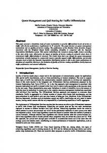
5. Numerical results In this section, we use the extensive numerical results to show the performance of Algorithm Greedy-OMCP. The Greedy-OMCP algorithm is denoted by G-OMCP, and is compared with the Kapproximation algorithm [19], (denoted by Greedy), and FPTAS OMCP [18] (denoted by OMCP). In the first group of results, we show the performances of the algorithms on well-know network topologies (ArpaNet, NSFNET, and ItalianNet). Here we present the results for ItalianNet because the results are similar. We use ∈ =0.1 for the polynomial time approximation scheme OMCP [18]. We observed that for all test cases, Greedy-OMCP always provides the best results among all algorithms, even better than the FPTAS OMCP. In Fig. 5, among the 100 connections, in 25% to 33% of the test cases (29% for the infeasible constraint, 33% for the tight constraint, and 25% for the loose constraint), the path computed by OMCP is better than the path computed by Greedy, in 25% to 34% of the test cases(29% for the infeasible constraint, 34% for the tight constraint, and 25% for the loose constraint), the path computed by G-OMCP is better than the path computed by Greedy. The paths computed by Greedy are always outperformed by the paths computed by both OMCP and G-OMCP. In Fig. 6, we show the qualitative comparison of the performances of G-OMCP and Greedy. Because OMCP is a theoretically proved scheme, we still use the length of the path found by OMCP as , where the standard for normalization. For any path p, its relative error is calculated as pOMCP is the path found by OMCP for the source destination pair. For each of these two algorithms, its relative error is the average of relative errors of all 100 paths computed by the algorithm. In Fig. 6, we can see that G-OMCP has noticeably lower relative errors than Greedy for all scenarios. For example, for the tight constraint, Greedy computed paths that are 4.3% worse than the paths computed by OMCP, while the paths computed by G-OMCP is even better than those computed by OMCP.
Figure 5. Comparison of better paths on ItalianNET
Figure 6. Comparison of path lengths on ItalianNET
Next, we compare the running times between the OMCP, G-OMCP and Greedy in Fig. 7. As we observed, the running time of G-OMCP is much shorter than the running time of OMCP, while the two algorithms computed paths with comparable lengths. The running times of Greedy and G-OMCP are comparable. For example, for the loose constraint, the average running time of Greedy is about 2 msecs, while the average running time of G-OMCP is around 11 msecs. But we can observe that GOMCP provides noticeable better path performances than Greedy does. Next, we use some large random topologies to evaluate the algorithms. Similarly, we used the network topology with 100 nodes with 390 edges generated by BRITE to verify the path performances of the algorithms. We observe, from Fig. 8, similar performances as in the case of ItalianNet. G-OMCP outperformed Greedy in 21% (infeasible constraint), 19% (tight constraint), 20% (loose constraint) of the test cases. We also observe from Fig. 9 that G-OMCP again outperformed Greedy in qualitative comparisons. Again, G-OMCP has similar performance as OMCP, but has a noticeable less running time in Fig. 10.
41
Multi-Constrained QoS Routing for Distraction-free Service in Pervasive Environment Weiyi Zhang, Jun Kong
Figure 7. Comparison of running Figure 8. Comparison of numbers of better time on ItalianNET paths on a large random network topology
Figure 9. Comparison of numbers of path lengths on a large random network topology
Figure 10. Comparison of running time on a large random network topology
Another very important metric is the maximum number of paths stored on a node, qmax. In the analysis of the running time, we know that qmax could be exponential. However, we observed from the results, which are shown in Fig. 11, that the value of qmax is not large in practice.
Figure 11. The maximum number of paths stored on the network nodes
Figure 12. Comparison of running times on ItalianNet
For example, for the ItalianNet, the maximum number of stored paths is 18 (infeasible constraint), 18 (tight constraint), and 20 (loose constraint). Meanwhile, even for the large random network, the maximum number of stored paths is no more than 23, (21 for the infeasible constraint, 23 for the tight constraint, 22 for the loose constraint). It worth noting that based on the observation from the simulation results, we can modify the Algorithm Greedy-OMCP to a polynomial-time algorithm by limiting the maximum number of paths which can be stored at a node. For example, based on the simulation results, we can expect to get an optimal solution or provide a very good solution in practice by setting qmax = 30, which means that there are at most 30 paths can be stored at a node. The next result is the running time comparison between the two algorithms for DMCP problem in the ItalianNet. In Fig. 12, as we expected, the running time of F-DMCP is longer than the time of Random algorithm. For example, when W = 40, the running times of Random are around 0.0025 seconds averagely, F-DMCP takes 0.3845 seconds. Although the running time of F-DMCP is longer, the time is still in the reasonable range. And the algorithm runs fast in practice. Another observation is that the running time of F-DMCP increases with the larger weight constraint. The reason is in that as
42
Journal of Next Generation Information Technology Volume 1, Number 2, August, 2010 the weight constraint is larger, the solution space will become larger as well. Therefore, we could store more paths in the queue Q, and consequently execute more necessary checks in the algorithm.
6. Related work Our work is related to the dynamic resource allocation in a pervasive environment. In order to provide a distraction-free service, a pervasive computing system needs to allocate resources dynamically based on resource variability. It is a challenging issue to select a set of applications to reach the maximum benefit [14, 17] and satisfy system and network constraints. Most researchers have considered the resource allocation and system reconfiguration at the application layer [2, 3, 12]. In order to achieve a global optimization, Zhang et al. [22] study the resource allocation at the application level and QoS routing at the network level together. Another related research topic is the MCP problem, which is NP-complete [15]. Due to its increasing important applications, this problem has been studied by many researchers. Along the line of provably good algorithms, Warburton in [16] first developed a fully polynomial time approximation scheme (FPTAS) [4] for the Delay Constrained Least Cost problem (DCLC) on an acyclic graph. Lorenz and Raz in [9] presented a fast FPTAS with a time complexity of O(mn(loglogn+ 1/ε)). In a recent paper [20], Xue et al. improved the result of [9] with a time complexity of O(mn(logloglogn+1/ε)). The algorithm of Xue et al. [20] is the fastest known approximation scheme for the DCLC problem on general graphs. Chen and Nahrstedt [1] studied the decision version of the DCLC problem and proposed a polynomial time heuristic algorithm based on scaling and rounding of the delay parameter [5, 13] so that the delay parameter of each edge is approximated by a bounded integer. Yuan [21] studied the decision version of the multi-constrained path problem, and presented a limited granularity heuristic and a limited path heuristic for this problem. The limited granularity heuristic can be viewed as a generalization of the heuristic of Chen and Nahrstedt [1] for the case with two additive constraints to the case with K additive constraints, and has a time complexity of O(mn(n/ε)K-1). In [20], Xue et al. studied the general DMCP problem and presented an O(m(n/ε)K-1) time algorithm which either finds a feasible solution or confirms that there does not exist a source-destination path whose first path weight is bounded by the first constraint and whose every other path weight is bounded by (1-ε) times the corresponding constraint. The algorithm of Xue et al. [20] improves that of Chen and Nahrstedt [1] and that of Yuan [21], and is the fastest known algorithm along this direction. In [18], Xue et al. studied OMCP, an optimization version of the multi-constrained path problem, and presented a simple Kapproximation algorithm based on the computation of a shortest path with respect to a single auxiliary edge weight function. Along the line of heuristic algorithms that perform well in practice but lack of proved theoretical performance guarantee, there is a very long list of publications. Korkmaz and Krunz [7] proposed RANDOM (a randomized heuristic) for the DMCP problem, which uses a simple necessary condition to reduce search space.
7. Conclusion In a pervasive environment, user mobility causes a dynamic change on interaction context. In order to provide a distraction-free service, which hides the fact of user mobility, one fundamental issue is to provide a QoS routing between a moving user and a service provider. This paper provides an exact algorithm for the routing issue. Simulation results prove the performance of our approach. In the future, we will combine the routing algorithm with the adaption at the application layer to provide a distraction-free service in a pervasive environment.
8. Acknowledgement This work is supported in part by ND EPSCoR State Seed Grants #FAR0015845 and #FAR0015846, and HP Labs Innovation Research Program (2009-1047-1-A).
43
Multi-Constrained QoS Routing for Distraction-free Service in Pervasive Environment Weiyi Zhang, Jun Kong
9. References [1] S. Chen, K. Nahrstedt, “On Finding Multi-Constrained Paths”, Proc. IEEE ICC'98, pp. 874-879, 1998. [2] S. Cheng, D. Garlan, B. Schmerl, J. P. Sousa, B. Spitznagel, P.Steenkiste, and N. Hu, “Software Architecture-based Adaptation for Pervasive Systems”, Proc. International Conference on Architecture of Computing Systems, 2002. [3] S. Cheng, A. Huang, D. Garlan, B. Schmerl, and P. Steenkiste, “Rainbow: Architecture-Based Self Adaptation with Reusable Infrastructure”, IEEE Computer, 37(10), pp. 46-54, 2004. [4] T.H. Cormen, C.E. Leiserson, R.L. Rivest, C. Stein, Introduction to Algorithms, MIT Press, 2001. [5] Ibarra, C.E. Kim, “Fast approximation algorithms for the knapsack and sum of subset problems”, Journal of the ACM 22, pp. 463-468, 1975. [6] J. M. Jaffe, “Algorithms for Finding Paths with Multiple Constraints”, Networks 14, pp. 95-116, 1984. [7] T. Korkmaz, M. Krunz, “A Random Algorithm for Finding a Path Subject to Multiple QoS Constraints”, Computer Networks 36(23), pp. 251-268, 2001. [8] D. Lorenz, A. Orda, D. Raz, Y. Shavitt, “Efficient QoS Partition and Routing of Unicast and Multicast”, Proc. IWQoS 2000, pp. 75-83, 2000. [9] D. Lorenz, D. Raz, “A simple efficient approximation scheme for the restricted shortest paths problem”, Operations Research Letters 28, pp.213-219, 2001. [10] Q. Ma, P. Steenkiste, “Quality-of-service routing for traffic with performance guarantees”, Proc. IWQoS'97, 1997. [11] B. Mukherjee, “WDM optical networks: progress and challenges”, IEEE JSAC, Vol. 18, pp. 1810-1824, 2000. [12] P. Oreizy, M. Gorlick, R. Taylor, D. Heimhigner, G. Johnson, N.Medvidovic, A. Quilici, D. Rosenblum, and A. Wolf, “An architecture based approach to self-adaptive software”, IEEE Intelligent Systems, 14(3), pp.54-62, 1999. [13] S. Sahni, “General techniques for combinatorial approximation”, Operations Research 25, pp.920-936, 1977. [14] S. Shenker, “Fundamental Design Issues for the Future Internet”, IEEE JSAC 13, pp. 1176-1188, 1995. [15] Z. Wang, J. Crowcroft, “Quality-of-service routing for supporting multimedia applications”, IEEE JSAC 14, pp.1228-1234, 1996. [16] A. Warburton, “Approximation of Pareto optima in multiple-objective, shortest path problem”, Operations Research 35, pp. 70-79, 1987. [17] Z. Wu and Q. Yin, “A Heuristic for Bandwidth Allocation and Management to Maximize User Satisfaction Degree on Multiple MPLS Paths”, IEEE CCNC’2006, pp.35-39, 2006. [18] G. Xue, A. Sen, W. Zhang, J. Tang, K. Thulasiraman, “Finding a path subject to many additive QoS constraints” IEEE/ACM ToN 15, pp. 201-211, 2007. [19] G. Xue and W. Zhang, “Multi-constrained QoS routing: Greedy is good”, Proc. IEEE Globecom, 2007. [20] G. Xue, W. Zhang, J. Tang, K. Thulasiraman, “Polynomial time approximation algorithms for multi-constrained QoS routing”, IEEE/ACM Transactions on Networking, pp.656-669, 2008. [21] X. Yuan, “Heuristic Algorithms for Multiconstrained Quality-of-Service Routing”, IEEE/ACM Transactions on Networking 10(2), pp.244-256, 2002. [22] W. Zhang, J. Kong, K. Nygard, and M. Li, “Adaptive Configuration of Pervasive Computing System with QoS Consideration”, Proc. 6th IEEE CCNC, 2009.
44