Multi-Dimensional Bitmap Indices for Optimising Data Access within

Multi-Dimensional Bitmap Indices for Optimising Data Access within Object Oriented Databases at CERN

Dissertation 26/11/2001

CERN-THESIS-2001-026

eingereicht von: Mag. Kurt Stockinger

zur Erlangung des akademischen Grades Doctor rerum socialium oeconomicarumque (Dr. rer. soc. oec.) Doktor der Sozial- und Wirtschaftswissenschaften

Fakult¨ at f¨ ur Wirtschaftswissenschaften und Informatik Universit¨ at Wien

Erstgutachter: ao.Univ.-Prof. Dr. Erich Schikuta Zweitgutachter: Univ.-Prof. Dr. Dr. Gerald Quirchmayr CERN Betreuer: Dr. Dirk D¨ ullmann

Genf, im November 2001

To Sabinka

Contents 1 Introduction 1.1 Multi-Petabyte Data Challenge at CERN 1.2 HEP Data Model . . . . . . . . . . . . . . 1.3 Physics Analysis . . . . . . . . . . . . . . 1.4 Contribution of the Thesis . . . . . . . . .

. . . .

. . . .

. . . .

. . . .

. . . .

. . . .

. . . .

. . . .

. . . .

. . . .

. . . .

. . . .

. . . .

. . . .

. . . .

. . . .

. . . .

. . . .

. . . .

. . . .

. . . .

9 10 10 11 12

2 “Conventional” Multi-dimensional Access Methods 2.1 Introduction . . . . . . . . . . . . . . . . . . . . . . . . 2.2 Problem Definition . . . . . . . . . . . . . . . . . . . . 2.3 Basic Data Structures . . . . . . . . . . . . . . . . . . 2.4 Point Access Methods (PAMs) . . . . . . . . . . . . . 2.4.1 Multi-Dimensional Hashing . . . . . . . . . . . 2.4.2 Hierarchical Access Methods . . . . . . . . . . 2.5 Spatial Access Methods (SAMs) . . . . . . . . . . . . 2.5.1 Overlapping Regions . . . . . . . . . . . . . . . 2.5.2 Clipping . . . . . . . . . . . . . . . . . . . . . . 2.5.3 Transformation . . . . . . . . . . . . . . . . . . 2.5.4 Multiple Layers . . . . . . . . . . . . . . . . . . 2.6 Pyramid-tree . . . . . . . . . . . . . . . . . . . . . . . 2.6.1 Treatment of Data Space . . . . . . . . . . . . 2.6.2 Index Creation and Query Processing . . . . .

. . . . . . . . . . . . . .

. . . . . . . . . . . . . .

. . . . . . . . . . . . . .

. . . . . . . . . . . . . .

. . . . . . . . . . . . . .

. . . . . . . . . . . . . .

. . . . . . . . . . . . . .

. . . . . . . . . . . . . .

. . . . . . . . . . . . . .

. . . . . . . . . . . . . .

. . . . . . . . . . . . . .

. . . . . . . . . . . . . .

. . . . . . . . . . . . . .

. . . . . . . . . . . . . .

14 14 14 15 16 16 17 17 18 21 22 24 24 25 26

3 Bitmap Indices 3.1 Introduction . . . . . . . . . . . . . . . . . . . . 3.2 Simple Bitmap Indices . . . . . . . . . . . . . . 3.2.1 Space Complexity . . . . . . . . . . . . 3.2.2 Time Complexity . . . . . . . . . . . . . 3.2.3 Pros and Cons of Simple Bitmap Indices 3.3 Equality, Range, Interval Encoding . . . . . . . 3.4 Range-Based Indices . . . . . . . . . . . . . . . 3.5 Encoded Bitmap Indices . . . . . . . . . . . . . 3.6 Miscellaneous Techniques . . . . . . . . . . . . 3.7 Bitmap Compression . . . . . . . . . . . . . . .

. . . . . . . . . .

. . . . . . . . . .

. . . . . . . . . .

. . . . . . . . . .

. . . . . . . . . .

. . . . . . . . . .

. . . . . . . . . .

. . . . . . . . . .

. . . . . . . . . .

. . . . . . . . . .

. . . . . . . . . .

. . . . . . . . . .

. . . . . . . . . .

. . . . . . . . . .

28 28 28 29 30 30 31 31 33 34 34

2

. . . . . . . . . .

. . . . . . . . . .

. . . . . . . . . .

. . . . . . . . . .

3.7.1 3.7.2 3.7.3

LZ Encoding . . . . . . . . . . . . . . . . . . . . . . . . . . . . . . . . . ExpGol Encoding . . . . . . . . . . . . . . . . . . . . . . . . . . . . . . . Byte-Aligned Bitmap Codes . . . . . . . . . . . . . . . . . . . . . . . . .

4 Current Access Methods for HEP 4.1 Introduction . . . . . . . . . . . . 4.2 Implementation Issues . . . . . . 4.3 Performance Analysis . . . . . . 4.4 Conclusions . . . . . . . . . . . .

Queries . . . . . . . . . . . . . . . . . . . . . . . .

. . . .

. . . .

. . . .

. . . .

. . . .

. . . .

. . . .

. . . .

. . . .

. . . .

. . . .

. . . .

. . . .

. . . .

. . . .

5 Bitmap Indices for Scientific Data 5.1 Introduction . . . . . . . . . . . . . . . . . . . . . . . . . . . . . . . . . 5.2 Bitmap Indices for HEP . . . . . . . . . . . . . . . . . . . . . . . . . . 5.3 Implementation on Objectivity/DB . . . . . . . . . . . . . . . . . . . . 5.4 Brief Justification of the Bitmap Index Approach . . . . . . . . . . . . 5.4.1 Cost Model for Equality Encoded Bitmap Indices . . . . . . . . 5.4.2 Size of the Index . . . . . . . . . . . . . . . . . . . . . . . . . . 5.4.3 I/O Complexity of the Index . . . . . . . . . . . . . . . . . . . 5.4.4 Maximal Page I/O Costs for Index Evaluation Phase . . . . . . 5.4.5 Page I/O Costs for Candidate Check Phase . . . . . . . . . . . 5.4.6 Total I/O Costs . . . . . . . . . . . . . . . . . . . . . . . . . . 5.5 Analytical Results . . . . . . . . . . . . . . . . . . . . . . . . . . . . . 5.5.1 Equality Encoding on Generic Tags . . . . . . . . . . . . . . . 5.5.2 Equality Encoding on Sliced Tags . . . . . . . . . . . . . . . . 5.5.3 Comparison - Equality Encoding Generic Tags vs. Sliced Tags 5.6 Partitioned Range Encoding . . . . . . . . . . . . . . . . . . . . . . . . 5.7 Conclusions . . . . . . . . . . . . . . . . . . . . . . . . . . . . . . . . . 6 Generic Range Encoding 6.1 Introduction . . . . . . . . . . . . . . . . . . . . . . . . . . . . 6.2 Example: Range Encoding for Non-Discrete Attribute Values 6.3 Generic Range Encoding - A Novel Algorithm . . . . . . . . 6.4 Cost Model for GenericRangeEncoded Bitmap Indices . . . . 6.4.1 I/O Complexity of the Index . . . . . . . . . . . . . . 6.4.2 Page I/O Costs for Index Evaluation Phase . . . . . . 6.4.3 Page I/O-Costs for Candidate Check Phase . . . . . . 6.5 Analytical Results . . . . . . . . . . . . . . . . . . . . . . . . 6.6 Experimental Results . . . . . . . . . . . . . . . . . . . . . . . 6.7 Analytical vs. Experimental Results . . . . . . . . . . . . . . 6.8 Conclusions . . . . . . . . . . . . . . . . . . . . . . . . . . . .

3

. . . . . . . . . . .

. . . . . . . . . . .

. . . . . . . . . . .

. . . . . . . . . . .

. . . . . . . . . . .

. . . .

. . . . . . . . . . . . . . . .

. . . . . . . . . . .

. . . .

. . . . . . . . . . . . . . . .

. . . . . . . . . . .

. . . .

. . . . . . . . . . . . . . . .

. . . . . . . . . . .

. . . .

. . . . . . . . . . . . . . . .

. . . . . . . . . . .

35 35 36

. . . .

39 39 40 41 43

. . . . . . . . . . . . . . . .

44 44 44 45 46 47 48 49 49 50 50 53 53 55 57 57 60

. . . . . . . . . . .

61 61 61 63 68 68 69 69 71 74 77 79

7 Advanced Features 7.1 Introduction . . . . . . . . . . . . . . . . . . . . . . . . . . . . . . . . . 7.2 Adaptive Index . . . . . . . . . . . . . . . . . . . . . . . . . . . . . . . 7.3 Binning Strategies . . . . . . . . . . . . . . . . . . . . . . . . . . . . . 7.4 Bitmap Compression on Uniformly Distributed Data . . . . . . . . . 7.4.1 Equality Encoded Bitmap Index . . . . . . . . . . . . . . . . . 7.4.2 Range Encoded Bitmap Index . . . . . . . . . . . . . . . . . . . 7.4.3 Compressed Equality Encoding vs. Verbatim Range Encoding 7.5 Bitmap Compression on Non-Uniformly Distributed Data . . . . . . . 7.6 Conclusions . . . . . . . . . . . . . . . . . . . . . . . . . . . . . . . . . 8 Applications 8.1 Introduction . . . . . . . . . . . . . . . . . . . 8.2 Extended Cost Model . . . . . . . . . . . . . 8.2.1 Clustering . . . . . . . . . . . . . . . . 8.2.2 Correlation . . . . . . . . . . . . . . . 8.3 Query Parser . . . . . . . . . . . . . . . . . . 8.4 High Energy Physics . . . . . . . . . . . . . . 8.4.1 Data Distribution . . . . . . . . . . . 8.4.2 Sample Queries . . . . . . . . . . . . . 8.4.3 Comparison with the Cost Model . . . 8.4.4 Bitmap Compression . . . . . . . . . . 8.5 Astronomy . . . . . . . . . . . . . . . . . . . 8.5.1 Data Preparation . . . . . . . . . . . . 8.5.2 “Typical” Astronomy Sample Queries 8.5.3 Analysis of the Results . . . . . . . . . 8.6 Conclusions . . . . . . . . . . . . . . . . . . .

. . . . . . . . .

. . . . . . . . .

. . . . . . . . .

. . . . . . . . .

. . . . . . . . .

80 80 80 81 81 81 83 84 86 90

. . . . . . . . . . . . . . .

. . . . . . . . . . . . . . .

. . . . . . . . . . . . . . .

93 93 93 93 94 94 95 95 96 99 100 101 102 103 105 107

9 Outlook - Query Optimisation in a Grid Environment 9.1 Introduction . . . . . . . . . . . . . . . . . . . . . . . . . . . . . . . . . . . . 9.2 The EU DataGrid . . . . . . . . . . . . . . . . . . . . . . . . . . . . . . . . 9.3 Optimisation Opportunities for Analysis . . . . . . . . . . . . . . . . . . . . 9.4 Grid Query Optimisation for Analysis within a Typical Grid Architecture . 9.4.1 The Local Application Layer . . . . . . . . . . . . . . . . . . . . . . 9.4.2 The Grid Application Layer . . . . . . . . . . . . . . . . . . . . . . . 9.4.3 The Collective Services Layer . . . . . . . . . . . . . . . . . . . . . . 9.4.4 The Task of Grid Query Optimisation within a Typical Architecture 9.5 Interaction of Services for a Particular HEP Use Case . . . . . . . . . . . . 9.6 Conclusions and Future Work . . . . . . . . . . . . . . . . . . . . . . . . . .

. . . . . . . . . .

. . . . . . . . . .

108 108 108 108 111 112 112 113 114 115 117

. . . . . . . . . . . . . . .

. . . . . . . . . . . . . . .

. . . . . . . . . . . . . . .

. . . . . . . . . . . . . . .

. . . . . . . . . . . . . . .

. . . . . . . . . . . . . . .

. . . . . . . . . . . . . . .

. . . . . . . . . . . . . . .

. . . . . . . . . . . . . . .

. . . . . . . . . . . . . . .

. . . . . . . . . . . . . . .

. . . . . . . . . . . . . . .

. . . . . . . . . . . . . . .

. . . . . . . . . . . . . . .

. . . . . . . . . . . . . . .

. . . . . . . . . . . . . . .

10 Conclusions

118

11 Acknowledgements

120

4

List of Figures 1.1

Particle traces after event collision. . . . . . . . . . . . . . . . . . . . . . . . . .

12

2.1 2.2 2.3 2.4 2.5 2.6 2.7 2.8 2.9 2.10

R-tree. . . . . . . . . . . . . . . . . . . . . . . . . . . R*-tree. . . . . . . . . . . . . . . . . . . . . . . . . . X-tree. . . . . . . . . . . . . . . . . . . . . . . . . . . Various shapes of the X-tree in different dimensions. R+-tree. . . . . . . . . . . . . . . . . . . . . . . . . . Hilbert Curves of order 1, 2 and 3. . . . . . . . . . . Hilbert R-tree. . . . . . . . . . . . . . . . . . . . . . Space partitioning method of the Pyramid-tree. . . . Key values for the Pyramid-tree. . . . . . . . . . . . Query processing with the Pyramid-tree. . . . . . . .

. . . . . . . . . .

19 21 22 22 23 24 25 26 26 27

3.1 3.2 3.3

Algorithm RangeEval and RangeEval-Opt. . . . . . . . . . . . . . . . . . . . . Hufmann encoded bitmap index. . . . . . . . . . . . . . . . . . . . . . . . . . . Compression ratios of various bitmap compression algorithms. Bit desity (xaxis) vs. compression ratio (y-axis). . . . . . . . . . . . . . . . . . . . . . . . . Time for compression and uncompression of various bitmap compression algorithms. . . . . . . . . . . . . . . . . . . . . . . . . . . . . . . . . . . . . . . . . . Compression algorithm with best performance on Boolean operations. . . . . .

33 34

3.4 3.5 4.1 4.2 5.1 5.2 5.3 5.4 5.5 5.6

. . . . . . . . . .

. . . . . . . . . .

. . . . . . . . . .

. . . . . . . . . .

. . . . . . . . . .

. . . . . . . . . .

. . . . . . . . . .

. . . . . . . . . .

. . . . . . . . . .

. . . . . . . . . .

. . . . . . . . . .

. . . . . . . . . .

. . . . . . . . . .

. . . . . . . . . .

Response times for selecting attributes based on various different tag implementations. a) 81,060 tags with 302 attributes b) 1,000,000 tags with 25 attributes. Access patterns of disk head movements for reading parallel streams a) without prefetch optimsation b) with prefetch optimisation. . . . . . . . . . . . . . . . . One sided-range query on a range encoded bitmap index. . . . . . . . . . . . . Architectural overview of the bitmap index on top of Objectivity/DB. . . . . . Variable query selectivities for two sided-range queries. . . . . . . . . . . . . . . Access granularity of a database in terms of pages rather than objects. . . . . . Generic tag - I/O costs for optimal number of bins for 50% attribute selectivity (worst case) compared to sequential scan. . . . . . . . . . . . . . . . . . . . . . Generic tag - I/O costs for optimal number of bins for 50% attribute selectivity (worst case) are split into index-I/O and candidate-I/O. . . . . . . . . . . . . .

5

37 37 38 42 42 45 46 48 50 54 55

5.7

Generic tag - I/O costs for multiple attribute selectivities compared to sequential scan. . . . . . . . . . . . . . . . . . . . . . . . . . . . . . . . . . . . . . . . . . . 5.8 Sliced tag - I/O costs for optimal number of bins for 50% attribute selectivity (worst case) compared to sequential scan. . . . . . . . . . . . . . . . . . . . . . 5.9 Sliced tag - I/O costs for optimal number of bins for 50% attribute selectivity (worst case) are split into index-I/O and candidate-I/O. . . . . . . . . . . . . . 5.10 Sliced tag - I/O costs for multiple attribute selectivities compared to sequential scan. . . . . . . . . . . . . . . . . . . . . . . . . . . . . . . . . . . . . . . . . . . 5.11 Partitioned Equality Encoding (EQ) vs. Partitioned Range Encoding (Range). 6.1 6.2 6.3 6.4 6.5 6.6 6.7 6.8

One-sided range query on a range encoded bitmap index. . . . . . . . . . . . . Candidate check in multi-dimensional space. For each attribute the candidates are checked separately. . . . . . . . . . . . . . . . . . . . . . . . . . . . . . . . . Analytical results: Page I/O for queries over multiple dimensions with various selectivities. 10 bins. . . . . . . . . . . . . . . . . . . . . . . . . . . . . . . . . . Analytical results: Page I/O for queries over multiple dimensions with various selectivities. 100 bins. . . . . . . . . . . . . . . . . . . . . . . . . . . . . . . . . Analytical results: Page I/O for queries over multiple dimensions with various selectivities. 1,000 bins. . . . . . . . . . . . . . . . . . . . . . . . . . . . . . . . Analytical results: Page I/O for queries over multiple dimensions with various selectivities. 1,000,000 bins. . . . . . . . . . . . . . . . . . . . . . . . . . . . . . Experimental results: Page I/O and response for queries over multiple dimensions with various selectivities - one to three dimensions. . . . . . . . . . . . . . Experimental results: Page I/O and response for queries over multiple dimensions with various selectivities - five to 25 dimensions. . . . . . . . . . . . . . .

Query response time of verbatim vs. compressed equality encoded bitmap index - 100 bins. . . . . . . . . . . . . . . . . . . . . . . . . . . . . . . . . . . . . . . . 7.2 Query response time of verbatim vs. compressed equality encoded bitmap index - 1000 bins. . . . . . . . . . . . . . . . . . . . . . . . . . . . . . . . . . . . . . . 7.3 Compression ratio of range encoded bitmap index with 100 bins. . . . . . . . . 7.4 Query response time for compressed equality encoding vs. verbatim range encoding. . . . . . . . . . . . . . . . . . . . . . . . . . . . . . . . . . . . . . . . . . 7.5 Query response time for compressed equality encoding vs. verbatim range encoding. . . . . . . . . . . . . . . . . . . . . . . . . . . . . . . . . . . . . . . . . . 7.6 Range encoded bitmap index based on data following an exponential distribution. 7.7 Response time for verbatim vs. compressed bitmap indices. Queries include the “”-operator. . . . . . . . . . . . . . . . . . . . . . . . . . . . . . . . . . . . . . 7.9 Response time for compressed bitmap indices. Queries including “”-operator. . . . . . . . . . . . . . . . . . . . . . . . . . 7.10 Response time for queries based on compressed bitmap index with 100 bins vs. 400 bins. Queries include the “ 100.5) AND (pT1 < 83.7) AND (pT2 < 92.6) where Energy, pT1 and are pT2 experiment specific physics parameters. An example of a detector image which traces the paths of particles after the collision is given in Figure 1.1. In a typical analysis effort, the number of resulting events, i.e. the found set, is iteratively reduced by applying cuts with smaller ranges or by adding more attributes to the cuts which results in a higher dimensional query. The results yielded by the cuts are mostly stored in histograms and plotted afterwards for analysing the physics properties. During other typical analysis efforts, arbitrary mathematical expressions of attributes can be used during the selection. A typical example looks like: sin(pT1) > 0.7 OR sin(pT1) > 0.3 Currently, data access methods in HEP are based on sequentially scanning a search space up to several hundred of dimensions. 11

Figure 1.1: Particle traces after event collision.

1.4

Contribution of the Thesis

In Chapter 2 we give an overview of the main trends in database access methods of the last three decades of research. We define the basic terminology we use throughout the thesis and categorise the index data structures according to hash-based and interval-based structures. We also discuss point access and spatial access methods with respect to high-dimensional search spaces. Trends in the state of the art of bitmaps indices which are more recent multi-dimensional index data structures mainly applied in data warehouse applications are presented in Chapter 3. We discuss different bitmap design strategies for optimising various query types. We also review various bitmap compression techniques for reducing the size of the index and also improving the query performance characterstics. Chapter 4 is dedicated to an evaluation of some of the current access methods in High Energy Physics (HEP) for end-user analysis. We give a performance analysis of sequentially scanning physics data clustered in two different ways on top of an object oriented database management system. The two different clustering approaches are called generic tag and sliced tag. The results of this analysis serve as the main comparison for evaluating multi-dimensional access methods. In Chapter 5 we report on the desgin and implementation of bitmap indices for scientific data which is characterised by non-discrete attribute values, in particular mostly floating points. We start with a brief justification that bitmap indices can improve the query response time of

12

typical physics analysis queries. We will introduce a novel cost model for studying analytically the performance of so-called equality encoded bitmap indices and discuss the optimal index size for various kinds of queries. In Chapter 6 we propose a novel bitmap index algorithm called GenericRangeEval for processing multi-dimensional range queries against scientific data. We also extend the cost model introduced in Chapter 5 to predict the performance of this index data structure. Both analytically and experimentally we show that for up to 25 dimensional range queries our proposed bitmap index can significantly speed up the query responds time when compared to the sequential scan. Various optimisation possibilities for bitmap indices are discussed in Chapter 7. In particular, we elaborate on different binning strategies and different query plans. We also evaluate experimentally the impact of bitmap compression for equality encoded and range encoded bitmap indices based on scientific data. In Chapter 8 we demonstrate that by using this kind of access method we can significantly improve the performance of typical queries of two different application areas, namely High Energy Physics and Astronomy. Chapter 9 is dedicated to an outlook of Grid Query Optimisation where we discuss various access optimisation opportunities within a wider range of HEP data. In particular, we elaborate on optimisation opportunies for possible physics analysis on data which is replicated all over the world. Concluding remarks and a summary of the results of this thesis are given in Chapter 10.

13

Chapter 2

“Conventional” Multi-dimensional Access Methods 2.1

Introduction

In this chapter we first give a definition about the terminology for index data structures and then outline the main trends of data access methods in database management systems. Rather than giving a detailed discussion on every single algorithm, we will focus our attention on the most important data structures and give a short impression why some of these are still regarded as “near optimal” due to 30 years of intensive database research. One example of these data structures is the B-tree which was developed in 1972 by Bayer et al. [3] and is still regarded as one of the most universal algorithms. This will become clear when we take a closer look at Berchtold’s Pyramid-tree [5], a structure for indexing high-dimensional data where the basic idea is based on a simple B-tree.

2.2

Problem Definition

Before we start describing different kinds of index data structures, we define the terminology we will use throughout the thesis. Basically, we can distinguish between two classes of queries, namely: • Exact match queries of the form A = v where A refers to the attribute and v to a specific attribute value, e.g. income = ”30,000” • Range queries of the form v1 ≤ A ≤ v2 , e.g. 30,000 ≤ income ≤ 40,000. Throughout the thesis we will analyse access methods for improving the response time of so-called ad-hoc queries, i.e. interactive queries, over a multi-dimensional search space which is also called universe. In physics terminology a query is mostly referred to as a cut. For most of our evaluations the selectivity of a query has an impact on the performance of the data structure. We define the selectivity as the number of objects fulfilling the query constraint (result set) divided by the total number of objects. 14

For multi-dimensional queries we also talk about attribute query selectivity. In this case we refer to the selectivity of a particular attribute. Consider the following two dimensional query with a search space in the range [0;100] and uniformly distributed data values: a0 ≤ 30 AND a1 ≤ 20. In this case, the attribute query selectivity of a0 and a1 is 30% and 20% respectively. The total query selectivity is 6% (0.3 * 0.2 = 0.06). Especially during the discussing of so-called “conventional index data structures” we will often use the term bucket which refers to data points that are organised on one disk page.

2.3

Basic Data Structures

According to [43] we can use two different classifications for index data structures, namely: • Hash-based data structures and • Interval-based data structures. Typical hash-based data structures are: • Linear Hashing [46] • Extendible Hashing [21] Linear hashing divides the universe into binary intervals where an interval corresponds to a bucket. If the capacity of a bucket is reached, the bucket is split and a new entry is created in an overflow page [46]. Extendible Hashing maintains no overflow pages but a central directory. Each bucket (cell) has an entry in a directory. Once the capacity of the directory is reached, all cells are split which means that the directory doubles in size. Some of the most basic so-called interval-based structures are: • B-tree [3] • k-d-tree [4] • Quadtree [57] All of these data structures organise the data in a hierarchical way. A B-tree is a balanced tree with a height of log(n) where n is the number of nodes in the tree. The search operation on a B-tree is analogous to a search on a binary tree with an order of O(log(n)). The k-d-tree is a binary search tree that represents a recursive subdivision of the universe into subspaces by means of (d − 1) dimensional hyperplanes. One of the disadvantages of the k-d-tree is that the structure is sensitive to the order in which that data values are inserted and the data points are scattered all over the tree. Thus, variants of the k-d-tree use a split strategy that each hyperplane contains the same number of elements. However, for certain distributions no hyperplane can be found that splits the data points evenly [25]. The Quadtree is closely related to the k-d-tree and also decomposes the universe by means of iso-oriented hyperplanes. However, the Quadtrees are no binary trees any more. The intervalshaped partitions do not have to be of equal size and thus this tree is not necessarily well balanced. 15

Many of the more recent index data structures are based on these approaches. Thus, a good understanding of these basic techniques is vital for elaborating on more complicated multi-dimensional index data structures.

2.4

Point Access Methods (PAMs)

In the previous section we were discussing data structures which are mainly designed for main memory applications (apart from the B-tree) and, thus, do not bear in mind secondary or even tertiary storage devices. However, since database applications become more complex and the data volume much bigger, for instance at CERN we are dealing with data volumes up to several Petabytes, data structures must bear in mind both secondary storage and the underlying operating system. Point Access Methods can be categorised based on following strategies: • Multi-dimensional hashing • Hierarchical access methods As we mentioned already before, we will only discuss a few point access methods and have a closer look at them. Lets us start with typical data structures based on multi-dimensional hashing.

2.4.1

Multi-Dimensional Hashing

The Grid File The Grid File [45] is a typical data structure that is based on hashing. In short, a d-dimensional orthogonal non-regular grid makes up the universe of the data. The cells, which are yielded by putting a grid over all data, may have different shapes and sizes. These cells are associated with data buckets that in turn reside on one disk page. The grid itself is kept in main memory to guarantee that the data is found with two disk accesses at most. Data is retrieved according to the following two steps. First, the data is located in the cells by means of scales. Second, if the data does not reside in main memory, it must be fetched with a second disk access. The main disadvantage and, thus, a driving force for further research is the super linear directory growth for non-uniformly distributed data. Some variations of the Grid File are: • EXCELL (Extendible Cell) [70] • Two-Level Grid File [30] • Twin Grid File [36] EXCELL decomposes the universe in a regular way such that all grid cells are of equal size. The Two-Level Grid File uses a second grid file to manage the grid directory, the same is true for the Twin Grid File. However, the first one uses a hierarchical approach whereas the latter one uses a somewhat more balanced approach. A clustering approach based on grid files is presented in [59]. 16

2.4.2

Hierarchical Access Methods

We will now discuss a few of the most important hierarchical point access methods such as: • k-d-B tree [56] • LSD-tree [28] • Buddy-tree [62] • hB-tree [47] • BV-tree [23] The k-d-B tree partitions the universe like the adaptive k-d-tree with mutually disjoint regions. In addition it has the advantage of a B-tree, namely it is well balanced and thus guarantees the same access time for all data points. However, this structure does not guarantee minimal space utilisation due to the forced split policy [25]. The LSD-tree (Local Split Decision) partitions the universe like the adaptive k-d-tree with the advantage that it adapts well to non-uniformly distributed data values. The Buddy Tree can be regarded as an hybrid approach since it combines a dynamic hashing approach with a tree structured directory. In order to avoid the disadvantage of the Grid-file, the universe is partitioned into two parts of equal sizes with iso-oriented hyperplanes. The hB-tree (holey brick tree) uses the k-d-tree to organise the space. However, splitting is based on multiple attributes and so called “cascading” splits are avoided. Finally, the BV-tree is an attempt to solve the d-dimensional B-tree problem which can be regarded as a generalisation of the B-tree for higher dimensions. For further details, we refer to the respective literature.

2.5

Spatial Access Methods (SAMs)

In this section we discuss data structures which handle objects with spatial extension with complex structures that might be dynamic and large. According to [25] SAMs are modified PAMs which can be defined according to four categories: • Overlapping Regions (object bounding) • Clipping (object duplication, no overlap) • Transformation (object mapping to higher dimensional space) • Multiple layers (special case of overlapping regions)

17

2.5.1

Overlapping Regions

R-tree Let us start our discussion with the type Overlapping Regions where we will in particular focus our attention on one the most studied and modified trees, namely the R-tree which was first published by Guttman in 1984 [27]. The motivation for the development of the R-tree was the lack of flexibility of conventional data structures (hash tables, B-trees,...) in terms of multi-dimensional applications and spatial objects. Other structures like the Quadtree and the k-d-tree do not take paging of secondary memory into account whereas the k-d-B-tree bears this in mind but is most efficient for point data [27]. Thus, the need for the development of an index structure which represents spatial data objects by intervals in several dimensions was prevailing and regarded as an alternative to Grid Files that handle non-point data by mapping each object to a point in a higher-dimensional space [45]. The R-tree is a completely dynamic index structure for n-dimensional spatial objects analogous to a B+-tree. What is more, insertions and deletions can be intermixed with queries. However, the major difference is the representation of the nodes and the organisation of splits. Let us start our discussion with the representation of leaf nodes first. Leaf nodes contain index record entries of the form (I, tuple − identif ier) where tuple identifier refers to a tuple in the database and I is an n-dimensional rectangle containing the spatial objects it represents. In contrast, non-leaf nodes contain entries of the form (I, child − pointer) where child-pointer is the address of another node in the tree and I covers all rectangles in the lower node’s entries [27]. Each node corresponds to a disk page if the structure is disk resident (persistent). The R-tree uses rectangles for organising the universe. Thus, the data space can consist of many different multi-dimensional geometrical shapes which can be more efficiently organised and approximated by a simple shape such as a bounding box which is true for R-trees. We will later see that other index structures use different shapes for organising the data space, for example, by means of spheres. In short, the most important property of this simple approximation is that a complex object is represented by a limited number of bytes [10]. It is clear that due to this approximation some data gets lost. However, the most important geometric properties like • the location of the object and • the extension of the object in each axis are preserved. The main features of an R-tree are as follows [27]: • The root has at least two children unless it is a leaf. • Every non-leaf node contains between m and M index records (entries, children) unless it is the root whereas M is the maximum number of entries that will fit into a node and 18

m is defined as m ≤ M 2 and specifies the minimum number of node entries. What is more, this index record (I, tuple-identifier) is the smallest record that spatially contains the n-dimensional data object. • Every leaf node contains between m and M children unless it is the root. • All leaves appear on the same level. The height of an R-tree tree containing N index records is given in the worst case by: HeightR-tree=ceil(log(mN )) with a worst case space utilisation of space-utilisationR-tree = m M. A typical R-tree structure and the geometric form it represents is shown in Figure 2.1. R7 m1

R1 m2

p7

m9

R6 m6

m10

R7 R8 R2

p9

p8

m7

p10 m4

m5

X

R4 R5 R6

m8

m3

R4

p2

p3 R5

p1

R1 R2 R3

R8

p6

m1 m2 p10 m10 p9 p1 m4 m3 m5 m7 m8 p2 p3 p4 p5 p6 m9 m6 p7 p8

p5 p4

R3

Figure 2.1: R-tree.

The only important feature we want to highlight here is that overlapping regions are allowed in R-trees. However, the main difference to the B+-trees is the organisation of space and the treatment of splits which is based on d-dimensional minimum bounding boxes MBBs. The main idea is that nodes should be split in such a way that the possibility of these splitted nodes to be split again in the near future is minimised [27]. Minimising the total area of the two covering rectangles after the split can yield this effect. Finally, we will give an example of a query, which illustrates one typical feature of an Rtree, namely the effect of overlapping regions. By looking at Figure 2.1 which illustrates an R-tree, we see that for retrieving the point X (which lies within the rectangles m5 and m7) from our universe, two path accesses are required. In particular, following paths are yielded: • R8− > R4− > m7 • R7− > R3− > m5 R*-tree According the Beckmann, Kriegel et al. [10] the heuristic optimisation of the area of enclosing rectangles in each inner node of an R-tree can be improved by a combined approach. In particular, the R*-tree incorporates a combined optimisation of area, margin and overlap of 19

each enclosing rectangle in the directory. The main advantage of the R*-tree over Guttman’s Rtree is that both, point and spatial data can be more efficiently retrieved in a high-dimensional universe. [10] propose to minimise the margin or overlap of the minimum bounding rectangles in the R-tree. Further considerations and, thus, driving forces for the creation of the R*-tree are as follows: • Why not optimise storage utilisation? • Why not minimise the margin or overlap and to optimise the storage utilisation? The main problem of the R-tree is that it is only based on the optimisation of one parameter, namely the size of the minimum bounding box (MBB). However, since the data rectangles in the universe may have different sizes and shapes in addition to a dynamic change of the size of directory rectangles, the solution, which is yielded by an R-tree, may only be sub-optimal. In order to overcome a further problem of the R-tree, namely that the directory rectangles which are chosen with respect to the MBB is no longer suitable to a good retrieval performance in the new situation, the R*-tree achieves dynamic reorganisation and, thus, dynamic adaption of the directory rectangle by means of forced reinsert [10]. In short, rather than constantly inserting new data points and splitting the nodes afterwards, some nodes are taken out of a particular rectangle and inserted in the tree where they suit best. Thus, the whole tree adapts to the newly inserted data much better. Experiments show that if a threshold value of p=30% of M is reached (where p refers to the number of points in a particular rectangle), this method of forced reinsert should be applied [10]. To sum up, the R*-tree has following features [10]: • Forced reinsert changes the entries between neighbouring nodes and thus decreases the overlap, which also improves the storage utilisation. • Fewer splits occur due to a dynamic restructuring process of the whole tree. • Due to reinsertion of outer rectangles of a node, the ideal shape of the directory rectangles is quadratic. A typical R*-tree is depicted in Figure 2.2. X-tree One motivation for the development of the X-tree (eXtended Tree) [9] was that the R*-tree, which was one of the most powerful index structures at that time, did not perform well for dimensions greater than five. What is more, due to the fact that overlapping bounding rectangles are allowed, these overlaps may increase even faster with the increasing number of dimensions. According to experiments of Berchtold et al. these overlaps may reach up to 90% if the number of dimensions exceeds five, which yields quite bad performance values. The X-tree tries to overcome these obvious drawbacks of an R*-tree for high-dimensional space and introduces the concept of supernodes. This new method can be regarded as internal 20

p7

R8 R7

m9

R9

m1

m6

m10 p9

m2 R2

p8

p10

R7 R8 R9

m7

R1

R3 m4

R3

R4

R5

R6

R5

m5

m8

m3 R1

R2

p2

p1

p6

p3

p1 m2 m1 p10m10 m4 m3 p9m7 p8 m9 m5 p2 m6 m8 p7 p3 p4 p5 p6

R6 p5

R4 p4

Figure 2.2: R*-tree.

nodes that expand as the number of dimensions increases and consequently reduces the space of overlaps by a certain node split algorithm. In particular, directory nodes are extended over the usual block size, which in the worst case can be regarded as a linear scan. We can distinguish between two special cases of the X-tree [9]: • None of the directory nodes (internal nodes) is a supernode. • The directory consists of only one large supernode (root). In the first case, the X-tree can be regarded as a fully hierarchical index structure, which is very similar to an R-tree. This case is true for low-dimensional and non-overlapping data. The second case occurs for high-dimensional data and, thus, yields a performance which is equivalent to a linear directory scan which in turn is much more favourable than scanning data in a random fashion on disk and, thus, causing a high number of disk arm movements. A typical X-tree is depicted in Figure 2.3. The shape for different number of dimensions is given in Figure 2.4.

2.5.2

Clipping

A further technique of SAM is called Clipping. The main difference to Overlapping Regions is that no overlaps in the bounding rectangles are allowed. In other words, all bucket regions are mutually disjoint. R+-Tee The R+-tree [64] is a variant of Guttman’s R-tree and does not allow overlapping regions. This can be achieved by allowing partitions to split rectangles so that this technique results in zero overlap among intermediate node entries. However, avoiding overlap is only achieved at the expense of space, which increases the height of the tree. Due to the fewer number of access paths in comparison to an R-tree, the R+-tree yields better search performance for point queries [64]. Exact match queries in R+-trees correspond to single-path tree traversals 21

Figure 2.3: X-tree.

Figure 2.4: Various shapes of the X-tree in different dimensions.

from the root to one of the leaves. Range queries, on the other hand, lead to the traversal of multiple paths in both the R+-tree and the R-tree. A typical R+-tree is depicted in Figure 2.5.

2.5.3

Transformation

Let us explain this category of spatial access methods by means of Space Filling Curves, [22] which are used for representing extended objects by a list of grid cells or a list of one-dimensional intervals. In short, space filling curves try to store points, which are close in space, i.e. logical order, also close on disk, i.e. physical order. To put it in other words, these methods try to produce a physical order to points, which are very close in terms of logical order.The main idea is to visit all points in a grid without crossing itself. Hilbert R-tree The basic idea of the Hilbert R-tree [41] is to make use of the deferred splitting approach used in R-trees. In particular, an ordering of tree nodes is used which groups similar rectangles 22

p7 R9

R10 m1

m9

p9

p8

R2 p10 R7 m4 R1

R10R11R9

m6

m10 m2

m7

R3

R1 R2

m5 m3

p1

R4 R8 R6

R7 R3 R5

R5 R8 p2

m8

p1 p10 m2 m1 m5 p2 m8 p3 p4 p5 p6 m5 m5 m7 p8 m9m8 p7 m6 m10 p9 m4 m3

p6 p3 R6

R4 p4

p5 R11

Figure 2.5: R+-tree.

together and thus minimises the area and the perimeter of the resulting minimum bounding rectangles (MBRs). The authors of [41] claim that the Hilbert R-tree achieves higher space utilisation than the R*-tree proposed in [9] because latter does not allow to control space utilisation. In contrast, the Hilbert R-tree allows to adjust the splitting policy, e.g. 2-to-3 or 3-to-4 etc., which can result in 100% space utilisation, however, the average case is about 70%. The performance of R-trees depends on the algorithms, which cluster the data rectangles to nodes. The Hilbert R-tree uses the Hilbert Curve for clustering data. Let us first provide a brief introduction to the Hilbert Curve before we start our discussion on the Hilbert R-tree. Figure 2.6 shows a typical Hilbert Curve on a 2x2 grid, denoted by H1. It also shows different orders of the Hilbert Curves, which can be generalised for higher dimensionalities. In this case, the order tends to infinity where the result is a fractal. To sum it up, this kind of space-filling curve imposes a linear ordering on the grid points according to a fractal. For more details, we refer to [22]. We can now specify the main characteristics of a Hilbert R-tree [41]: • behaves like an R-tree • supports deferred splitting on insertion by means of the Hilbert value of the inserted data rectangle as the primary key What is more, for every node n of the tree, the • MBR and • Largest Hilbert Value (LHV) of the data rectangles that belong to the subtree with root n are stored. We see that similar to the R*-tree, overlapping regions are allowed. However, even non-leaf nodes contain entries about the LHVs. In our example we see that every node keeps track of the LHV and the MBR defined by XL, YL, XH, and YH, i.e. the coordinates of the MBR. 23

1

5

6

4

7

9

8

10

11

2 3

3

0

H

1

0

2

1

13

12

14

15

H

H

2

3

Figure 2.6: Hilbert Curves of order 1, 2 and 3.

One of the advantages of this splitting strategy over the R*-tree is that a shallower tree and a higher fanout are yielded due to a better packing mechanism of the tree [41].

2.5.4

Multiple Layers

The multiple layer technique can be regarded as a variant of the overlapping region approach, because data regions of different layers may overlap. The characteristics of this method can be summarised as follows [25]: • Layers are organised in a hierarchical way. • Each layer partitions the universe in a different way. • Data regions with a layer are disjoint. • Data regions do not adapt to the spatial extensions of the corresponding data objects. To give only some examples of the multiple layer technique, we want to mention the MultiLayer Grid File [65] and the R-File [37] and refer the reader again to the original literature for a detailed discussion.

2.6

Pyramid-tree

The motivation for the development of the Pyramid-tree was the sub-optimal split strategy of index structures studied so far. This is especially true for high-dimensional data. What is more, random page accesses for performing queries against a multi-dimensional universe mostly causes many disk arm movements and yields the typical I/O bottleneck. The Pyramid-tree tries to overcome these drawbacks by a new splitting strategy, which is optimised for high-dimensional data. The basic idea is to transform the d-dimensional data points into 1-dimensional values [5] and then store and access the data in a way, which we know from conventional B+-trees [17] and thus ”inherit” the positive features of this index data structure, namely: • height-balancing due to good splitting technique

24

(100, 100)

II

(30,75)

(51,75)

(55,75)

X [98] X

[92]

(35,65)

(20,60)

[107] I

(55,50)

(80,40)

III

(35,40)

X

[107] (45,35)

(20,38)

[206] [33]

(50,10) (3,5) (0,0)

LHV 33

I

XH YH

XL 3

YL 5

XH YH 35 40

LHV 107

LHV 34.5) ... } It is important to note that T agAttribute is a transient class which keeps a pointer to the underlying persistent-capable tag class. What is more, all objects of the type T agAttribute can be treated in the same way like C++ data types and can thus be used within complex mathematical expressions. After creating a tag collections, a simple analysis program looks like follows: HepExplorable *myTag = HepExplorable::findExplorable(name);

40

// define all fields that belong to genTag TagAttribute eventNo (myTags,"eventNo"); TagAttribute jet1E (myTags,"jet1E"); TagAttribute jet2E (myTags,"jet2E"); TagAttribute jet1Phi (myTags,"jet1Phi"); TagAttribute jet1Theta (myTags,"jet1Theta"); for(int more = myTag->start(); more ; more = myTag->next()) { // apply some cuts on jet1Phi and jet1Theta double jetE = 4; const double sinThetaCut = 0.9; if ( jet1E > jetE && jet2E < -jetE && fabs(sin(jet1Theta)) < sinThetaCut ) ... } The example above shows the usage of the generic tag. Since the interfaces for the sliced tag are the same, it can be used in the same way after replacing following statement during the creating of the tag: HepExplorableGenericTags myTags; is replaced by: HepExplorableSlicedTags myTags;

4.3

Performance Analysis

Our basic implementation of sliced tags in HepODBMS shows a very similar behaviour to the results presented in [54]. However, by using prefetch optimisation (read-ahead), the relative performance of the sliced tag is improved by a factor of two. Thus, the sliced tag is more efficient than the generic up to an attribute selectivity of 25% (i.e. 25% of all attributes of a tag are accessed) rather than 10% without prefetch optimisation. (We give a brief description of the prefetch optimisation below.) What is more, in the worst case, the sliced tag is only 2.5 times slower than the generic tag. Figure 4.1 a) shows the response time of accessing various numbers of tag attributes based on generic tags, “basic” sliced tags and sliced tags with prefetch optimisation. All our tests were performed at Caltech’s ”tier2b” machine (Dual 933 MHz Pentium III Linux server, 900 MB RAM, using a 600 GB 3ware RAID 0 array). We based our prefetch optimisation on findings presented in [31]. In short, rather than fetching single database pages of parallel data streams, i.e. multiple attributes, we prefetch multiple database pages in chunks of 1 MB. The advantage of this approach over fetching 41

140

120

120

100

100 Response time [sec]

Response time [sec]

140

80

60

80

60

40

40

20

20

0 a)

0

100 200 Number of acccessed attributes

Generic tag Sliced tag Sliced tag with prefetching

0

300 b)

0

5 10 15 20 Number of acccessed attributes

25

Figure 4.1: Response times for selecting attributes based on various different tag implementations. a) 81,060 tags with 302 attributes b) 1,000,000 tags with 25 attributes.

single database pages is the reduced number of disk head movements for random access and consequently reduced response times. Figure 4.2 shows the typical pattern of the disk arm for random access of two parallel streams without a) and with b) prefetch optimisation.

Figure 4.2: Access patterns of disk head movements for reading parallel streams a) without prefetch optimsation b) with prefetch optimisation.

We also carried out some performance benchmarks for 1,000,000 tags with 25 attributes. In this case, the advantage of sliced tags over generic tags is even more significant (see Figure 4.1 b). The sliced tag outperforms the generic tag up to an attribute selectivity of 80%. This is due to the bad performance of Objectivity for handling small objects such as the generic tag with 25 attributes.

42

4.4

Conclusions

In this chapter we demonstrated the performance of accessing typical physics tags which are clustered in two different ways. We gave a simple example in order to demonstrate a typical physics analysis code and compared the performance of the two clustering strategies. The sliced tag (attribute-wise clustering) with prefetching is ”optimal” up to 25% attribute selectivity - above this threshold the generic tag (object-wise clustering) performs better. In short, for large tags with many attributes the sliced tag is to be preferred if only a subset (up to 25%) of the attributes is selected. However, since tags for physics analysis will consist of some 1000 attributes whereas only up to a few tens will accessed at the same time, the sliced tag is clearly the better choice of implementation.

43

Chapter 5

Bitmap Indices for Scientific Data 5.1

Introduction

As we pointed out in the introductory chapter, currently most access methods in High Energy Physics analysis are based on sequentially scanning a multi-dimensional search space. Experiences from the past show that often the result set of the analysis is quite small and thus there is a good chance to improve the performance by applying a suitable multi-dimensional index data structure to prune the search space. We therefore propose using bitmap indices, which are optimised for processing complex multi-dimensional ad-hoc queries in read-mostly environments. [14] [15] [74] studied different kinds of bitmap encoding techniques but only for discrete values. However, additional complexity is imposed on the design and implementation of bitmap indices for non-discrete values since different optimisation techniques to the ones proposed so far have to be applied. In this chapter we will introduce a novel cost model for analysing the I/O costs for evaluating equality-encoded bitmap indices based on non-discrete attribute values. In particular, we will apply bitmap indices for high performance physics experiments and show that traditional physics analysis can be considerably improved by bitmap indices. By means of the cost model, we will analytically study the optimal number of bins, and thus the optimal size of multi-dimensional bitmap indices. In particular we will evaluate equalityencoded bitmap indices based on so-called generic tags and compare them to the performance of so-called sliced tags. The cost model serves as the basis for further evaluation of different bitmap encoding techniques which we will discuss in the next chapters.

5.2

Bitmap Indices for HEP

The typical query profile of physicists who wish to retrieve data for their analyses can be regarded as partial range queries, i.e. queries that do not cover all dimensions of the whole search space and thus only a subset of all dimensions of the data is retrieved. What is more, data is read-mostly and skewed. In our prototype implementation we created a bitmap index for HEP data comprising 106

44

ranges

[0;20) [20;40) [40;60) [60;80) [80;100) [100;120)

0

0

1

0

0

0

1

0

0

0

0

0

candidate slices

0

0

0

1

0

0

hit slice

1

0

0

0

0

0

0

0

0

0

0

1

0

1

0

0

0

0

0

0

0

0

1

0

query range [70;110]

Figure 5.1: One sided-range query on a range encoded bitmap index.

objects, i.e. 1 million events with up to 20 independent attributes. This can be regarded as an index table with a length of 106 and a width of 20. We assume that the order of the objects, that are stored in the index, does not change. Similar to [58] we also use a hybrid approach of equality encoded [14] and range-based bitmap indices that we call partitioned equality encoding or short equality encoding. The properties or attributes are partitioned into bins, for example the attribute energy can be binned into several ranges like [0;20) GeV (Giga electron Volt), [20;40) GeV, etc. Afterwards, a bit slice is assigned to each bin, where 1 means that the value for the particular event falls into this bin and 0 otherwise. The steps for performing a two-sided range query of the form Q2r : v1 op ai op v2 where op ∈ {, ≥} are as follows. First, the query range has to be interpreted in terms of bins. Thus, we can easily compute how many bins need to be scanned for answering our query. Since each bin represents an attribute range rather than a distinct value, the edge bins might only be partially covered by the query condition. In order to sieve out the correct events from the candidate slices, we need to fetch the event data from disk and check the attribute value against the query condition. We refer to this as the candidate check overhead that makes the index highly I/O bound for a large number of candidates in the two candidate slices. Those slices that are covered 100% by the query range, are called hit slices. In this case all events that are represented by this slice are hits and do not need any additional checking. A typical example of a two-sided range query 70 ≤ x ≤ 110 with 2 candidate slices and 1 hit slice is depicted in Figure 5.1.

5.3

Implementation on Objectivity/DB

Basis for our implementation is Objectivity/DB, which is a distributed object database management system for high performance applications. Objectivity/DB provides a robust, scalable multi-threaded database engine. Both the event data and the bitmap index are implemented 45

OID-list

bitmap index

2-4-5-5

...

federation event-DB

2-4-7-9

BMI-DB

3-9-12-14

bit-slices

events

0100

...

... 0 1 0 ... ...

0 1 0 ...

5-8-5-17

... 0 1 0 ...

. . .

. . .

Figure 5.2: Architectural overview of the bitmap index on top of Objectivity/DB. in separate databases under one federation which in turn is the highest level of abstraction in Objectivity/DB and allows to access physically distributed databases. Note that in Objectivity a database corresponds to one operating system file. From the point of view of the programmer, the whole database system is one logical unit. The main architectural aspects are depicted in Figure 5.2. The implementation of the event is based on the traditional usage of object databases, i.e. each event is considered as one persistent object. In other words, the event objects are stored according to the generic tag (as discussed in Chapter 4). Throughout the thesis we will use the word event and tag as synonyms since all our investigations of bitmap indices are based on tags which represent a summary of a physics event. Any persistent object in Objectivity/DB can be directly accessed by its object identifier (OID) which we use for keeping track of the event data. In particular, each physics event is stored as an object and can thus be directly accessed via its OID. This step is necessary, for example, for checking the candidate slices. As we can see on the right side of Figure 5.2, one OID-list is maintained in addition to the bitmap index. For instance, if we want to check the event at position x, we simply refer to the OID list at position x and fetch the event from disk for checking the attribute value against the query condition.

5.4

Brief Justification of the Bitmap Index Approach

Our first focus of interest was the performance comparison of the bitmap index with the sequential scan of Objectivity/DB in order to justify any further research of bitmap indices for HEP data. In particular, we compared the performance of sequentially scanning event data stored event-wise (corresponds to generic tag in Chapter 4) in Objectivity/DB to the performance of reading the data via our bitmap index. We carried out our benchmarks on a Pentium II 400 under Linux Red Hat 6.1. The bitmap index is implemented on top of Objectivity/DB version 5.1.2. Throughout the rest of this chapter all experiments operate on 106 events.

46

Method

Number of attributes size [MB] time [sec]

seq. scan bitmap index seq. scan bitmap index

1 1 10 10

35 12 73.5 48

36 9.5 38 33.5

Table 5.1: Sequential scan vs. bitmap index.

We first report on the performance of two-sided range queries over 1 and 10 attributes. In particular, we are interested in the behaviour of queries with a selectivity of 100%, which can be regarded as the worst case. As for the bitmap index all benchmarks are carried out with 32 bins and the queries cover all attributes. As we can see in Table 5.4, the size of the event data for 1 and 10 attributes is 35 MB and 73.5 MB respectively. The size of the index is 12 MB and 48 MB respectively, including a constant overhead of 8 MB for the OID-list. The performance of the bitmap index is in all cases better than the performance of the sequential scan. However, as for the bitmap index not the whole amount of event data is actually accessed but only those of the candidate slices which need to be checked against the query constraint. Obviously, in order to answer a query with a selectivity of 100%, the whole bitmap index must be scanned first in order to sieve out candidates from hits. We also have to stress that the performance of Objectivity/DB for scanning small objects, i.e. much smaller than the page size, is very low in comparison to the raw sequential I/O for this disk [33]. In our next set of benchmarks we analysed the behaviour of our bitmap index with changing query selectivities. The number of dimensions covered by the query is 10. The number of bins is again 32. The results of this performance study are depicted in Figure 5.3. From our empirical observations we would conclude that a lower selectivity has a better impact on the performance of a range query. However, taking a closer look at the results reveals that the bottleneck of the bitmap index is the candidate check, which is highly I/O bound. The time which is spent on the Boolean operations for retrieving the final hit- and candidateslices is very low for this number of events and attributes. Intuitively we would therefore recommend to increase the number of bins and thus decrease the inherent I/O bottleneck due to the selective scan over the event data.

5.4.1

Cost Model for Equality Encoded Bitmap Indices

In this section we will analyse the size of the index and the I/O operations needed in order to evaluate a query via equality encoded bitmap indices. We do not give any details about the number of logical operations since these CPU-operations have only a minor impact on the performance of the index as compared to the more expensive I/O operations [14]. The right number of bit slices (bins) can be regarded as one of the key parameters of this kind of bitmap index. A detailed discussion on the behaviour of the bitmap index with a differ-

47

40

35

30

Time [sec]

25

20

15

10

5

0

0

10

20

30

40

50 Selectivity

60

70

80

90

100

Figure 5.3: Variable query selectivities for two sided-range queries. ent number of bins and a different number of indexed attributes is vital for the understanding of bitmap indices for any application. To our best knowledge, this kind of investigation has not been done before for this algorithm based on scientific data. The main motivation was a similar implementation of bitmap indices presented in [58] where 20 bins were chosen. However, no analysis or justification for this key parameter is given. Before we go into detail with analysing the query costs, we first discuss the index size.

5.4.2

Size of the Index

In general, the size (in bytes) of a bitmap index is given by the following formula: size =

d OX bi 8 i=1

(5.1)

where O is the number of objects, d the number of dimensions (attributes) and bi the number of bins for dimension i. For example, the size of a bitmap index for 1,000,000 objects with 25 attributes and 100 bins each is size =

1, 000, 000 · 100 · 25 8

which is roughly 300 MB. In contrast, the size of the base objects is roughly 120 MB. When we consider also the OID-list, the size of the index can be computed as follows: d OX size = bi + 8O 8 i=1

We assume that the size of one OID is 8 bytes. 48

(5.2)

5.4.3

I/O Complexity of the Index

The I/O complexity for evaluating a query via the bitmap index can be separated into two parts: • Index Evaluation Phase • Candidate Check Phase The Index Evaluation Phase corresponds to all I/O operations during scanning the bit slices to evaluate a query. The Candidate Check Phase includes the additional I/O operations for checking the candidate objects against the query constraint. In this phase, the base objects must be fetched from disk.

5.4.4

Maximal Page I/O Costs for Index Evaluation Phase

We will now analyse the maximal number of page accesses needed for the Index Evaluation Phase. When we assume uniformly distributed and independent data, at most 50% of the bit slices have to be scanned for evaluating one-sided range queries. In other words, for attribute selectivities of 50%, half of the bit slices per indexed attribute have to be scanned. If the attribute selectivity is higher than 50%, then the query can be handled by negating the query expression. For example, if we assume an attribute range of [0;100], then the attribute query selectivity of the following one-sided range query a0 < 30 is 30%. The attribute selectivity of the next query a0 < 63 is 63% but the query can be evaluated as a0 ≥ 63 which results in an attribute selectivity of 27%. The result set needs to be negated afterwards in order to fulfil the query constraint of a0 < 63. As we have seen, in the worst case, 50% of the bit slices need to be scanned for evaluating one-sided range queries via equality-encoded bitmap indices. In most database management systems the read/write operations are based on the database page level (or block level) rather than on the object level. This means that when a single object on one page is accessed, the whole page has to be read (see Figure 5.3). As for the Index Evaluation Phase we need to express the number of bitmaps to be accessed in terms of database pages. For a one-dimensional query based on a bitmap index with bi bit slices, in the worst case ni = b2i bit slices have to be scanned. The number of page accesses ps for scanning one bit slice is given as: ps =

O 8sp

(5.3)

where sp is the size of one database page. The I/O costs for evaluating a one-dimensional query are then: ps =

49

ni O 8sp

(5.4)

page0

page1

page2

page3

values of attribute x candidate object

Figure 5.4: Access granularity of a database in terms of pages rather than objects.

where ni is the number of bit slices to be scanned. ni must can be calculated from the attribute selectivity. For example, assuming an index of 32 bins and an attribute selectivity of 50%, the number of bit slices to be scanned is 16. The total I/O costs Ci for the Index Evaluation Phase in terms of accessed database pages for handling a d-dimensional query are given as: Ci =

d O X ni 8sp i=1

(5.5)

where ni refers to the number of bit slices to be read for attribute (dimension) i.

5.4.5

Page I/O Costs for Candidate Check Phase

The calculation of the page I/O costs for the Candidate Check Phase Cc needs some more explanation. Basically, the main bottleneck of bitmap indices on non-discrete attribute values is the additional disk I/O overhead for checking the candidate objects against the query constraint. Similar to previous studies on cost models for index data structures we assume uniformly distributed and independent data values. The expected number of candidate objects Ec per bit slice (which corresponds to one dimension) is given as Ec =

O bi

(5.6)

where bi is the number of bins for this particular dimension. Let us assume a bitmap index with 100 bins and 1,000,000 objects, then the number of expected candidate objects per dimension would be 10,000.

5.4.6

Total I/O Costs

The total I/O costs consist of the costs for the Index Evaluation Phase and the Candidate Check Phase for each dimension, i.e. for each indexed attribute. Depending on the clustering of the base data, the total costs are calculated in two different ways.

50

Parameter Description O Ec d bi sp pi ps

total number of objects expected number of candidate objects which need to be checked against query constraint number of dimensions number of bit slices of dimension i page size (in bytes) total number of pages for storing all objects of dimension i number of pages for storing one bit slice Table 5.2: Parameters of the cost model.

Total I/O Costs for Generic Tags Let us first start with calculating the total costs for object-wise clustered base data, i.e. generic tags. Equation 5.6 gives the number of expected candidate objects for one dimension. However, we still need to calculate the number of candidate objects for a d-dimensional query. We assume that all query dimensions are “AND”ed together, e.g. a1 < 30 AND a2 > 85 AND a3 < 20 AND a4 > 95 The total number of candidate objects for evaluating a d-dimensional query is given as: Ecgen = O(1 −

d Y

(1 −

i=1

1 )) bi

(5.7)

where O refers to the total number of objects. Since for generic tags, all attributes of one event (tag) are clustered together (into one persistent object), we assume that the candidate check is done after computing all candidate objects. We will see later when we discuss the candidate check for sliced tag that the actual fetching of the candidate objects (candidate check) is done for each attribute separately. Given the number of candidate objects Ecgen (see Equation 5.7), the total “candidate I/O costs” Ccgen in terms of database pages to be read are [52]: −

Ccgen = ptot (1 − e

Ecgen ptot

)

(5.8)

where ptot denotes the total number of pages for storing the base objects of and e denotes the exponential function. The parameters for furthers equations are listed in Table 5.2. Finally, the total costs Ctotgen in terms of page I/Os is the sum of the I/O-costs for the Index Evaluation Phase Ci (see Equation 5.5)and the Candidate Check Phase Ccgen (see Equation 5.8):

51

Ctotgen

d Ec O X − gen = ni + ptot (1 − e ptot ) 8sp i=1

(5.9)

Let us interpret this equation briefly in order to understand the implications of the bitmap index design. As the number of bins increases, the overhead for the index operations increases with constant query selectivities. This is reflected by parameter ni . On the other hand, as the number of bins bi increases, the overhead for the candidate check phase decreases (see Equations 5.6 and 5.8). We will analyse the optimal number of bins for different query selectivities in Section 5.5. Total I/O Costs for Sliced Tags As for sliced tags, we assume to evaluate the candidate objects for each dimensions separately since that base objects are clustered attribute wise rather than event-wise (object wise). Given the number of candidate objects Ec as defined in Equation 5.6, the candidate I/O costs Ccsliced for one dimension in terms of database pages to be read are [52]: c −E p

Ccsliced = pi (1 − e

i

)

(5.10)

where pi denotes the total number of pages for storing the base objects of one dimension. Remember, ptot in Equation 5.8 for generic tags refers to the total number of pages for all attributes. Consider again the 4-dimensional example query from above: a1 < 30 AND a2 > 85 AND a3 < 20 AND a4 > 95 Assuming uniformly distributed data values in the range of [0;100] and 100 bins, the query selectivity for each attribute and thus the expected number of candidates for each dimension can be computed. The expected number of candidate objects for the first attribute according to Equation 5.6 is Ec1 = 10,000. For the second attribute, the number of expected candidate objects is based on the attribute selectivity of a1 , i.e. on the remaining hits (result set) after evaluating the first dimension) Ec2 = 10,000 * 0.3 = 3,000. For attribute a3 and a4 the expected number of candidate objects are Ec3 = 3,000 * 0.15 = 450 and Ec4 = 450 * 0.2 = 90 respectively. In general, the total number of candidate objects Ecsliced for a d-dimensional query is given by: Ecsliced =

d O O X + seli−1 b1 i=2 bi

(5.11)

where seli is the selectivity of attribute i. Finally, the total costs Ctotsliced in terms of page I/Os is the sum of the I/O-costs for the Index Evaluation Phase Ci and the Candidate Check Phase Cc :

52

Ctotsliced

d Ec O X − i = ni + pi (1 − e pi ) 8sp i=1

(5.12)

where Eci is defined according to Equation 5.11 and pi is the number of pages for storing the base attribute i. Similar to Equation 5.9 for generic tags, also for sliced tags the number of bins has a direct impact on the number of I/O operations for handling queries. The main difference, however, is that for sliced tags we perform the candidate check for each attribute separately.

5.5

Analytical Results

We will now evaluate analytically the optimal number of bins for queries of different dimensionality and various selectivities. In particular, we will analyse the I/O costs for evaluating range queries via equality encoded bitmap indices based on generic and sliced tags. The main motivation is to compare the I/O costs to the sequential scan and identify up to which query selectivity the bitmap index has lower I/O costs than the sequential scan.

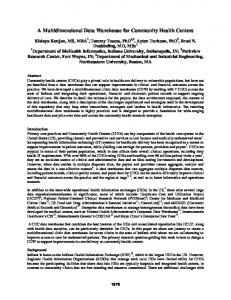
5.5.1

Equality Encoding on Generic Tags

In our first set of tests we computed the optimal number of bins for the worst case queries, i.e. queries with an attribute selectivity of 50%. All our calculations are based on the cost model presented in the previous sections. The total number of objects O is 106 and the size of the database page sp is 8 KB. In Figure 5.5 we plotted the I/O costs for handling queries over various dimensions and calculated the optimal number of bins for each of them. In addition, we also plotted the I/O costs for sequentially scanning the generic tags. As we can see, for one-dimensional queries the optimal number of bins is in the order of 1300. What is more, the resulting I/O costs are far below the sequential scan. For twodimensional queries, the optimal number of bins is in the order of 220 which is significantly less than for one-dimensional queries. However, the I/O costs are higher. For higher dimensional queries we can observe that the optimal number of bins gets even smaller. We can also see that for 15-dimensional queries the I/O costs for the optimal number of bins is slightly above the I/O costs for the sequential scan. For 25-dimensional queries the sequential scan always outperforms the bitmap index. In Figure 5.6 we plotted the same 50% attribute selectivity queries but we split the I/O costs for the bitmap index into following two additive phases, namely • index-I/O costs, i.e. costs for the Index Evaluation Phase • candidate-I/O, i.e. costs for the Candidate Check Phase We can see that the costs for index-I/O increase linearly with the number of bins (see Equation 5.5) whereas the costs for the candidate I/O decrease (see Equation 5.8). In our last calculations based on generic tags, we calculated the optimal number of bins for queries with lower attribute selectivities, namely 10%, 1% and 0.5%. (see Figure 5.7). Let us 53

4

page I/O − 2d

1

0 4 x 10

500

1000

1500

1.4 1.2 1 3

0 4 x 10

100

200

0

50

100 bins

150

200

300

1.6 0 4 x 10

50

100

150

200

200 bins

300

400

50% seq. scan 5

0

200

100

1.8

10

2

0 4 x 10

2

1.4

300

2.5

1.5

1

2.2

1.6

x 10

1.5

0.5

2000

page I/O − 10d

1.8 page I/O − 5d

2

1.5

0.5

page I/O − 15d

4

x 10

page I/O − 25d

page I/O − 1d

2

0

100

Figure 5.5: Generic tag - I/O costs for optimal number of bins for 50% attribute selectivity (worst case) compared to sequential scan.

start with analysing one-dimensional queries. For queries with an attribute selectivity of 10%, the optimal number of bins is in the order of 700. For attribute selectivities of 1% the optimum is in the order of 2000 bins whereas for queries 0.5% attribute selectivity the optimum is in to order of 3000 bins. We can observe the same behaviour for multi-dimensional queries. To sum up, for these low selectivities we can always find a optimal number of bins where the I/O costs are below the costs for the sequential scan. For higher selectivities the optimal number of bins is low, whereas for lower selectivities the optimal number of bins is high. The reason for this behaviour is that with high selectivities the index-I/O costs have a larger overhead than the resulting reduced overhead for the candidate I/O.

54

4

page I/O − 2d

2

1.5 1 0.5

2

0 4 x 10

500

1000

1500

3

0.5

page I/O − 15d

4

0 4 x 10

100

200

1 0

50

100 bins

150

200

300

0 4 x 10

50

100

150

200

200 bins

300

400

index−I/O cand−I/O 50% total 5

0

200

100

1

10

2

0 4 x 10

2

0

300

3

0

0.5 0

1

0

1

2000

1.5

x 10

1.5

page I/O − 10d

0

page I/O − 5d

4

x 10

page I/O − 25d

page I/O − 1d

2

0

100

Figure 5.6: Generic tag - I/O costs for optimal number of bins for 50% attribute selectivity (worst case) are split into index-I/O and candidate-I/O.

5.5.2

Equality Encoding on Sliced Tags

We will now look at the results for equality encoded bitmap indices based on sliced tags. Again we start with the analysis of the worst case for one-sided range queries, namely queries with attribute selectivities of 50%. In Figure 5.8 we can see a major difference to the worst case analysis for generic tags since for sliced tags, no typical optimum can be found. In particular, in all cases the I/O costs are increasing linearly with the number of bins and thus in all cases a low number of bins is desirable. What is more, the index is only more efficient than the sequential scan for queries over 10 dimensions and more. One of the main reasons for the good performance of the sequential scan is the advantage of the clustering for sliced tags. By looking at the separate cost components for the bitmap index, we can better interpret

55

4

page I/O − 2d

2

1.5 1 0.5

2

0 4 x 10

1000

2000

3000

3

0.5

page I/O − 15d

3

0 4 x 10

500

1000

1500

0

500

1000 bins

2000

3000

4000

0 4 x 10

500

1000

1500

2000

0.5% 1% 10% seq. scan

4 2 0

1500

1000

1

6

1

0 4 x 10

2

0

2000

2

0

0.5 0

1

0

1

4000

1.5

x 10

1.5

page I/O − 10d

0

page I/O − 5d

4

x 10

page I/O − 25d

page I/O − 1d

2

0

200

400

600

800

1000

bins

Figure 5.7: Generic tag - I/O costs for multiple attribute selectivities compared to sequential scan.

the results. In Figure 5.9 we see that the index-I/O again linearly increases with the number of bins. This is the same effect as for generic tags. However, since the candidate check is performed for each attribute separately, the costs for the candidate I/O (cand-I/O) are on average lower than the cand-I/O costs for generic tags. What is more, the cand-I/O decreases only marginally as the number of bins are increased. In our final analysis we evaluated the impact of queries with various selectivities. In short, we can again observe that for high selectivities a lower number of bins is better whereas for queries with low selectivities, a higher number of bins shows better I/O characteristics. One of the most important findings is that especially for high dimensional queries, the equality encoded bitmap index based on sliced tags has significantly lower I/O costs than the sequential scan.

56

6000 page I/O − 2d

page I/O − 1d

6000 4000 2000 0

0

100

200

300

400

4000 2000 0

500

2 page I/O − 10d

10000 5000 0

page I/O − 15d

3

0 4 x 10

100

200

300

1 0

0

50

100 bins

150

200

200

300

1 0.5 6

2

100

1.5

page I/O − 25d

page I/O − 5d

15000

0 4 x 10

0 4 x 10

50

100

150

200

100 bins

150

200

50% seq. scan 4 2 0

0

50

Figure 5.8: Sliced tag - I/O costs for optimal number of bins for 50% attribute selectivity (worst case) compared to sequential scan.

5.5.3

Comparison - Equality Encoding Generic Tags vs. Sliced Tags

When we compare equality encoded bitmap indices based on generic tags with indices based on sliced tags we can see that in most cases the total I/O costs are lower for bitmap indices based on sliced tags. We will thus base all our future analysis on sliced tags.

5.6

Partitioned Range Encoding

Since one-sided range queries (Q1r ) are the most common kind of queries in HEP, we also analysed range encoding [14] that performs considerably better than equality encoding. In contrast to [14] who based their optimisation techniques on discrete attribute values (where the problem of candidate and hit slices does not occur), we apply this method to contiguous values and thus a new optimisation method has to be considered. We refer to our approach as 57

6000 page I/O − 2d

page I/O − 1d

6000 4000 2000 0

0

100

200

300

400

4000 2000 0

500

2 page I/O − 10d

10000 5000 0

page I/O − 15d

3

0 4 x 10

100

200

0

0

50

100 bins

150

200

300

0.5 0 6

1

200

1

300

2

100

1.5

page I/O − 25d

page I/O − 5d

15000

0 4 x 10

0 4 x 10

50

100

150

200

100 bins

150

200

index−I/O cand−I/O 50% total

4 2 0

0

50

Figure 5.9: Sliced tag - I/O costs for optimal number of bins for 50% attribute selectivity (worst case) are split into index-I/O and candidate-I/O.

partitioned range encoding or in short range encoding. The main advantage over equality encoded bitmap indices is that in the worst case only one bit slice has to be scanned for one-sided range queries per dimension (independent of the selectivity of the query). As for equality encoded bitmaps, in the worst case half of the bit slices have to be scanned. Since we have already studied the behaviour of equality encoded bitmap indices and raised the I/O problem of candidate slices, we can easily conclude from these observations on the impact of range encoding. As already mentioned, in the worst case one bit slice needs to be scanned for one-sided range queries per dimension. This also implies that we have to consider only one candidate slice and no hit slice at all. Let us analyse the performance characteristics of one-sided range queries with both equality encoded and range encoded bitmap indices with variable selectivities, 10 6 objects and 10

58

1500 page I/O − 2d

page I/O − 1d

900 800 700 600 500

0

1000

2000

3000

5000

0

200

400

600

800

0

1000

2 page I/O − 25d

page I/O − 15d

1000

2000

3000

4000

5000

15000 10000 5000 0

0

10000 page I/O − 10d

page I/O − 5d

1000

500

4000

10000

0

0.5% 1% seq scan

0

100

200 bins

300

400

0 100 4 x 10

200

300

400

500

0.5% 1% 10% seq. scan

1.5 1 0.5 0

0

100

200 bins

300

400

Figure 5.10: Sliced tag - I/O costs for multiple attribute selectivities compared to sequential scan.

indexed attributes. Again we studied the performance characteristics of the bitmap index on uniformly distributed data. As we can see in Figure 5.11, the query time for equality encoded bitmap indices increases with increasing selectivities (i.e. a higher number of hit slices has to be read) whereas the query time for range encoded bitmap indices is more or less constant for all selectivities (since no hit slices at all have to be scanned). The fact that only one bit slice needs to be scanned gives us much more freedom in extending the number of bins until the theoretical maximum of the cardinality of the attribute value. Since we are dealing with contiguous values, we do not have a finite cardinality and hence are mainly “restricted” by the space complexity. We thus end up in a “practical” optimisation problem, that is constraint by the available disk space. Experimentally we can show that the behaviour of a range encoded bitmap index both for Q1r and Q2r corresponds to a partial scan over the event data. The performance character59

25

20

Time [sec]

15

10 EQ Range

5

0

0

10

20

30

40

50 Selectivity

60

70

80

90

100

Figure 5.11: Partitioned Equality Encoding (EQ) vs. Partitioned Range Encoding (Range). istics are thus highly dependent on the characteristics of the underlying OODBMS, namely Objectivity/DB and the disk. In particular, for page selectivities between 5% and 100%, the read rate is almost linear. However, a significant speedup is achieved, if the page selectivity is smaller than 5% [33] which in turn is very common for multi-dimensional range queries in HEP analysis. A detailed analysis on range encoded bitmap indices is given in the next chapter.

5.7

Conclusions

We have given analytical performance studies of bitmap indices for scientific data and pointed out the main difference to other studies on bitmap indices - those that concentrated on only discrete attribute values. The main bottleneck has been shown to be the checking of the candidate slices due to the additional I/O for fetching the event data from disk in addition to the I/O for the bitmap index. We have designed and implemented our bitmap indices on top of a commercial object database management system, namely Objectivity/DB and used different bitmap encoding techniques for our analysis. We presented a novel cost model for evaluating equality encoded bitmap indices and showed analytically the optimal number of bins for various multidimensional range queries with different query selectivities. This optimum can be regarded as a trade-off between a high number of candidates and consequently more I/O on the event data vs. a low number of candidates and therefore a higher number of bins. Since HEP queries are mainly one-sided range queries, we also studied partitioned range encoding. We showed that the performance of range encoded bitmap indices clearly outperforms equality encoded bitmap indices.

60

Chapter 6

Generic Range Encoding 6.1

Introduction

In the previous chapter we discussed equality encoded bitmap indices and introduced a cost model for calculating the optimal number of bins for various queries. We also gave a brief outlook to range encoded bitmap indices. The advantage of this encoding technique is that in the worst case only one bit slice needs to be scanned for evaluating one-sided range queries. As for equality encoded bitmap indices in the worst, half of the bit slices need to be scanned Chan and Ioannidis [14] introduced an index evaluation algorithm based on range encoding which guarantees that only one bit slice needs to be scanned for evaluating one-sided range queries. However, the algorithm is designed for discrete attribute values but does not take into account non-discrete attribute values such as floating point values which are very typical for scientific data. In this chapter, we present a novel algorithm for processing both one-sided and twosided range queries via bitmap indices over floating point values. Our algorithm is called GenericRangeEval since it is a generalisation of the other algorithms [14] for one-sided range queries and supports efficient query processing for scientific data. We also extend the cost model introduced in the previous chapter for predicting the performance of range encoded bitmap indices based on uniformly distributed and independent data values. We evaluate the minimal required index size for querying high-dimensional search spaces and discuss the trade-off between index size and performance. Besides a detailed description of our analytical model we also give a performance study and show up to which dimensionality and query selectivity the bitmap index performs better than sequentially scanning the base objects.

6.2

Example: Range Encoding for Non-Discrete Attribute Values

As we mentioned already previously, the range-encoding technique introduced by [14] is only optimised for discrete attribute values. The main difference of indexing non-discrete data is that not the attribute cardinalities can be encoded but attribute ranges. For instance, 61

[0;120) [0;100) [0;80) [0;60) [0;40) [0;20)

34.7

1

1

1

1

1

0

94

1

1

0

0

0

0

64.9

1

1

1

0

0

0

15.5

1

1

1

1

1

1

61.7

1

1

1

0

0

0

137.2

0

0

0

0

0

0

8.6

1

1

1

1

1

1

bin ranges candidate object (no hit)

candidate object (is "hit")

query range: x 63 rather than x < 63 as previously. The query mapping step (line 1.3) again yields slice 3 but due to the “greater operator” in the query predicate, the temporary bit slice T is now T = B2 (see lines 1.6 and 1.22). However, B2 represents all objects with values less than 60. By negating this bit slice (line 1.11) we obtain all objects with values greater or equal 60, i.e. range [60;140). We call this bit slice again “candhits” (line 1.27 CHd = T ). The “candidate mask” is similar to the previous example. After increasing the current bit slice by one (see line 1.29), the actual candidate objects without including the hit objects are yielded by Cd = B3 XOR B2 (lines 1.36 and 1.31). It is important to note that additional “operator checks” need to be included into the algorithm which guarantee that the query range is mapped correctly to the corresponding bit slice and is then also evaluated correctly. Just to give one example of this additional complexity, assume that instead of x > 63 our query is x ≤ 60. In that case, bit slice B2 contains (with

64

attribute 1

attribute 2

attribute 3

1

1

1

1

0

1

1

1

1

0

1

1

1

1

0

1

0

0

0

0

1

0

0

0

0

1

0

0

0

0

1

1

0

0

0

1

1

0

0

0

1

1

0

0

0

1

1

1

1

1

1

1

1

1

1

1

1

1

1

1

1

1

0

0

0

1

1

0

0

0

1

1

0

0

0

0

0

0

0

0

0

0

0

0

0

0

0

0

0

0

1

1

1

1

1

1

1

1

1

1

1

1

1

1

1

XOR

XOR

XOR

"candidate check"

AND AND

candidate check on reduced number of candidates

candidate check on reduced number of candidates

Figure 6.2: Candidate check in multi-dimensional space. For each attribute the candidates are checked separately.

certainty) only hits whereas bit slice B3 is our “candhits” slice CHd where we would need to filter out the hit objects. The behaviour of the bitmap index in the multi-dimensional space is depicted in Figure 6.2. Note that for each attribute the candidate check is done separately, e.g after “XOR”ing the “candhits” slice with the “previous” slice as shown for the query x < 63. However, for all remaining attributes, the bit slice which is yielded after “XOR”ing, is “AND”ed together with the “global” hit slice H (see line 1.14). This means, for example, that for attribute 2 only these candidate objects need to be checked against the query constraint that are hits of attribute 1. The resulting positive effect of this approach is that with a low “attribute query selectivity” the number of candidate objects for each further dimension gets reduced. Finally, the hits of each dimension are “AND”ed together (line 1.16). The whole algorithm for evaluating one-sided range queries based on range-encoded bitmap indices is shown below. Note that for simplicity we assume that all attributes are global so that parameters do not need to be passed explicitly when a function is called. Algorithm: GenericRangeEval for one-sided range queries 1.01) for d=0 to D-1 65

1.02)

evaluate query()

Function: evaluate query() 1.03) s = qd mapped to the bit slice 1.04) s0 = s; cand mask=false; 1.05) if opd ∈ {>, ≥} OR (opd ∈ { 0 ) then Cd = Cd AND H candidate check() H = H AND CHd

Function: evaluate cands() 1.17) if (s < nd ) then 1.18) if opd ∈ {>, ≥} AND s0 == 0 then 1.19) T =set all bits to 0 1.20) Cd =B0 1.21) cand mask=true 1.22) else T =Bd,s 1.23) else 1.24) T =set all bits to 1 1.25) Cd =NOT Bd,nd−1 1.26) cand mask=true Function: merge candhits() 1.27) CHd = T Function: mask cands() 1.28) if opd {=} then 1.29) if opd ∈ {>, ≥} AND s0 0 then s=s+1 1.30) evaluate equality(T1 ) 1.31) Cd =T1 1.32) else Cd =T 1.33) cand mask=true Function: evaluate equality(Tret ) 1.34) if (s==0) then return Tret =Bd,s 66

1.35) 1.36)

else if (s==nd) then return Tret =NOT Bd,s−1 else return Tret =Bd,s XOR Bd,s−1

Function: candidate check() 1.37) check Cd against query constraint 1.38) if candidate is no hit then turn off bit in CHd The algorithm described above handles the case of one-sided range queries. For the slightly more complex case of two-sided range queries, a few changes need to be made in three functions. In short, the main function evaluate query needs to be called twice, namely the first time for the “lower range” (line 2.04) and the second time for the “upper range” (lines 2.05 - 2.07) of the query predicate. When then “upper range” is evaluated, the “candhits” of the particular dimension must be “AND”ed together (line 2.20), whereas the “cands” must be “OR”ed together (lines 2.07, 2.15, 2.27 and 2.32). Algorithm: GenericRangeEval for two-sided range queries Function: evaluate cands() 2.01) if (s < nd ) then 2.02) if opd ∈ {>, ≥} AND s0 == 0 then 2.03) T =set all bits to 0 2.04) if (lower range) then Tc = B0 2.05) else 2.06) Cd = B0 2.07) Cd = Cd OR Tc 2.08) cand mask=true 2.09) else T =Bd,s 2.10) else 2.11) T =set all bits to 1 2.12) if (lower range) then Tc = NOT Bd,nd−1 2.13) else 2.14) Cd = NOT Bd,nd−1 2.15) Cd = Cd OR Tc 2.16) cand mask=true Function: merge candhits() 2.17) if (lower range)then Tch = T 2.18) else 2.19) CHd = T 2.20) CHd = CHd AND Tch Function: mask cands() 2.21) if opd {=} then 2.22) if opd ∈ {>, ≥} AND s0 0 then s=s+1 2.23) evaluate equality(T1 ) 67

2.24) 2.25) 2.26) 2.27) 2.28) 2.29) 2.31) 2.32) 2.33)

if (lower range)then Tc = T1 else Cd = T1 Cd = Cd OR Tc else if (lower range)then Tc = T 2.30) Cd = T Cd = Cd OR Tc cand mask=true

6.4

Cost Model for GenericRangeEncoded Bitmap Indices

else

In the previous chapter we discussed the optimal number of bins for equality encoded bitmap indices and introduced a cost model for studying analytically the I/O complexity of the bitmap index. We will now extend this cost model for range encoded bitmap indices based on the novel algorithm called GenericRangeEval.

6.4.1

I/O Complexity of the Index

In order to evaluate the I/O complexity of the bitmap index including the overhead for the candidate check, we separate the algorithm GenericRangeEval into two phases, namely • Index Evaluation Phase • Candidate Check Phase Let us first start with the Index Evaluation Phase, i.e. the number of I/O operations needed for scanning the bitmap index in order to evaluate a query. The Index Evaluation Phase does not include the I/O operations for the candidate check. According to [14] only one full bit slice scan is needed for evaluating a one-sided range query with a conventional range-encoded bitmap index. However, GenericRangeEval requires slightly more bit slice scans due to the masking of candidate objects. In particular, one bit slice scan is needed for identifying the “candhits” slice (see line 1.22). In addition, one or two bit slice scans are required for filtering out (masking) the candidates from the “candhits” slice (lines 1.34 - 1.36). To sum up, three bitmaps scans are required for a one-dimensional one-sided range query. Informally for a d-dimensional query, the following number of bit slice scans b are required in the worst case: b = 3 · bitmap · d

(6.2)

where bitmap refers to a full bitmap scan and d to the number of dimensions covered by the query. We will interpret bitmap in terms of page-I/Os in the next sub-section.

68

Parameter Description O Ec d bi sp pi ps

total number of objects expected number of candidate objects which need to be checked against query constraint number of dimensions number of bit slices of dimension i page size (in bytes) total number of pages for storing all objects of dimension i number of pages for storing one bit slice Table 6.2: Parameters of the cost model.

After the index evaluation phase, the candidate objects are checked against the query constraint. The number of candidates depends on the query selectivity and the number of bins (bit slices).

6.4.2

Page I/O Costs for Index Evaluation Phase

Similar to the previous chapter, for the Index Evaluation Phase we need to express the number of bitmaps to be accessed in terms of database pages. In addition, the number of pages for reading the expected number of candidates during the Candidate Check Phase needs to be calculated. By adding the number of page I/Os for these two phases, the costs of accessing the data objects via the bitmap index can be compared to the costs of accessing the data directly without the index. The parameters of our model are described in Table 6.4.2. If we substitute bitmap in Equation 6.2 with ps , the I/O costs in terms of database pages for the index evaluation phase Ci can simply be computed as: Ci = 3ps d

(6.3)

where ps is the number of database pages for storing one bit slice and is given as: ps =

O 8sp

(6.4)

Note that we divide O by 8 in order to reflect the size of a bit slice in bytes.

6.4.3

Page I/O-Costs for Candidate Check Phase

Basically, the main bottleneck of bitmap indices on non-discrete attribute values is the additional disk I/O overhead for checking the candidate objects against the query constraint. A straightforward approach to relax this bottleneck is to increase the number of bins and thus the number of candidate objects in each bin. The main question to be answered is what is the minimal index size needed and which index size is “practically feasible”. The equation for

69

#bins index size [bytes] #cand. objects #pages to read page selectivity 10 50 100 200 500 1’000 1’500 2’000 4’000

1’179’648 6’422’528 12’976’128 26’083’328 65’404’928 130’940’928 196’476’928 262’012’928 524’156’928

100’000.00 20’000.00 10’000.00 5’000.00 2’000.00 1’000.00 666.67 500 250

620 620 620 620 596 497 409 344 206

1 1 1 1 0.960276 0.800692 0.658794 0.553561 0.331839

Table 6.3: Effect of number of bins on the number of candidate objects for one dimension.

calculating the I/O overhead for the Candidate Check Phase corresponds to Equations 5.10 and 5.11 for sliced tags of the previous chapter. For ease of understanding, we will repeat them here again: c −E p

Ccsliced = pi (1 − e

i

)

(6.5)

and Ecsliced =

d O O X + seli−1 b1 i=2 bi

(6.6)

For all our tests assume 106 objects and a database page size sp of 8KB. Thus, the base objects for one dimension comprises 620 pages, in our example with 100 bins we need to read 620 pages for the candidate check. In other words, with this low number of bins, the bitmap index does not yield any improvement over sequentially scanning over the base objects without using an index. In Table 6.4.3 we show the effect of various numbers of bins on the number of pages to be read (page selectivity) during the candidate check. As we can see, with 1000 bins only 497 pages need to be read which corresponds to a page selectivity of 80%. With 2000 bins the page selectivity drops to 55%. However, the main disadvantage is certainly the size of the index. For example, with 1000 bins the size of the index is about 25 times the size of the base objects. In short, we can conclude that this kind of index is not very “practical” for one-dimensional queries, however, the bitmap index shows its strength in high-dimensional space with queries of relatively low selectivities (see Figure 6.2). We will go into further detail in the next section. The total costs Ctot for evaluating one-sided range queries in terms of page I/Os is the sum of the I/O-costs for the Index Evaluation Phase Ci (see Equation 6.3) and the Candidate Check Phase Cc (see Equations 6.5 and 6.6) :

70

Ctot = 3ps d +

d X

−

pi (1 − e

Eci pi

)

(6.7)

i=1

where ps is defined according to Equation 6.4. Eci is defined according to Equation 6.5.

6.5

Analytical Results

On presenting a cost model for predicting the I/O complexity of the bitmap index, we will now evaluate analytically the performance of the bitmap index for multi-dimensional queries. During our tests we carried out one-sided range queries over various dimensions starting from 1 to 25. For each dimension we varied the selectivity from 10% up to 100%. Similar to the previous chapter, the selectivity of the queries is depicted as the selectivity per dimension. For example, in the case of 5 dimensions the query selectivities for each dimension range from 0.1 to 1.0. If we calculate the corresponding total selectivity for uniformly distributed and independent data values then it ranges from 0.15 (0.00001) to 1.05 (1.0). In particular, we are interested in studying following additive phases for evaluating a query via bitmap indices: • Index-I/O: Overhead for scanning the bit slices of the index. • Candidate-I/O: Index-I/O including the I/O operations for checking the candidate objects against the query constraint. • Hit-I/O 1: Candidate I/O including the I/O operations for retrieving the hits. • Hit-I/O 2: Candidate I/O including the I/O operations for retrieving the hits of only one attribute. We also varied the number of bins from 10 to 1000 to study the effect on the candidate I/O. Finally, we plotted the results for the theoretical maximum of 1,000,000 bins, i.e. for each attribute value one bin. In Figure 6.3 we plotted the page I/O costs for queries over multiple dimensions against the bitmap index with 10 bins per indexed attribute. For each dimension we can observe a constant index-I/O overhead independent of the query selectivity. As we can see in the cost model (see Equation 6.7), for each dimension at most 3 bit slices need to be scanned in order to evaluate any kind of one-sided range query. The page I/O costs for the candidate I/O are always higher than the costs for the sequential scan up to three-dimensional queries (see Figure 6.3). For five-dimensional queries, the candidate I/O is below the sequential scan up to an attribute selectivity of 20%. For ten and 25 dimensions, the candidate I/O overhead is below the sequential scan up to 60% and 80% attribute selectivity respectively. In short, due to the low number of bins, the candidate I/O overhead gets only outweighed for high-dimensional queries. We also studied the impact on the costs for retrieving the hits. hit I/O 1 shows the I/O costs for retrieving the hits of each indexed attribute after all candidate objects for each attribute are evaluated. 71

3000 page I/O − 2d

page I/O − 1d

1500 1000 500 0

0

20

40

60

80

0

3000 2000 1000

40

60

80

100

0

20

40

60

80

0 20 4 x 10

40

60

80

100

20 40 60 80 selectivity per dimension

100

4000 2000 0

100

4 page I/O − 25d

page I/O − 10d

20

6000

15000 10000 5000 0

0

8000 page I/O − 5d

page I/O − 3d

1000

100

4000

0

2000

0

20 40 60 80 selectivity per dimension

100

3 2

index I/O incl. cand I/O incl. hit I/O 1 incl. hit I/O 2 seq. scan

1 0

0

Figure 6.3: Analytical results: Page I/O for queries over multiple dimensions with various selectivities. 10 bins.

In High Energy Physics it is very common to perform multi-dimensional queries but later on only plot the results of one attribute in a histogram. Thus, we also evaluated these hit I/O costs. Throughout the analytical results these I/O costs are referred to hit I/O 2. In Figure 6.4 we carried out the same set of queries on a bitmap index with 100 bins per indexed attribute. The main effect of the increased number of bins is a reduced candidate I/O overhead since each bin contains fewer candidate objects than with 10 bins (as we have seen in the previous figure). Thus, the pay-off for the index can already be seen for lower dimensional queries with higher attribute selectivities. In particular, the candidate I/O is below the sequential scan for three-dimensional queries up to 20% attribute selectivity. For five-dimensional queries the threshold moves up to 50% attribute selectivity, for ten dimensions up to 80% and for 25 dimensions up to 90%. Considering also the hit I/O in Figure 6.4, the bitmap index is more I/O efficient than the sequential scan starting from five dimensions up to attribute selectivities of 20% for hit I/O 1 72

3000 page I/O − 2d

page I/O − 1d

1400 1200 1000 800 600

0

20

40

60

80

1500

3000 2000

40

60

80

100

0

20

40

60

80

0 20 4 x 10

40

60

80

100

20 40 60 80 selectivity per dimension

100

4000 2000 0

100

4 page I/O − 25d

page I/O − 10d

20

6000

15000 10000 5000 0

0

8000 page I/O − 5d

page I/O − 3d

2000

1000

100

4000

1000

2500

0

20 40 60 80 selectivity per dimension

100

incl. cand I/O incl. hit I/O 1 incl. hit I/O 2 seq. scan

3 2 1 0

0

Figure 6.4: Analytical results: Page I/O for queries over multiple dimensions with various selectivities. 100 bins.

and up to 30% for hit I/O 2. For ten and 25-dimensional queries, the bitmap index becomes even more efficient. In the following two figures (6.5 and 6.6) we show that by increasing the number of bins, the candidate I/O overhead can even be more decreased and thus the bitmap index shows even better performance characteristics. This is especially true for lower dimensional queries. Figure 6.6 shows the I/O overhead for queries against a bitmap index with 1,000,000 bins per indexed attribute. This index size is the theoretical upper limit for 1,000,000 base objects. Since each object is represented by a bit slice, the overhead for the candidate I/O converges to zero and thus only the constant overhead for the index I/O is left. We have thus demonstrated that the I/O overhead for the bitmap index based on discrete attribute values can be reduced by increasing the number of bins and thus the size of the index. However, reduced bitmap index overhead results in additional storage overhead.

73

2500 page I/O − 2d

page I/O − 1d

1200 1000 800 600 400

0

20

40

60

80

1000

3000 2000 1000

40

60

80

100

0

20

40

60

80

80

100

20 40 60 80 selectivity per dimension

100

2000 0

100

3 page I/O − 25d

page I/O − 10d

20

4000

15000 10000 5000 0

0

6000 page I/O − 5d

page I/O − 3d

1500

500

100

4000

0

2000

0

20 40 60 80 selectivity per dimension

100

0 20 4 x 10

2

40 60 incl. cand I/O incl. hit I/O 1 incl. hit I/O 2 seq. scan

1 0

0

Figure 6.5: Analytical results: Page I/O for queries over multiple dimensions with various selectivities. 1,000 bins.

6.6

Experimental Results

In this section we evaluate the performance of the bitmap index experimentally and compare the results to our analytical study. One of the main questions which we will answer throughout the experiments is to find out up to which dimensionality under a given query selectivity the presented index data structure performs better than the sequential scan. We carried out all our experiments on a Pentium II 400 under Linux Red Hat 6.1. The multi-dimensional bitmap index is implemented on top of Objectivity/DB version 5.1.2. All experiments operate on 106 objects with 1 to 25 attributes (dimensions) with uniformly distributed and independent data values. Table 6.6 shows the size of these objects and the query response time for sequentially reading them. Similar to the previous section on analytical results, we carried out one-sided range queries over various dimensions starting from 1 to 25. The size of the index is 100 bins per attribute 74

1500 page I/O − 2d

page I/O − 1d

800 600 400 200 0

0

20

40

60

80

0

2000 1000

40

60

80

100

0

20

40

60

80

0 20 4 x 10

40

60

80

100

20 40 60 80 selectivity per dimension

100

2000 1000 0

100

2 page I/O − 25d

page I/O − 10d

20

3000

8000 6000 4000 2000 0

0

4000 page I/O − 5d

page I/O − 3d

500

100

3000

0

1000

0

20 40 60 80 selectivity per dimension

1.5 1 0.5 0

100

incl. cand I/O incl. hit I/O 1 incl. hit I/O 2 seq. scan

0

Figure 6.6: Analytical results: Page I/O for queries over multiple dimensions with various selectivities. 1,000,000 bins.

resulting in a total bitmap index size which is in the order of three larger than the base objects. For each dimension we varied the selectivity from 10% up to 100% in order to study the following phases: • Index-I/O: Overhead for scanning the bit slices of the index. • Candidate-I/O: Index-I/O including the I/O operations for checking the candidate objects against the query constraint. • Hit-I/O 1 (non-interleaved): Candidate I/O including the I/O operations for retrieving the hits. • Hit-I/O 2 (interleaved): Candidate I/O including the I/O operations for retrieving the hits. In this case, the hits are retrieved in smaller “segments” and thus the result of the first set of objects can be retrieved earlier. 75

Dimensions data size [MB] response time 1 2 5 10 15 25

4.9 9.7 24.5 52.7 80.1 137.1

8.7 11.4 22.9 42.5 62.4 103.3

Table 6.4: Response time for sequential scan over 106 objects with various number of attributes (dimensions) - attribute-wise clustering.

• Seq. scan: Comparison of the bitmap index with sequentially scanning the base objects. Let us first analyse the case of a one-dimensional query against the bitmap index with 100 bins and compare it to the sequential scan which takes 8.7 seconds and requires 602 page I/Os (see Figure 6.7). The overhead for scanning the bit slices of the one-dimensional index is constant and requires 112 page I/Os or 1.3 seconds (index-I/O). Note that for the case of 100% selectivity both the page I/O and the response time go slightly down. This is because the last bin requires fewer bit slice operations for evaluating the query. Next we plotted the candidate I/O which corresponds to the index-I/O and the additional I/O operations for checking the candidate objects against the query constraint. The costs for the page I/O are about 10% more than the costs for the sequential scan (sequential case). This is because with 100 bins the page selectivity for the candidate check is 100% which means that all attribute values must be fetched from disk in addition to the index-I/O. Consequently, also the response time for the query via the index is slightly higher than the sequential case. The next two plots include the I/O-operations for fetching the hits from disk. In the case hit-I/O 1 all objects are evaluated and then the hits are fetched from disk. As for hit-I/O 2 a subset of the objects is evaluated and fetched from disk interleaved. In particular, the first 10,000 objects are evaluated and then the hits are fetched from disk. Afterwards, the next 10,000 objects are evaluated and then fetched from disk, etc. The advantage of hit-I/O 2 is that fewer number of pages need to be read. For two-dimensional queries (see Figure 6.7) all page I/O operations are above the sequential case. However, hit-I/O 2 is more efficient than the sequential case up to an attribute selectivity of 40%, which corresponds to a total query selectivity of 16%. Three-dimensional queries are more efficient than the sequential case up to an attribute selectivity of some 60% (total selectivity 21%). Note that the difference between hit-I/O 1 and hit-I/O 2 gets smaller since the total number of hits is reduced and thus the positive effect of interleaved hit I/O is less significant. Starting from five-dimensional queries (see Figure 6.8) we can observe a further effect in the slope of the query response time, namely a “flat segment” of the curve for hit-I/O 1 and hit-I/O 2 for attribute selectivities between 20% and 50%. This is due to the overhead of the disk head movements for random access. In short, even though the page I/O decreases as the 76

15 time [sec] − 1d

page I/O − 1d

1500 1000 500 0

0

20

40

60

80

time [sec] − 2d

page I/O − 2d

2000 1000 0

20

40

60

80

20

40

60

80

100

60

80

100

20 40 60 80 selectivity per dimension

100

20 10 0

100

0

30 time [sec] − 3d

4000 page I/O − 3d

0

30

3000

3000 2000 1000 0

5 0

100

4000

0

10

0

20 40 60 80 selectivity per dimension

20 10 0

100

20 40 index I/O incl. cand I/O incl. hit I/O 1 incl. hit I/O 2 seq. scan

0

Figure 6.7: Experimental results: Page I/O and response for queries over multiple dimensions with various selectivities - one to three dimensions.

query selectivity decreases, the advantage of random access vs. sequential access does not pay off for any random access pattern. With 25-dimensional queries the bitmap index including hit-I/O is more efficient than the sequential case up an attribute selectivity of 90% (total selectivity 0.925 ). It is important to note that for low selectivities, the response time of the hit-I/O is about twice as much as the response time for the index-I/O. For high selectivities, in particular for an attribute selectivity of 90%, the ratio increases up to a factor of 8.

6.7

Analytical vs. Experimental Results

The experimental results in Figures 6.7 and 6.8 show that the cost model can predict the I/O complexity for the bitmap index with an error of 10% to 20% for 25-dimensional queries. In

77

60 time [sec] − 5d

page I/O − 5d

8000 6000 4000 2000 0

0

20

40

60

80

page I/O − 25d

time [sec] − 10d 0 20 4 x 10

40

60

80

20

40

60

80

100

0

20

40

60

80

100

2 1 20 40 60 80 selectivity per dimension

20 40 60 80 selectivity per dimension

100

index I/O incl. cand I/O incl. hit I/O 1 incl. hit I/O 2 seq. scan

300

3

0

50

0

100

time [sec] − 25d

page I/O − 10d

5000

0

0

100

10000

4

20 0

100

15000

0

40

100

200 100 0

0

Figure 6.8: Experimental results: Page I/O and response for queries over multiple dimensions with various selectivities - five to 25 dimensions.

78

particular, the cost model sytematically underestimates the real costs between 10% to 20%. However, this accuracy is good enough for a query optimiser to decide between two access methods, namely whether to access all the data sequentially without using an index or to use the index.

6.8

Conclusions

We presented a novel algorithm for evaluating range queries called GenericRangeEval and studied analytically and experimentally the performance behaviour of multi-dimensional queries with various query selectivities. Initially the algorithm was designed to evaluate typical onesided range queries but by a simple extension, the algorithm can also efficiently handle the more general case of two-sided range queries. One of the most crucial design parameters is the number of bins of the index. In short, a larger number of bins results in a lower number of candidate objects which need to be checked against the query constraint. In other words, the larger the number of bins, the lower the response time of the bitmap index. On the other hand, a larger number of bins also increases the size of the bitmap index significantly. Thus, the choice of the number of bins is always a trade-off between speed and space. Experimentally we evaluated the results yielded from the analytical cost model. We demonstrated that the cost model gives a fairly accurate estimation about the I/O complexity of the bitmap index. Thus, by calculating the I/O costs of the bitmap index prior to query execution, a query optimiser can easily decide whether to handle the query via the bitmap index or whether it is more efficient to sequentially scan over the base objects without using an index at all. We based our experimental results on an index with 100 bins which is about three times the size of the base objects. We showed that for low dimensional queries the candidate check overhead of the bitmap index is the main bottleneck and thus the sequential scan is often faster. However, for high dimensional queries with low attribute selectivities (which is the main use case for HEP) the bitmap index shows a significant performance improvement over the sequential scan up to a factor of 5 for a 25-dimensional search space.

79

Chapter 7

Advanced Features 7.1

Introduction

In the previous chapters we analysed the impact of different kinds of bitmap encoding techniques on the query response time. We concluded that equality encoding is optimised for exact match queries whereas range encoding is optimised for range queries. In this chapter we will discuss further optimisation techniques for tuning the performance of the bitmap index, such as an adaptive index, different binning strategies and bitmap compression. In particular, we will analyse the impact of bitmap compression on uniformly and non-uniformly distributed data.

7.2

Adaptive Index

One of the simplest and most efficient adaptive techniques of the index based on GenericRangeEncoding is to evaluate first the attribute (dimension) which has the lowest attribute selectivity. The advantage of this approach is that the search space gets pruned already very early so that the result set for the evaluation of higher dimensions is reduced. Consider this simple 3-dimensional query based on a search space in the range of [0;100] with uniformly distributed data values. A possible query execution plan is as follows: a0 < 40 AND a1 > 95 AND a2 < 47 The attribute selectivity of a0 is 40%, of a1 5% and of a2 47%. Thus, the query can be more efficiently evaluated by ordering the attributes (dimension) according to increasing attribute selectivities. Assuming left-to-right evaluation, the optimal query execution plan is as follows: a1 > 95 AND a0 < 40 AND a2 < 47

80

7.3

Binning Strategies

A further important turning parameter of the bitmap index is the binning. Up to now, we only assumed so-called equi-width bins, which means that each bin has the same width and thus the distribution of the data values is also reflected in the number of entries for each bin. In Chapter 5 we briefly discussed this kind of binning strategy. Besides equi-width binning, there is also the possibility of equi-depth binning which guarantees that each bin has the same number of entries. Both binning strategies have advantages and disadvantages which we will discuss in this section. In short, the binning strategy depends on two factors, namely the data distribution and the query access patterns (or the query distribution). Equi-depth binning guarantees nearly constant access time for all kind of queries independent of the data distribution. One would chose this kind of binning when no query access patterns are available. Since equi-width bins reflect the data distribution, this kind of binning is preferable if the query access patterns are such that those bins are queried most, which have the least number of entries. If the query access patterns are well understood, the binning could be even more adapted. Thus, for heavily queried regions in the search space, the bin ranges should be narrow such that these bins only have a small number of entries. On possible solution to this problem is given in [40].

7.4

Bitmap Compression on Uniformly Distributed Data

In Chapter 6 we discussed the typical space/time trade-off when designing a bitmap index. In short, the larger the number of bins, the lower the query response time of the bitmap index. On the other hand, a larger number of bins also increases the size of the bitmap index significantly. One way to reduce the space complexity is to compress the index. However, the requirement for a good bitmap compression algorithm is not only to have a good compression ratio but also to show good performance during the logical operations between the bit slices. In the following sub sections we discuss the impact of compression on equality encoded and range encoded bitmap indices. According to [15] equality-encoding shows good compressibility due to the sparse bit slices whereas range-encoding shows better performance on a verbatim bitmap index. We will extend this study and compare the relative performance for all combinations thereof, i.e. equality encoding vs. range encoding on compressed and verbatim bitmap indices, in order to classify the best encoding technique for different kinds of query types. Together with Theodore Johnson from AT&T Labs-Research we implemented a slightly improved version of the original Byte-Aligned Bitmap Compression [39] algorithm by [1]. The algorithm is briefly described in Chapter 3.

7.4.1

Equality Encoded Bitmap Index

We again base our experiments on 1,000,000 objects with uniformly distributed data values. First we compare the size of a bitmap index of 100 bins for verbatim bit slices and for compressed ones. The size of the verbatim bitmap index for one attribute is some 13.5 MB whereas 81

the size of the compressed bitmap index is some 2 MB. The compression factor of each bit slice is roughly 9. However, the compression factor of the whole bitmap index is only around 7 due to some constant overhead of an Objectivity database (which is about 0.5 MB). For 1000 bins the size of the verbatim bitmap index is 140 MB and of the compressed index 8.5 MB. This corresponds to a compression factor of 16.5 for the whole bitmap index. For the following tests, we studied the I/O costs and the response time of a 1-dimensional query based on a compressed equality encoded bitmap with 100 and 1000 bins. Since we want to evaluate the compression algorithm, we only report on the results of evaluating the query via the bitmap index and ignore the candidate I/O at this stage. With 100 bins, the query response time of the compressed bitmap is lower than the verbatim bitmaps for an attribute selectivity above 20% (see Figure 7.1). Even though the number of page I/Os is always lower than for the verbatim case, there is additional CPU overhead of the compressed index which results in a worse performance for queries with selectivities below 20%. 900

5 verbatim compressed

800

4.5

700 4

time [sec]

page I/O

600

500

3.5

3 400 2.5 300

2

200

100 10

20

30 selectivity

40

1.5 10

50

20

30 selectivity

40

50

Figure 7.1: Query response time of verbatim vs. compressed equality encoded bitmap index 100 bins. With 1000 bins the advantage of the compressed bitmap index over the verbatim one becomes very significant (see Figure 7.2). For a query selectivity of 10% the query response time of the compressed bitmap index is a factor of two lower than for the verbatim one. For a query selectivity of 50% the compressed bitmap index is even a factor of 3 faster than the

82

verbatim one. 9000

40 verbatim compressed

8000

35

7000 30 6000

5000

time [sec]

page I/O

25

4000

20

15 3000 10 2000 5

1000

0 10

20

30 selectivity

40

0 10

50

20

30 selectivity

40

50

Figure 7.2: Query response time of verbatim vs. compressed equality encoded bitmap index 1000 bins.

These results clearly demonstrate the advantage of compressed over verbatim equality encoded bitmap indices.

7.4.2

Range Encoded Bitmap Index

As already pointed out by [15] the compression ratio for range encoded bitmap indices is relatively poor in comparison to the sparser representation of equality encoded bitmaps. We evaluated the compression ratio for a bitmap index of 100 bins on 1,000,000 objects with uniformly distributed data values. In Figure 7.3 we plotted the compression ratio of each single bin of the bitmap index. As we can see, the compression ratio is only below 0.5 for 7% of the bins. All remaining bins are hardly compressible (until about 15% of the bins) or not compressible any more - the latter is true for 85% of the bins. For 1,000 bins the compression ratio shows a similar pattern. To sum up, bitmap compression for range encoded bitmap indices with uniformly distributed attribute values is practically not feasible.

83

1.1

1

0.9

Compression ratio

0.8

0.7

0.6

0.5

0.4

0.3

0.2

0.1

0

10

20

30

40

50 bin

60

70

80

90

100

Figure 7.3: Compression ratio of range encoded bitmap index with 100 bins.

7.4.3

Compressed Equality Encoding vs. Verbatim Range Encoding

As we have demonstrated in the previous sections, equality encoded bitmap indices show good compressibility and also a better performance than verbatim equality encoded bitmap indices. As for range encoding, verbatim bitmap indices show better performance characteristics due to the relatively poor compressibility of the bitmaps. Thus, in this section we compare the two “winners” of our evaluation, namely compressed equality encoded vs. verbatim range encoded bitmap indices and show up to which selectivity one technique shows better performance than the other one. Let us now evaluate the impact of bitmap compression for multi-dimensional queries. We assume an equality encoded bitmap index with 1000 compressed bit slices and compare it to a range encoded bitmap index with 100 bins. Due to the good compressibility of the equality encoded index, the size of the compressed bitmap index with 1000 bins is about 60% of the size of the uncompressed bitmap index with 100 bins. Our main focus of interest is a direct comparison of the compressed equality encoded bitmap index with a verbatim range encoded one. We thus perform similar benchmarks as depicted in Figures 6.7 and 6.8 of the previous chapter. In particular, we will study the number of page I/Os and the response time for queries over multiple dimensions with various selectivities. Since the compression has only an impact on the index-I/O and indirectly on the candidate-I/O, we omit the response times including the hit-I/O and only report on results including candidate I/O. As we can see in Figure 7.4 for 1-dimensional queries, the compressed bitmap index performs nearly uniformly well as the verbatim one for query selectivities of 10%. For higher 84

22

50

40

18 16

3d

time [sec] − 1d

20

30

14 12

20

10 20

30

40

10 10

50

80

140

70

120

60

100

50

80

10d

time [sec] − 5d

8 10

40

40

20

20 20 30 40 selectivity per dimension

0 10

50

30

40

50

20 30 40 selectivity per dimension

50

Equality Encoding Range Encoding

60

30

10 10

20

Figure 7.4: Query response time for compressed equality encoding vs. verbatim range encoding.

selectivities the overhead for reading more bit slices outweighs the advantage of bitmap compression. Also for multi-dimensional queries the verbatim range encoded bitmap index shows better performance characteristics than the compressed equality encoded bitmap index. Since the compressed bitmap index is only more efficient than the verbatim one for certain attribute selectivities mostly up to 10%, we study in more detail the behaviour of the compressed bitmap index for attribute selectivities between 1% and 10%. For these tests, we again consider only the case where the candidate-I/O is included (see Figure 7.5). For 1-dimensional queries the compressed bitmap index shows better performance than the uncompressed one up to an attribute query selectivity of 5%. For 2 to 4 dimensions the threshold drops to 3%, and for 5 and 10 dimension even to 2%. Thus, for the majority of the cases the verbatim range encoded bitmap index outperforms the compressed equality encoded bitmap index.

85

14 2d

10 9 8

time [sec] − 3d

16

0

2

4

6

8

8

10

16

25

14

20

12 10 8

0

2

4

6

8

2

4

6

8

10

0

2

4

6

8

10

2 4 6 8 selectivity per dimension

10

15

5

10

Equality Encoding Range Encoding

40

20 10d

30

15

20

10 5

0

10

25 time [sec] − 5d

12 10

4d

time [sec] − 1d

11

0

2 4 6 8 selectivity per dimension

10

10

0

Figure 7.5: Query response time for compressed equality encoding vs. verbatim range encoding.

7.5

Bitmap Compression on Non-Uniformly Distributed Data

Up to now we only discussed bitmap compression for uniformly distributed data and we showed that range encoded bitmap indices do not compress very well with byte-aligned bitmap compression. In this section we analyse the performance of compressed bitmap indices based on data following a typical exponential distribution. Our first set of benchmarks operates on 1,000,000 objects with 25 attributes. Each range encoded bitmap index consists of 100 equi-width bins per indexed attribute. Figure 7.6 a) depicts a typical exponential distribution of the form ex . Due to the cumulative nature of range encoded bitmap indices, the number of set bits increases for each bit slice (see Figure 7.6 b)). The number of candidate objects is given as the difference between two adjacent bit slices. For example, if bit slice Bi has 1,000 bits set to 1 and bit slice Bi+1 has 1,200 bits set to 1, then the number of candidate objects for bit slice Bi+1 is 200. 86

In Figure 7.6 c) we can see the compression ratio for each bin using two-sided byte-aligned bitmap compression (BBC2). We can observe that especially bins on the right side, i.e. bins with a high ordinal number, show good compressibility whereas bins with a low ordinal number show poor compressibility. 10

10000

8

8000

Bits set to 1

Candidate objects

4

12000

6000 4000

6 4 2

2000 0

x 10

0

20

40

60

80

0

100

0

20

40

a) bin

60

80

100

60

80

100

b) bin

1.4

Compression ratio

1.2 1 0.8 0.6 0.4 0.2 0

0

20

40 c) bin

Figure 7.6: Range encoded bitmap index based on data following an exponential distribution.

In Figure 7.7 a) and c) we plotted the query response time for the index I/O, i.e. not including the I/O operations for the candidate check. The graphs show the response times for 10-dimensional and 25-dimensional queries with various query selectivities. We will first analyse one-sided range queries including only the “”-operator. However, in the worst case, queries including the “>” perform slightly better. The worse performance of queries including the “>”-operator can partially be attributed to the additional NOT-operator in line 1.11 of the algorithm introduced in Chapter 6.3. In addition, further logical AND-operations between the resulting negated bit slice and a bit slice with many bits set to 1 (as is the case for bins with high ordinal numbers) show slightly worse performance characteristics. In the next set of benchmarks we built an index with 400 compressed equi-width bins. The size of this index corresponds roughly to the size of a verbatim bitmap index with 100 equi-width bins. We ran the same set of queries including the “ 85 AND a2 < 20 AND a3 > 95 We assumed uniformly distributed data values in the range of [0;100] and 100 bins. We calculated the expected number of candidate objects for the first attribute according to Equation 5.6 which is Ec0 = 10,000. For the second attribute, we calculated the number of expected candidate objects based on the attribute selectivity of a0 , i.e. Ec1 = 10,000 · 0.3 = 3,000. For attribute a2 and a3 the expected number of candidate objects are Ec2 = 3,000 · 0.15 = 450 and Ec3 = 450 · 0.2 = 90 respectively. However, for highly correlated data values, this positive effect of candidate reduction does not hold. Thus, the correlation factor for the adjacent attributes in the query plan must be considered in our calculations. For example, if the correlation between attribute a0 and a1 is 1, then the expected number of candidates Ec1 is 10,000 rather than 10,000 · 0.3 = 3,000. In general, the effect of correlation of attribute ai and ai−1 on the number of expected candidates Ec is given as: Ec = Eci (1 − (1 − selai−1 )(1 − corrai ,ai−1 ))

(8.1)

where selai−1 is the selectivity of attribute ai−1 and corrai ,ai−1 is the correlation factor between the attributes ai and ai−1 . For example, if the correlation factor between the attributes a0 and a1 is 0.4, then the expected number of candidate objects Ec for the candidate check is 10,000 - 10,000 · (1-0.3) · (1- 0.4) = 5,800.

8.3

Query Parser

The main functionality of the query parser is two-fold. On the one hand, a query is specified in terms of C++-syntax and the parser is able to distinguish between indexed and non-indexed attributes and delivers them accordingly to the bitmap index. On the other hand, the parser is also be able to handle any kind of complex mathematical expressions on attribute values which cannot be directly indexed on. These expressions are evaluated by the bitmap index after all indexed attributes are processed. We implemented this kind of query processor together with Koen Holtman from Caltech. Typical queries can be as follows: Q1: Bitmaps ‘‘jet1E < 3.7 && jet2Phi > 0.3’’ 94

Q2: Bitmaps ‘‘jet1E < 3.7 && sin(jet2Phi) > 0.3 && jet2E > 5.5’’

Query Q1 is a typical two-dimensional range query with two indexed attributes. Query Q2 is a three-dimensional query where the second dimension sin(jet2Phi) > 0.3 is a mathematical expression which gets compiled and is evaluated after the two indexed attributes are processed.

8.4

High Energy Physics

In the following sections we will evaluate the bitmap index on real physics data taken from the CMS [16] experiment. In particular, we will analyse the behaviour of the index based on data values with different distributions and compare the behaviour to the conventional access method currently used in this experiment, namely the sequential scan. The physics data (tag data) consists of 1,401,020 tags with 37 attributes each. The size of this data is 262 MB. The query response times for sequentially scanning 1 to 10 attributes (dimensions) are given in the following table. All the tests in this chapter are carried out at Caltech’s “tier2” machine (Dual 933 MHz Pentium III Linux server, 900 MB RAM, using a 600 GB 3ware RAID 0 array). Currently all the data fits in main memory but in a few years the tag data of the experiments will be up to 1 TB and thus will most likely not fit into main memory any more. Dimensions data size [MB] response time 1 2 3 4 5 10

6.9 13.7 20.4 27.1 33.9 67.6

3.6 5.5 8.0 10.1 12.3 23.2

Table 8.1: Response time for sequential scan over 1,401,020 objects with various number of attributes (dimensions) - attribute-wise clustering.

8.4.1

Data Distribution

Similar to the experiments carried out in the previous chapters, we created a bitmap index for each attribute consisting of 100 equi-width bins. The size of the whole bitmap index for all attributes is 790 MB. Out of these 37 attributes we have chosen randomly 10 attributes which we study more carefully. The distributions of some of these attribute values are reflected by the distribution of the bins (see Figure 8.1 and 8.2). In Figure 8.1 a) and c) we plotted the number of set bits in each of the range encoded bit slices of the queried attributes and also the number of candidate objects for each bit slice (Figure 8.1 b) and d)). 95

6

1.6

5

x 10

8

Candidate objects

Bits set to 1

1.4 1.2 1 0.8 0.6

0

20 40 60 80 a) bin − attribute "jet1E"

6

4

2

0

100

6

1.5

10

Candidate objects

Bits set to 1

0

20 40 60 80 b) bin − attribute "jet1E"

100

20 40 60 80 d) bin − attribute "jet2E"

100

5

x 10

1.4 1.3 1.2 1.1 1

x 10

8 6 4 2

0.9 0.8

x 10

0

20 40 60 80 c) bin − attribute "jet2E"

0

100

0

Figure 8.1: Effect of equi-width binning for the attributes jet1E and jet2E.

We see that most of the data values follow a typical exponential distribution. This is mainly true for physics quantities that measure energies such as jet1E or jet2E (see Figure 8.1). We can also observe that these values are highly correlated. Other values like jet1P hi show a quite random distribution (see Figure 8.2).

8.4.2

Sample Queries

In order to study the efficiency of the bitmap index, we have chosen randomly a set of queries over one to ten dimensions. The queries are given below: Q1: Bitmaps ‘‘jet1E > 0’’ Q2: Bitmaps ‘‘jet1E > 1000’’ Q3: Bitmaps ‘‘jet1E > 1000 && jet2E > 1000’’ Q4: Bitmaps ‘‘jet1E > 1000 && jet2E > 1000 && part1E > 1000’’ 96

5

14

4

x 10

10

Candidate objects

Bits set to 1

12 10 8 6 4

8 6 4 2

2 0

0

20 40 60 80 a) bin − attribute "jet1Theta"

0

100

5

14

1.55

20 40 60 80 b) bin − attribute "jet1Theta"

100

20 40 60 80 d) bin − attribute "jet1Phi"

100

x 10

1.5 Candidate objects

Bits set to 1

0

4

x 10

12 10 8 6 4

1.45 1.4 1.35 1.3

2 0

x 10

0

20 40 60 80 c) bin − attribute "jet1Phi"

1.25

100

0

Figure 8.2: Effect of equi-width binning for the attributes jet1Theta and jet1Phi.

Q5: Bitmaps ‘‘jet1E > 1000 && jet2E > 1000 && part1E > 1000 && jet1Theta > 0.5’’ Q6: Bitmaps ‘‘jet1E > 1000 && jet2E > 1000 && part1E > 1000 && jet1Theta > 0.1’’ Q7: Bitmaps ‘‘jet1E > 1000 && jet2E > 1000 && part1E > 1000 && jet1Phi > 0’’ Q8: Bitmaps ‘‘jet1E > 1000 && jet2E > 1000 && part1E > 1000 && jet1Phi > 0 && part1Phi > 0’’ Q9: Bitmaps ‘‘jet1E > 10 && jet2E > 10 && part1E > 10 && jet1Phi > 0 && part1Phi > 0’’ Q10: Bitmaps ‘‘jet1E > 1000 && jet2E > 1000 && part1E > 1000 && jet1Phi > 0 && part1Phi > 0’’

97

Q11: Bitmaps ‘‘jet1E > 10 && jet2E > 10 && part1E > 10 && jet1Phi > 0 && part1Phi > 0 && jet3E > 10 && jet2Phi && jet2Theta > 0.1’’ Q12: Bitmaps ‘‘jet1E > 10 && jet2E > 10 && part1E > 10 && jet1Phi > 0 && part1Phi > 0 && jet2E > 10 && jet2Phi > 0 && jet2Theta > 0.1 && part3E > 10 && part2Phi > 0’’ Q13: Bitmaps ‘‘jet2Theta > 1.4 && jet1Phi > 2 && jet2Phi > 2 && part1Phi > 2 && part2Phi > 2 && jet1E > 1000 && jet2E > 1000 && part1E > 1000 && jet3E > 1000 && part2E > 1000’’

In Table 8.4.2 the attribute ranges, i.e. minimum and maximum values, for each queried attribute are given. attribute

min. value max. value

jet1E jet2E jet3E jet2Theta jet1Phi jet2Phi part1E part2E part1Phi part2Phi

2.8 0 0 0 −π −π 2.8 2.8 −π −π

4429 4511 4916 π π π 2050 1287 π π

Table 8.2: Attribute ranges of queried attributes.

For each of these queries we show the number of page accesses and the query response time (see Table 8.4.2). From the results we see that the bitmap index mostly performs better than the sequential scan when the number of queried attributes is greater than two. In order to understand why the sequential scan performs better for some cases, we need to look at the selectivities of each of these queries and the effected bins of the query ranges. Consider, for example, query Q2: Bitmaps ‘‘jet1E > 1000’’. Since the attribute range of jet1E is [2.8; 4429] (see Table 8.4.2) and the bitmap index consists of 100 equi-width bins, the effected bin is roughly bin 44. By looking at Figure 8.1 we can see the number of candidate objects for this bin. As we expect, for one-dimensional queries (Q1, Q2) sequentially scanning the data is faster than using the bitmap index. For higher dimensions (starting from five) the bitmap index is up to a factor of two faster. As we can see from these few sample queries, the performance of the bitmap index highly depends on the query selectivities and the effected bins whereas the time for the sequential scan is certainly always constant. 98

Query #page I/Os time [sec] time seq. scan [sec] Q1 Q2 Q3 Q4 Q5 Q6 Q7 Q8 Q9 Q10 Q11 Q12 Q13

975 966 1105 1158 1211 1211 1211 1264 4417 1264 6986 7630 3225

6.9 5.8 6.3 6.6 6.8 6.8 6.8 7.0 16.0 7.0 20.6 23.1 13.9

3.6 3.6 5.5 8.0 10.1 10.1 10.1 12.3 12.3 12.3 20.6 23.2 23.2

Table 8.3: Number of pages access and query response time for 13 sample queries.

However, after reorganising the query plan we gain a further performance improvement. In particular, we reordered the query according to the attribute selectivities (as we discussed in the previous chapter). After reordering the query plan for query Q9 the response time dropped from 16.0 seconds to 15.1 seconds. For query Q12 the response time dropped from 23.1 seconds to 20.8 seconds. The reordered queries look like follows: Q9: Bitmaps "jet1Phi > 0 && part1Phi > 0 && jet1E > 100 && jet2E > 100 && part1E > 100" Q12: Bitmaps "jet1Phi > 0 && jet2Phi > 0 && part1Phi > 0 && part2Phi > 0 && jet2Theta > 0.1 && jet1E > 10 && jet2E > 10 && part1E > 10 && jet3E > 10 && part2E > 10 "

The previous 13 sample queries were all one-sided range queries including the “>”-operator. In Table 8.4.2 we list the page I/O costs and the query response times for the same queries but now including “