linear time algorithm, applicable to MD problems, able to achieve a fully parallel system design, i.e., simulta- neous execution of all the operations in the loop ...
Multi-Dimensional Interleaving for Time-and-Memory Design Optimization� (published at ICCD’95)
Nelson L. Passos and Edwin H.-M. Sha
Liang-Fang Chao
Dept. of Computer Science & Eng. University of Notre Dame Notre Dame, IN 46556
Dept. of Electrical & Computer Eng. Iowa State University Ames, Iowa 50011
Abstract This paper presents a novel optimization technique for the design of application specific integrated circuits dedicated to perform iterative or recursive time-critical sections of multi-dimensional problems, such as image processing applications. These sections are modeled as cyclic multi-dimensional data flow graphs (MDFGs). This new technique, called multi-dimensional interleaving consists of an expansion and compression of the iteration space while considering memory requirements. It guarantees that all functional elements of a circuitry can be executed simultaneously, and no additional memory queues proportional to the problem size are required. The algorithm runs in O(jE j) time, where E is the set of edges of the MDFG representing the circuit.
1 Introduction The design of Application Specific Integrated Circuits (ASICs) is usually required to improve the execution of computation-intensive applications. A large group of such applications consists of multi-dimensional (MD) problems, such as computer vision, high-definition television, medical imaging, and remote sensing. An important characteristic of these problems is that they contain time-critical sections consisting of iterative execution of sets of operations also known as loops. It is well known that a parallel implementation of such operations would improve the performance of the ASIC design. This paper presents a linear time algorithm, applicable to MD problems, able to achieve a fully parallel system design, i.e., simultaneous execution of all the operations in the loop body,
� This work was supported in part by ORAU Faculty Enhancement Award under Grant No. 42265, by the NSF Research Initiation Award MIP-9410080, and by the William D. Mensch, Jr. Fellowship.
while maintaining the original number of required memory queues. Most of the previous research on loop parallelization has focused on one-dimensional problems [2, 5]. However, the performance improvement achievable by those methods is constrained by the number of delays (registers) in a cyclic data path. Recent studies have considered the optimization of nested loops, a software point of view of the MD problems [1, 8, 12, 13]. In the area of high-level synthesis, researchers also have focused on the optimization of MD problems [3, 6]. In general, these methods transform the loops in such a way to obtain a new sequence of execution characterized by a higher parallelism. This sequence of execution is commonly associated with a schedule vector. The new schedule vector usually differs from the one used in the original design, introducing new memory requirements that may end up in complex storage control and substantial increment on the memory size. In a previous study, it has been shown that full parallelism can be obtained by the application of multidimensional retiming techniques [11]. However, those methods required the use of additional memory queues proportional to the size of the problem. In [9] a fully parallel solution is achieved by applying a new execution order to the iterations in a given block size. This method, however, is restricted to problems with MD data dependencies represented by vectors with non-negative components. Such techniques can be regarded as special cases of our method. In this paper, we model the loop body, also known as iterations, as multi-dimensional data flow graphs (MDFGs). A novel MD transformation applicable to such MDFGs is presented in this study in order to obtain the desired high level performance. Such new method improves the parallelism by restructuring the iteration space and the loop body without changing the original schedule vector, and consequently, not requiring additional queues. An ex-
3
(0,1)
(3,0)
B
A
+
x
(-3,1)
B
A
M-3 A
B
(1,0)
B
A
+
(2,0)
(a)
2
(b) (a)
n1 =0
c(n1 ; n2) c(n1 ; n2) = 0: for n1 = n2 . where
w
?
1
=
1,
n2 =0
=
c(n1;n2 )�z1 �z2
:5
for
n1 6= n2 ,
and
An MDFG representing this problem is shown in figure 1(a). Nodes represent operations and edges represent data dependencies. The labels on the edges indicate the distance between iterations. Figure 1(b) shows a circuit design implementing the solution for this problem. In this example, we can observe the 1-D retiming constraint. For a row-wise execution, a register is placed between B and A to store data for the dependence (1; 0). If we assume the problem size to be M � M points, a queue of size M is used for the dependence (0; 1). Using 1-D retiming techniques, A and B can not be executed in parallel due to the single delay in the lower cycle. Using MD retiming techniques, it is possible to overcome this problem by selecting a new schedule vector such as (1; 1). However, this solution requires 2 queues of variable size with a maximum length M . Figure 3(a) shows a representation of a small section of the iteration space for the example presented in figure 1. Figure 3(b) is a magnification of the points in the iteration space in such a way that we can see the two internal operations of each iteration. Using our new technique, a combined expansion of the row-wise recursion and the compression of two consecutive rows, we obtain the design shown in figure 2. In (a), we see the new MDFG with one 1 The cycle time is assumed to be the longest execution time among all operations in the loop body
(0,2) (0,1)
pansion of the iteration space is applied to improve the potential of parallelism, while a compression avoids any loss of performance. The combination of these two operations is the basis for the technique called multi-dimensional interleaving. A single processor architecture is the target system, and a maximum throughput of one result per cycle time1 is achievable through the additional application of a multi-dimensional retiming [11]. For simplicity we use a 2-D problem consisting of a simple filter, represented by the transfer function: � H (z1; z2 ) = � Pw Pw 1 ?n1 ?n2
Figure 2: (a) transformed MDFG (b) sketch of the transformed digital circuit
(0,0)
Figure 1: (a) MDFG representing a simple filter (b) equivalent circuit for a row-wise execution
(b)
(0,0)
(1,0)
(2,0)
(a)
(b)
Figure 3: (a) the iteration space (b) a close look at the nodes of the iteration space additional edge. The new pair of edges is translated into a data path with a multiplexor/demultiplexor as shown in (b). The reason for such an extra edge is explained later in section 3. A multi-dimensional retiming applied to this new MDFG results the desired fully parallel solution shown in figure 4.
2 Expansion of the Iteration Space Let us examine again the example in figure 1. We see that the data produced by the adder is immediately consumed by the multiplier. The simultaneous execution of those two functions requires a register or latch device between them. In [11], it has been proven that a solution can be found by using an MD retiming, which implies in the use of a new schedule vector. However, we imposed as objective of our method, that the original schedule vector,
2 (2,0)
(-4,1) M-4
(1,0) A
B (1,0)
(a)
A
+
1
B 1
(b)
Figure 4: (a) transformed and retimed MDFG (b) sketch of the digital circuit
(0,1) B
A (2,0) (a)
(b)
(a)
(b)
Figure 5: (a) MDFG after expansion (b) equivalent iteration space
Figure 6: (a) expanded iteration space and iterations being moved (b) iteration space after compression
; in our example, should remain the same. To solve this new problem, we begin by applying an expander function that will provide the potential for the desired retiming. The expander function transforms an MDFG G = (V; E; d; t) into a new MDFG Ge = (V; E; de ; t) such that de = fe � d, where the vector fe has the form fe = (f; 1; 1; : : :; 1), and is called the expander coefficient. The expansion of the iteration space results in a new set of iterations larger than the existing number of points in the original problem. Therefore, some of the new iterations will compute non-valid outputs. We say that these new iterations are empty or inactive. For instance, if we apply the expander function with coefficient fe = (2; 1) to the example in figure 1, we will obtain the MDFG presented in figure 5(a) with the equivalent iteration space shown in figure 5(b). To compute the size of each of the memory elements, we begin by defining a vector that represents the number of points in each of the dimensions of the problem. We call it the size vector S , given by S = (S1 ; S2 ; S3; : : :; Sn ). If our example had 1000 � 1000 points, then S = (1000; 1000). Using an auxiliary linearization function L(S ), we can introduce the method of computing the size of the memory elements through the lemma below.
retiming function r(A) = (1; 0) applied to the graph would produce the desired latch between A and B . We say that an expanded row cycle (ERC) is the set of f consecutive iterations in the row direction in Ge , when fe = (f; 1; 1; : : :; 1), such that the first iteration of the set, called head of the ERC, is equivalent to one of the original iterations in G and the next f ? 1 are empty iterations. In figure 5(b), the first ERC consists of iterations (0; 0) and (1; 0), being (0; 0) the head.
(0 1)
Lemma 2.1 Given an MDFG G = (V; E; d; t) being computed according to a row-wise sequence, with a size vector S , the size of the memory element with respect to a delay vector d is given by Md = d � L(S ), where L(S ) = Qi=n?1 Si ). (1; S1 ; S1 S2 ; S1 S2 S3 ; : : :; i=1 After the expansion of the iteration space, the memory elements have an increased size. This new size based on parameters of the original problem can be computed as: Mde = (fe � d) � L(fe � S ). An immediate consequence of the increased size of the memory elements is that the required retiming is no more constrained by the number of delays in a cycle since we can increase such number of delays as much as necessary to obtain a legal retiming. For instance, in our example, each cycle has now two or more registers. Since the longest cycle has only two edges, a
3 The Compression Factor The expanded iteration space presents a loss of performance due to inactive iterations. In order to recover such a loss, we compress several rows in one. A compression operation on row h, moves valid iterations from rows h + 1 to h + f ? 1 to the inactive iterations found in the ERCs of row h. After the compression, the f ? 1 rows moved down are deleted from the iteration space. Figure 6 presents a compression operation applied to the expanded iteration space shown in figure 5. However, the result is not useful for our further optimization because some of the original delay vectors (0; 1) became (1; 0) in the transformed space and will restrict the application of the MD retiming. To avoid the problem of introducing retiming restrictions, we will only compress iterations that can run in parallel with the head of the ERC. For example, examining again figure 6(a), we will notice that iteration (0; 1) is the appropriate candidate to be moved to the ERC headed by iteration (2; 0), i.e, moved to the position (3; 0). In order to identify such ideal candidates, we define a compression vector. Definition 3.1 Given an MDFG Ge = (V; E; de; t), a compression vector c indicates the direction in which valid iterations should be moved to the target ERC, i.e., some iteration I = (i; j; t) being compressed into row h is mapped to iteration I + (j ? h) � c. In our example, since we want to bring down iteration (0; 1) to position (3; 0), the compression vector is
c = (3; ?1). The next lemma shows how to select a valid
(-3,1)/(1,1)
compression vector.
Lemma 3.1 Given an MDFG G = (V; E; d; t) submitted to an expander coefficient fe = (f; 1; 1; : : : ; 1), a valid compression vector c has the form c = (g; 1; 0; 0; : : : ; 0), where g is computed by: (a) g = 1 if d = (d1 ; d2 ; 0; 0; : : : ; 0), and 0 < d2 0, such that dm (e) 6=
In our example, an ERC executes in the time equivalent to two iterations, which implies that the range of the activation function will begin at time 0 and end at time 1. For fe = (2; 1) and c = (3; ?1), the activation functions are: for d(e1) = (2; 0), a(e1) = (0; 1), d(e2) = (3; 0) has a(e2) = (0; 0), and d(e3) = (?3; 1), a(e3) = (1; 1). The activation function is represented by a second label on each edge of the graph, as shown in figure 7(a). When implementing the MMDFG in a single processor, the activation function is translated into multiplexors and demultiplexors as shown in figure 7(b). The lemma below shows how to compute the new delay vectors and activation functions for each edge after a compression operation. Lemma 3.2 Given an MDFG G = (V; E; d; t) submitted to an expander coefficient fe = (f; 1; 1; : : :; 1), and a compression vector c = (g; ?1; 0; 0; : : :; 0), producing the MMDFG Gm = (V; E; dm ; t; a), the delay vectors and activation functions obtained from an original delay d = (d1; d2; d3; : : :; dn) are given by: (a) if gcd(d2; f ) = f then dm = (f � d1 ; df2 ; d3; : : :; dn) and a = (0; f ? 1).
1
2
; ; : : :; 0); 8e 2 E , if for any cycle l = v1 ?! v2 ?! k k?1 : : : ?! vk ?! v1 , vi 2 V; 1 � i � k, dm (l) � (k; 0; 0; : : :; 0). (0 0
4 The Algorithm The correct choice of fe and c is the key for obtaining the MD retiming in the row direction such that all operations can be executed in parallel. We reduce the problem of finding the expander coefficient and the retiming function to a topological sort of the MDFG combined with the formulation developed along the previous sections. This algorithm, called MuDIn for Multi-Dimensional Interleaving, is described by the steps below: MuDIn(G) remove non-zero delay vectors of G perform a topological sort of the graph, assigning decreasing negative levels to each node compute the multi-dimensional interleaving parameters
e 8u ?! v 2 E��s:t: d(e) = (d1 ; 0; 0; :: : ; 0) 6=� (0; 0;: : :; 0) EL(u)+1 f max LEV EL(v)?dLEV 1
X 1 (Z 1 ,Z 2 )
⊕
⊕
Z -1 1
Z -1 2
Y(Z 1,Z 2)
-g(1,1)
-g(1,0)
-g(1,1)
⊕
Z -1 2
-g(2,0)
-g(2,0)
-g(1,2)
-g(1,2) ⊕
⊕
⊕
Z -1 2
Y(Z 1 ,Z 2 )
-g(0,2)
-g(0,2)
Z -1 1
-g(1,0)
⊕
Z -1 2
⊕
⊕
⊕
⊕
⊕
⊕
Z -1 2
⊕ -g(0,1)
-g(0,1) Z -1 2
⊕
⊕
X 1(Z 1,Z 2)
-g(2,1)
-g(2,1)
-g(2,2)
-g(2,2)
(a)
(a)
A7 M5
M4
M8 (1,0) A2
(0,1)
M3
A1
M2
A3
M6
(-23,1) /(4,4) M5
(4,0)/(0,3) (1,0)/(0,4) (-2 M7 3, 1) /(4 ,4 ) (7,0) /(0,3)
A7
M8
A2
(0,1)
M4
A8
(1,0)/(0,4)
A4
(6,0)/(0,3)
M1
A1
M3
(1,0)/(0,4)
M6
M7
(0,1)
(7,0) /(0,3)
(-26,1) /(4,4)
A5
(0,1)
(0,1)
(1,0) /(0,4)
A5
(0,1) A4 A3
(-24,1) /(4,4) (1,0)/(0,4)
(6,0)/(0,4)
(1,0)
(1,0)/(0,4)
(1,0)/(0,4)
A8
(1,0)/(0,4)
A6
(6,0) /(0,3)
(1,0)/(0,4)
A6
(-24,1) /(4,4) (7,0) /(0,3) (-23,1) /(4,4)
M2
M1
(b)
(b)
Figure 8: (a) IIR section of a two-dimensional filter (b) equivalent MDFG
8d(e) = (d1�; d2 ;�0; 0;:� : : ; 0); 0 < d2 < f; e 2 E p min 0; dd12 e 8u ?! v 2 E�s:t:� d(e) = (d1 ;d2 ; 0; :: : ; 0); 0 < d2 < f ?f �d1 ?d2 +d2 �f �p �
max 0; LEV EL(v)?LEV ELd(u2 �)+1 f g �f ?f �p+1 compute Gm according to lemma 3.2 compute the retiming function for each node 8v 2 V , compute r(v) = LEV EL(v) � (1; 0;: :: ; 0)
Figure 9: (a) circuit design of the retimed filter, the shaded boxes indicate pair of memory paths with respective mux/demux devices (b) equivalent MDFG
Gm
V; Em ; dm ; t), there exists a multi-dimensional retimr = (r1 ; 0; : : : ; 0), r1 > 0, such that dm (e) 6= (0; 0; : : : ; 0); 8e 2 Em , i.e., a fully parallel solution can be
achieved, if 1) f =
Theorem 4.1 Given an MDFG G = (V; E; d; t), an expander function with coefficient fe = (f; 1; : : : ; 1), and a compression vector c = (g; 1; 0; : : : ; 0), transforming G in an MMDFG
?
�� LEV EL(v)?LEV EL(u)+1 �
; 8d(e) = d d ; ; ; : : : ; 0) 6= (0; 0; : : : ; 0) and1 � � � g max f1; � f ? f � p + 1g ; for p = min 0; dd12
( 1 0 0 2) =
and
In the first step, a modified topological sort is used to order the nodes in levels, stored in the vector LEV EL, in O(jE j) time. Each node is labeled according to its level number, which produces a monotonically decreasing characteristic of the node indices in any path in the graph producing the coefficients for the multi-dimensional retiming function. Then, the value of p is computed, according to lemma 3.1. This step is executed in O(jE j) time. The formulation used for computing the expander coefficient f and the compression vector c is obtained from the theorem below:
= (
ing function
max
� �
�
?f �d1 ?d2 +d2 �f �p ; max 0; LEV EL(v)?LEV ELd(u2 �)+1 f e 8u ?! v 2 E s:t: d(e) = (d1 ; d2 ; 0; : : : ; 0); d2 > 0.
=
5 Experiments In this section, we present the application of our method to the recursive section of a 2-D filter design, commonly used as a benchmark for circuit design optimization methods [4, 14]. The initial design is shown in figure 8(a). Its equivalent MDFG is shown in figure 8(b). Using the algorithm MuDIn, we begin executing the topological sort, which produces the following values for the LEV EL of each node: A6 is assigned to 0, node A8 to -1, Mi; 1 � i � 8, to -2, A1, A2, A3, A4, and A7 to -3 and finally, A5 to -4. The expander coefficient is determined among
the edges A5 ! A6 and A2 ! A5. The final value is computed from the edge between nodes A5 and A6, � � f = 0?4+1 . When computing the first iteration = 5 1 to be compressed, we find p = 0. The value of results one and g = 6. Therefore, the compression vector is c = (6; ?1). The delay vectors are then transformed, such that delays (1; 0) become (5; 0) with activation function a = (0; 4), while delays (0; 1) are transformed in (6; 0) for a = (0; 3) and (?24; 1) for a = (4; 4). The resulting retiming functions are: r(A6) = (0; 0), r(A8) = (?1; 0), r(Mi) = (?2; 0), r(A1) = r(A2) = r(A3) = r(A4) = r(A7) = (?3; 0), and r(A5) = (?4; 0). The final fully parallel graph is shown in figure 9(b) and the modified circuit design can be seen in figure 9(a). If we assume the circuit design implemented by using CMOS standard cell technology, available in Mentor Graphics CAD tools [7], the multiplier will execute in 40 ns while the adder requires only 20 ns. Considering such execution times, the final circuit design improves the execution time obtained in [4], from 60 ns to 40ns. Comparing our results with those obtained by using the chained MD retiming proposed in [11], we notice that both are able to achieve the fully parallel solution, however, the memory requirement has been reduced from 8 queues in [11] to 6 queues in this paper. Table 1 summarizes the comparison between our results and other methods. We compare the achieved execution time2 for each of the mentioned methods, as well as the complexity of the algorithm involved3 4 . The row MuDIn shows the data for our proposed method, chained shows the results of the chained MD retiming [11], wavefront shows the requirements imposed by methods based solely on the selection of a new schedule vector, as in the unimodular transformations [13]. The row affine-by-st. presents results that could be obtained by modifying affine-bystatement methods developed for systolic arrays [3, 6], and finally, methods focused on fine-grain parallelism, such as the schedule-based multi-dimensional retiming [10] and the reindexing technique [12] are in row fine-grain. We notice that when the fully parallel solution was achieved, the number of queues required by the final design and the complexity of the algorithms become the distinguishing elements on this comparison. These results demonstrate the significant improvements in execution time and memory requirements achieved by our method when compared to other techniques. 2 The
execution time for the affine-by-statement methods could not be determined since most of the original algorithms are applicable to systolic arrays. 3 For the redesign proposed in [4], the complexity could not be determined. 4 ILP was used to represent methods with complexity equivalent to an Integer Linear Programming solution.
Method original design manual redesign affine-by-st. fine-grain wavefront chained MD ret. MuDIn
iter. time 120 ns 60 ns unknown 40 ns 120 ns 40 ns 40 ns
queues 6 6 16 16 8 8 6
complexity not applicable not applicable ILP ILP ILP ILP
O(jE j)
Table 1: Summary of results for the 2D filter
References [1] L.-F. Chao and E. H.-M. Sha, “ Static Scheduling of Uniform Nested Loops,” Proc. of 7th International Parallel Processing Symposium , 1993, pp. 1421-1424. [2] C.-M. Chu, M. Potkonjak, M. Thaler and J. Rabaey, “ Hyper: An Interactive Synthesis Environment for High Performance RealTime Applications”. Proc. International Conference on Computer Design , pp. 432-435, 1989. [3] A. Darte and Y. Robert, “ Constructive Methods for Scheduling Uniform Loop Nests,” IEEE Trans. on Parallel and Distributed Systems, 1994, Vol. 5, no. 8, pp. 814-822. [4] Gnanasekaran, R., “ 2-D Filter Implementation for Real-Time Signal Processing”. IEEE Trans. on Circuits and Systems, May 1988, vol. 35, n. 5, pp. 587-590. [5] R. Jain, P. T. Yang and T. Yoshino “ FIRGEN: A Computer-Aided Design System for High Performance FIR Filter Integrated Circuits.” in IEEE Trans. on Signal Processing, vol. 39, no. 7, pp. 1655-1668, July 1991. [6] L.-S. Liu, C.-W. Ho and J.-P. Sheu, “ On the Parallelism of Nested For-Loops Using Index Shift Method,” Proc. of the International Conference on Parallel Processing, 1990, Vol. II, pp. 119-123. [7] Design Architect User’s Manual. Software Version 8.2-5, unpublished, Mentor Graphics Corporation, 1993. [8] A. Nicolau, “ Loop Quantization or Unwinding Done Right,” Proc. of the 1987 ACM International Conference on Supercomputing, Springer Verlag Lecture Notes on Computer Science 289, May 1987, pp. 294-308. [9] K. K. Parhi and D. G. Messerschmitt, “ Concurrent Architectures for Two-Dimensional Recursive Digital Filtering”. IEEE Trans. on Circuits and Systems, Vol. 36, No. 6, pp. 813-829, 1989. [10] N. L. Passos, E. H.-M. Sha, and S. C. Bass, “ Schedule-Based Multi-Dimensional Retiming”. Proc. of 8th International Parallel Processing Symposium, 1994, pp 195-199. [11] N. L. Passos and E. H.-M. Sha “ Full Parallelism in Uniform Nested Loops using Multi-Dimensional Retiming”. Proc. of 23rd International Conference on Parallel Processing, 1994, vol. II, pp. 130-133. [12] M. Rim and R. Jain “ Valid Transformations: a New Class of Loop Transformations”. Proc. of 23rd International Conference on Parallel Processing, 1994, vol. II, pp. 20-23. [13] M. Wolf and M. Lam, “ A Loop Transformation Theory and an Algorithm to Maximize Parallelism”. IEEE Trans. on Parallel and Distributed Systems, vol. 2, n. 4, 1991, pp. 452-471. [14] C.-W. Wu, “ Bit-Level Pipelined 2-D Digital Filters for Real-Time Image Processing”. IEEE Trans. on Circuits and Systems for Video Technology, 1991, vol. 1, no. 1, pp. 22-34.