Multi-Evidence, Multi-Criteria, Lazy Associative ... - Computer Science

Multi-Evidence, Multi-Criteria, Lazy Associative Document Classification Adriano Velosoa , Wagner Meira Jr.a , Marco Cristoa , Marcos Gonc¸alvesa and Mohammed Zakib a

b

Computer Science Dept, Federal University of Minas Gerais, Brazil {adrianov,meira,marco,mgoncalv}@dcc.ufmg.br

Computer Science Dept, Rensselaer Polytechnic Institute, Troy, USA [email protected]

ABSTRACT

General Terms

We present a novel approach for classifying documents that combines different pieces of evidence (e.g., textual features of documents, links, and citations) transparently, through a data mining technique which generates rules associating these pieces of evidence to predefined classes. These rules can contain any number and mixture of the available evidence and are associated with several quality criteria which can be used in conjunction to choose the “best” rule to be applied at classification time. Our method is able to perform evidence enhancement by link forwarding/backwarding (i.e., navigating among documents related through citation), so that new pieces of link-based evidence are derived when necessary. Furthermore, instead of inducing a single model (or rule set) that is good on average for all predictions, the proposed approach employs a lazy method which delays the inductive process until a document is given for classification, therefore taking advantage of better qualitative evidence coming from the document. We conducted a systematic evaluation of the proposed approach using documents from the ACM Digital Library and from a Brazilian Web directory. Our approach was able to outperform in both collections all classifiers based on the best available evidence in isolation as well as state-of-the-art multi-evidence classifiers. We also evaluated our approach using the standard WebKB collection, where our approach showed gains of 1% in accuracy, being 25 times faster. Further, our approach is extremely efficient in terms of computational performance, showing gains of more than one order of magnitude when compared against other multi-evidence classifiers.

Algorithms, Experimentation

Categories and Subject Descriptors H.3.3 [Information Search and Retrieval]: Information Search and Retrieval; I.5.2 [Pattern Recognition]: Classifier design and evaluation

Permission to make digital or hard copies of all or part of this work for personal or classroom use is granted without fee provided that copies are not made or distributed for profit or commercial advantage and that copies bear this notice and the full citation on the first page. To copy otherwise, to republish, to post on servers or to redistribute to lists, requires prior specific permission and/or a fee. CIKM’06, November 5–11, 2006, Arlington, Virginia, USA. Copyright 2006 ACM 1-59593-433-2/06/0011 ...$5.00.

Keywords Classification, Data Mining, Lazy Algorithms

1.

INTRODUCTION

Automatic document classification has become a central research topic in Information Retrieval due to the increasing number of large document collections, the heterogeneity of the documents (for instance, papers and Web pages), and the need to organize them for users in a uniform fashion, so that they are easy to find [15]. Utilization scenarios include constructing online Web directories and digital libraries, improving the precision of Web searching, and even helping users to interact with search engines [20]. The task of building a (machine learning) document classifier may be divided into three main steps: 1) gathering of the best evidence from any available source (e.g., textual and linkage); 2) determining one or more sets of evidence, or their combinations, to induce a classification model used to predict classes for documents; and 3) ranking of the sets of evidence within the induced model towards determining the document category. Document classification is a well known challenge, since classifiers must be robust to noisy, conflicting, insufficient, and absent evidence, as well as able to evolve, accounting for novel evidence. In this paper, we present new techniques for improving the effectiveness of all three main document classification steps. Regarding evidence gathering, a novel lazy associative induction approach is proposed. It not only takes advantage of more focused and probably better qualitative evidence to induce a classification model, but is also much more efficient. Instead of inducing a single (and typically very large) model that is good on average for all predictions1 , in the proposed lazy approach the inductive process is delayed until a document is given for classification. Then, a specific (and much smaller) model is induced, since it focus on the evidence present in the document to be classified. Further, to deal with the issue of poor or absent evidence, we also perform evidence enhancement by progressively finding new link-based 1 A typical decision tree classifier, for example, uses a stored decision tree to classify documents by tracing the document through the interior nodes until a leaf containing the category is reached.

evidence using a link forwarding/backwarding process (i.e., documents citing the same documents, documents cited by the same documents etc.). Different evidence are combined transparently and naturally through an associative technique, which generates a model composed of a set of rules, where each rule X → c denotes a strong association between a combination of different pieces of evidence (X ) and a category (c). These rules may contain any number and mixture of the available evidence, given that they satisfy some predefined quality criteria. Also, rules are generated on demand, following a level-wise adaptive process that stops as soon as sufficient rules are generated. Once a rule set is induced, the evidence within the rules are ranked according to one or more statistical criteria that quantify their quality. We empirically conclude that error rate is reduced if multiple criteria are combined, and we propose a multi-criteria approach, so that misclassification is minimized. The techniques and strategies proposed here result in a novel and enhanced classification approach. To evaluate its effectiveness, we performed experiments using three different collections: one derived from the ACM Digital Library, one based on a Brazilian Web directory, and also the standard WebKB collection. In the first case, our classification approach was able to achieve more than 90% accuracy, outperforming the best previously known classifiers. Similar results were obtained for the second collection, with gains up to 17% over the baseline results. Gains of 1% are observed in the WebKB collection, but in this case, classification is extremely fast compared with the baseline approach. In fact, we also show that our approach is extremely efficient in terms of computational performance, showing gains of more than one order of magnitude when compared to other existing multi-evidence classification approaches.

2. RELATED WORK 2.1 Multi-Evidence Classifiers Several works have explored the combination of different pieces of evidence, more notably, textual and linkage-based evidence, to boost the performance of automated classifiers. We can divide these in three main approaches: contextual, mixture of experts, and mixture of evidence. In the first one, the context in which the linkage information occurs (e.g., terms extracted from linked pages, anchor text describing the links, paragraphs surrounding the links) is used either in isolation as textual evidence or to expand the text of the document being classified. [9, 18] achieved good results by using anchor text together with the paragraphs and headlines that surround the links, whereas [22] shows that the use of terms from linked documents works better when neighboring documents are all in the same class. In the mixture of experts approach, the output of several classifiers based on the available evidence is combined. By using a combination of link-based and text-based methods, [5] improved classification accuracy over a text-based baseline. This work was extended in [7], which shows that link information is useful when the documents have a high link density and most links are of high quality. In [4] the authors explored similar ideas by combining the decisions of linkage and text classifiers using a belief network strategy. Finally, in the mixture of evidence approach, the available evidence is explicitly combined to be used within standard classifiers. [11] studied the linear combination of support

vector machine kernel functions representing co-citation and textual information. [25] discovers non-linear similarity functions through Genetic Programming techniques to combine 14 different types of textual and linkage evidence and used these discovered functions within kNN-based classifiers[21]. The techniques proposed in this paper share similarities and differences with both mixture-based approaches. Each quality criteria used in our multi-criteria approach can be thought of as a particular classification expert. The differences are exactly in the precise nature of these quality criteria as well as in the fact that these experts are responsible not only for classifying a given document but also for choosing the best classification rules to be applied in this process. Regarding mixture of evidence, differences reside in the way the available evidence is explored. In previous works, each type of evidence produces a different classification space; these needed to be explicitly combined with others, through linear or non-linear methods. In our approach, all evidence is treated within a unique search/classification space in a natural and transparent way. The pieces of evidence that will enter in our classification rules, independently of their types, will be the ones that are more discriminative of the categories in which they occur according to our quality criteria. The generated rules that mix these evidence will be directly used to classify new incoming documents, instead of being used within other algorithms.

2.2

Rule-Based Classifiers

We take decision tree induction [2, 14] as the representative of rule-based classifiers. The induction of decision trees is based on a local search which attempts to append most promising pieces of evidence to rules. Rules are collectively generated, and the worth of rules is measured by their contribution to the overall accuracy. Since the induction is based on a local search, the rule set is usually very limited. As a consequence, decision tree induction usually suffers from the missing rule problem [13] (i.e., when no rule matches a test document), which must be handled using a default category. Differently from decision tree induction, associative classifiers [12, 13, 23] search globally for all interesting rules. Therefore, associative classifiers usually cover the training set better than decision trees. On the other hand, associative classifiers usually generate very large rule sets, and most of the rules are not used during classification.

2.3

Lazy Classifiers

In [8] the authors proposed a lazy algorithm for decision tree induction which alleviates the missing rule problem, since a specific decision tree is induced for each test document. However, this approach still suffer from the missing rule problem, inherent from the decision tree induction approach. Our proposed approach is similar to other lazy approaches, such as kNN[21], in the sense that they sample the training set at classification time. However, those lazy approaches (especially the kNN-based ones) just reduce the number of instances considered, employing all attributes, and thus may be affected by the curse of dimensionality. On the other hand, our approach samples based on a set of attributes, which is usually much smaller than the attribute domain. In summary, kNN reduces the numerosity of the training set while our approach reduces the dimensionality of the training set. There is a lack of studies for lazy associative classification, which is one of our contributions.

3. LAZY ASSOCIATIVE INDUCTION In this section we present our lazy inductive approach, which consists of generating combinations of pieces of evidence, and mapping them to predefined categories. This mapping is done through the discovery of association rules X → c, where the antecedent X is a combination of different pieces of evidence, and the consequent c is a category. Definition 1. [Documents] Let D denote the set of m documents {d1 , d2 , . . . , dm }, where each di is composed of a category (or class) c along with a set of pieces of evidence. Definition 2. [Esets] Let E denote the set of all unique pieces of evidence. We consider two main sources of evidence: textual and linkage-based. Textual pieces of evidence (t) are basically words that occur within the documents. Linkage evidence is composed of incoming (i) and outcoming (o) links or citations. An eset is simply a non-empty subset of E, and it may contain different types of evidence. We use | X | to denote the cardinality or size of eset X . Definition 3. [Dsets] For an eset X there is a corresponding document set, called dset, denoted as s(X ), which is the set of all document identifiers in the training set which contain X . Each category c also has a corresponding dset, s(c), which is the set of all document identifiers belonging to category c. The support (or frequency) of X is the fraction of documents in the training set that contain X , given )| }⊆di }| = |s(X . The eset X is called by: σ(X ) = |{di ∈D|{X m m frequent if σ(X ) ≥ σmin , where σmin is a user-specified minimum support threshold. Consider the collection shown in Table 1, used as a running example in this paper. There are ten documents in the training set, and three documents in the test set. The textual evidence set consists of all the words that appear in the documents (except stop words), t={algorithm(s), application(s), approach(es), association, challenge(s), data, database(s), digital, exception(s), expert(s), filtering, hypertext, information, large, library(ies), logic, mining, performance, perspective, retrieval, rule(s), system(s), term(s), text, weighting, workflow}. The linkage-based evidence consists of incoming links, i={1,3,4,5,6,7,8,10,11,12}, and outgoing links o={1,2,4,5,6,7,8,9,10,11}. Notice, for instance, that document d1 contains the linkage-based evidence i=12 and o=2, since it is pointed to by document d12 , and it points to document d2 . The dset for t=mining is s(t=mining)={3, 4,5,6}, while the dset for i=6 is s(i=6)={4}. Different pieces of evidence can be combined by performing the intersection of their dsets, for example, the dset of {t=mining, i=6} can be obtained as s({t=mining, i=6})=s(t=mining)∩s(i=6)= {4}. θ

Definition 4. [Association Rules] The rule X − → c associates an eset X to a category c. The support of the rule . The strength of the rule is is given by σ(X , c) = |s(X )∩s(c)| m given in terms of its confidence, defined as the conditional probability of the consequent when the antecedent is known: θ= θ

σ(X , c) . σ(X )

(1)

The rule X − → c is strong if θ ≥ θmin , where θmin is a userspecified minimum confidence threshold. The size of X → c is given by | X |+1. In general, the associative classification approach consists of three major steps: 1) generating frequent esets (i.e., combining pieces of evidence), 2) inducing strong rules, and 3)

ranking best rules. There are two main approaches for associative classification: the traditional eager approach [13, 23] or the novel lazy approach we employ in this paper. Eager Approach: In the eager approach, rules are induced from the frequent esets obtained from all documents in the training set. For instance, consider the example in Table 1, and suppose that σmin =0.30 (i.e., at least 3 occurrences are required in the training set of 10 documents) and θmin =0.75. The set of all frequent esets in the training set is given by t=database(6), t=information(3), t=mining(4), t=retrieval(4), t={information,retrieval}(3), i=3(4), i=7(3). The number of occurrences of an eset is given in brackets (e.g., i=3(4) means that i=3 occurs 4 times in the training set). For each eset X we have to check the rule X → c for each class c. The rule must pass both the σmin and θmin thresholds to be retained. The rule set that would be generated by the eager approach is then given by: 1 2 3 4

θ=0.75

t=mining−−−−→c=data mining θ=1.00 t=information−−−−→c=inf. retrieval θ=1.00 t={information,retrieval}−−−−→c=inf. retrieval θ=1.00 t=retrieval−−−−→c=inf. retrieval

The other rules are either not frequent or do not have enough confidence, and are thus discarded. Note that, in general textual information is much more frequent than linkbased information, and therefore, important rules based on link-based evidence will be possibly missed if σmin is set high (as shown in the example above, there were no linkage-based rules). On the other hand, the number of rules drastically increases by lowering σmin value. For instance, if we drop σmin to 0.20 the number of rules goes to 38, and if we drop σmin to 0.10 the number of rules, in this simple example, surpasses 1,000. Thus, the number of rules mined in the eager approach can get very large, especially if there is a skew in the class frequencies, and if we consequently have to lower the minimum support threshold. Lazy Approach: In the novel lazy approach that we adopt in this paper, a different set of rules is induced from the frequent esets obtained from the training set, for each test document. Whereas eager approaches induce a single rule set from the training set, lazy approaches induce a specific rule set for a given test document. The lazy approach projects the training set only on those attribute-values (pieces of evidence) relevant to classifying a given test document, and then it induces the rules from this projected training set. The projected training set is composed of documents in the training set that share at least one attribute with the test document. That is, only the relevant portion of the training set is used to induce the rules. For instance, suppose we want to predict the category for document d11 . The first step is to project the training set for d11 , which is composed of documents {d1 ,d2 ,d3 ,d4 ,d5 ,d6 ,d7 ,d8 ,d10 }. Document d9 is not in the projected training set, since it has no attribute in common with test document d11 , and thus d9 is not relevant for classifying d11 . Once the projected training set is calculated, the rule induction starts. Since the number of strong rules is bounded by the number of possibly frequent esets within a specific test document (and not on all frequent esets in the training set), we can employ lower values of σmin without generating an overwhelming number of rules.

Training Set

Test Set

Document Id 1 2 3 4 5 6 7 8 9 10 11 12 13

Document Category Databases Databases Databases Data Mining Data Mining Data Mining Inf. Retrieval Inf. Retrieval Inf. Retrieval Inf. Retrieval ? [Inf. Retrieval] ? [Databases] ? [Databases]

Textual Evidence Rules in Database Systems Applications of Logic Databases Hypertext Databases and Data Mining Mining Association Rules in Large Databases Database Mining: A Performance Perspective Algorithms for Mining Association Rules Text Databases and Information Retrieval Information Filtering and Information Retrieval Term Weighting Approaches in Text Retrieval Performance of Information Retrieval Systems Database Mining Challenges for Digital Libraries Exceptions in Workflow Systems On Expert Database Systems

In-link Evidence 12 1, 3 3, 6 4, 7 3, 5 3 7 8, 10, 11 7 7

Out-link Evidence 2 2, 4, 6, 7 5 6 4 5, 8, 10, 11, 13 9 9 9 1

7

Table 1: Evidence and Documents. Unlike the eager case, there is no explicity training phase. Each test document is classified directly in the testing phase using the rules generated on demand from the training set. Our lazy approach consists in generating the top k rules that are the most general and which satisfy the thresholds, σmin and θmin . The value of k is chosen suitably to ensure that there is enough information to classify the test document. The rule induction proceeds in a level-wise manner, which first induces all (most general) rules of size two (i.e., having a single piece of evidence as the antecedent). If k rules have been generated the process stops. Otherwise, rules of size three are induced, looking at combinations of evidence as antecedent. The rule support is obtained by performing the intersection of the dsets of the corresponding esets. This process continues generating longer (and more specific) rules until at most k rules are induced or there are no more rules to induce. For instance, consider the example in Table 1, and suppose we want to predict the category for document d11 . Also, suppose that we use a (lower) σmin =0.10, θmin =0.75, and k=3. First, rules of size two are generated by looking at each piece of evidence in document d11 in isolation. For example, we find t=database(s)(6), t=mining(4), i=7(3), o=9(2) as the only frequent esets; the other evidence in the test case (t=challenge(s), t=digital, t=library(ies)) do not occur even once in the training set. The rule set that is finally induced is given by: 1 2

θ=1.00

o=9−−−−→c=inf. retrieval θ=0.75 t=mining−−−−→c=data mining

No more rules can be generated, and the process stops, even though we were not able to generate three rules. Notice that, even after lowering σmin value, the number of rules generated by the lazy approach is smaller than the number of rules generated by the eager approach. Further, all rules generated by the lazy approach match document d11 , while only one of the rules generated by the eager approach matches this document. This shows the advantages of inducing specific rule sets.

3.1 Rule Ranking After induction, the mined rules are sorted/ranked in ascending order of θ. Ties are broken by also considering their σ values, again in ascending order. Any remaining ties are broken arbitrarily. The resulting ranking, given by Rθ , is

then used to assign a numerical weight to the rules; the weight being the rank/position of the rule in Rθ , given by Rθ (X → c). Thus each rule X →c ∈ Rθ is interpreted as a (weighted) vote by eset X for category c. Higher ranked rules thus count for more in the voting process. Formally, the weighted vote given by eset X for category c is given by: weight(X , c, Rθ ) =



Rθ (X → c), if X → c ∈ Rθ 0, otherwise

(2)

Finally, the score of a category is the sum of the weighted votes assigned to it, represented by the function: score(c) =

X

weight(X , c, Rθ ).

(3)

X →c∈Rθ

The category with highest score is chosen as the predicted class (if two or more categories receive the same score, the most frequent is chosen). For instance, consider the rule set induced by our lazy approach. In this case, Rθ ={2, 1} by sorting in ascending order of θ. Thus rule 1 has rank 2 and weights more heavily than rule 2. Rule 1 gives the predicted class: “Inf. Retrieval”, which happens to be correct. Note that, for this example, the eager approach leads to a wrong prediction, since the only rule that matches document d11 θ=0.75 is t=mining−−−−→c=data mining.

3.2

Link Forwarding/Backwarding

Having presented our basic lazy induction approach, we now consider the effect of linkage-based evidence in more detail. Different meanings from links and citations between documents can be inferred. If two documents are linked, their subjects are likely to be related. Similarly, if two documents are pointed by (or point to) common documents, their subjects also can be related. Additional degrees of relationships can also be explored. For example, one can assume that if document A points to document B, and document B points to document C, then documents A, B and C are somewhat related [10]. These relationships can be used to enhance link-based evidence. Consider again the example shown in Table 1, and now assume we want to classify document d12 . If we set k=3, σmin =0.10, and θmin =0.50, only two rules will be induced by our lazy approach: 1 2

θ=0.50

t=system(s)−−−−→c=databases θ=0.50 t=system(s)−−−−→c=inf. retrieval

Notice that document d12 points to document d1 , but no rule can be induced from this information, because o=1 does not occur in the training set. In our enhanced approach, we derive other link-based evidential information by performing a link forwarding approach, which replaces the piece of evidence o=1 by the outlink of document d1 (i.e., o=2). Now, the following rule also will be induced: 3

θ=1.00

o=2−−−−→c=databases

Ranking these rules we have Rθ ={1, 2, 3}, and thus category “Databases”, which receives votes from the esets within rules 1 and 3, will score 4 according to Eq. (3), and will be the (correctly) predicted category.

3.3 Rule Caching Processing a rule has a significant computational cost, since it involves performing the intersection of several dsets. Different documents may induce different rule sets, but different rule sets may share common rules. In this case, caching is very effective in reducing work replication. Our cache is a pool of entries, and it stores rules of the θ form X − → c. Each entry has the form , where key={X , c} and data={θ}. Our implementation has a limited storage and stores all cached rules in main memory. θ Before generating a rule X − →c, the classifier first checks whether this rule is already in the cache. If an entry is found with a key matching {X , c}, the rule in the cache entry is used instead of processing it. If it is not found, the rule is processed and then it is inserted into the cache. The cache size is limited, and when the cache is full, some rules to discard to make room for other rules. The best procedure would be to always discard the rules that will not be used for the longest time in the future. Since it is impossible to predict how far in the future a specific rule will be used, we choose the LFU (Least Frequently Used) heuristic (which counts how often a rule is used, and those that are used least are discarded first). Consider our running example of Table 1. Notice that rules θ=0.50

t=system(s)−−−−→c=databases θ=0.50 t=system(s)−−−−→c=inf. retrieval are common in the rule sets induced for documents d12 and d13 , and caching such rules would avoid work replication. We show empirically that rule caching is extremely effective in reducing the computation time for lazy induction.

function of the application and the input data. One characteristic that is relevant to text classification is the asymmetry under permutation of antecedent and consequent (i.e., θ(X →c) 6= θ(c→X )). Regarding this characteristic, confidence is a weak measure of the reciprocal correlation between an eset and a class, and it is desirable to use other criteria that better quantify the classification accuracy of a rule. It is also important to remark that these criteria may produce different rule rankings, making it necessary to define a combination strategy to generate the final class assignment. We discuss these issues in the next sections.

4.1

Weighted Confidence[24]: An eset X may appear too frequently in some categories, and too rarely in others. Relative support is the support of (X , c) divided by the support of the category, and it is given by: δ(X , c) =

θ

a rule X − → c. However, this information may be misleading, especially when σ(c)>θ[3]. Notice that confidence is not affected by the class frequency, that is, it is not possible to correlate the class frequency to the confidence of rules associated with that class. On the other hand, an interesting property of θ (which is useful in sparse data, such as text documents) is that it is null-invariant, in the sense that adding documents that contain neither X nor c to the collection does not change its value (i.e., co-presence is more important than co-absence). This short discussion just illustrates that, in practice, all measures imply some trade-off and the best measure for sake of classification is a

σ(X , c) . σ(c)

(4) β

We define the weighted confidence of the rule X − → c as β=

δ(X , c) . δ(X , c) + δ(X , c)

(5)

which varies from 0 to 1. While confidence uses absolute supports (i.e., σ), weighted confidence uses relative supports (i.e., δ). The higher the weighted confidence, the more strongly X is associated only to category c. Two-way Confidence: The two-way confidence of the rule ω X − → c, is given as ω=

σ(X , c) σ(X , c) × . σ(X ) σ(c)

(6)

and varies from 0 to 1. Two-way confidence is symmetric under antecedent/consequent permutation, and thus higher values of ω truly indicates perfect implications (X →c and c→X ). Notice that rules with high θ values may have low ω values if σ(c) ≫ σ(X ) . Jaccard Coefficient[19]: The Jaccard coefficient of the α rule X − → c is given by α=

4. MULTI-CRITERIA CLASSIFICATION The use of a single statistical measure usually does not capture all relevant characteristics of a rule [19]. Confidence (θ), for instance, is often used to measure the accuracy of

Statistical Measures

There are several measures that can be used as criteria to select and rank rules. In our case, we are looking for measures that emphasize, at various degrees, the strength of the correlation between an eset and a class. Towards this end, we adopt and evaluate three statistical measures:

σ(X , c) . σ(X ) + σ(c) − σ(X , c)

(7)

and varies from 0 to 1. It measures the degree of strength in which X implies, and only implies, c. In terms of rule generation, we generalize the strategy we used for confidence as follows. First, we have to decide which criteria we are going to use. Second, for each chosen criterion, we define the proper minimum threshold (βmin for β, ωmin for ω, and αmin for α). Then we generate the rules, which are considered strong if their chosen measures are all above the respective threshold.

4.2

Class Prediction

Once we generate all strong rules for the given criteria, it is necessary to determine the class that is best associated with those rules. The issue here is that the criteria may generate different rankings that must be combined. Each ranking is,

in fact, viewed as an expert (i.e., Rθ , Rβ , Rω , or Rα ) which knows the k best rules according to its corresponding measure (i.e., θ, β, ω, or α). Given a set of measures V, we start by calculating the weight for each criterion, as defined in Eq.(2); replacing Rθ with Rα etc. Our strategy to combine different experts is based on an elementary principle: the error risk of a consensual decision of multiple experts tends to be lower than the risk of individual experts [6]. Thus, we redefine the function score as: score(c) =

X

v∈V

X

weight(X , c, Rv ).

(8)

v X− →c∈Rv

For instance, consider again the example in Table 1, and suppose we want to predict the category of document d13 . Also, suppose that rules are evaluated using measures V={θ, ω, α}, and that σmin =0.20, θmin =0.30, ωmin =0.25, and αmin =0.25. In this case, the following rule set is induced: θ=0.33,ω=0.25,α=0.29

1

t=databases−−−−−−−−−−−−−−→c=data mining

2

t=databases−−−−−−−−−−−−−−→c=databases

3

i=7−−−−−−−−−−−−−−→c=inf. retrieval

θ=0.50,ω=0.50,α=0.50

θ=0.67,ω=0.48,α=0.40

Three rankings are built, Rθ ={1,2,3}, Rω ={1,3,2}, and Rα ={1,3,2}. Rule 1 has weight 1 in all experts. Rule 2 has weight 2 in Rθ and weight 3 in Rω and Rα . Rule 3 has weight 3 in Rθ , and weight 2 in Rω and Rα . If only θ were used, then category “Inf. Retrieval” would have score 3, and would be the (wrongly) predicted category. On the other hand, if ω and α are also used, then category “Databases” would have score 8 (according to Eq.(8)), and therefore it would be the (correctly) predicted category. There may be cases in which no strong rules are found. A simple way to deal with these cases is to pick the majority class in the training set. The problem with this method is that documents coming from frequent classes are usually the ones that provide better rules for classification and, therefore, choosing the majority class as the prediction when no strong rules are found will possibly lead to misclassification. The approach we adopt is to choose the most frequent class within the projected training set. In this way, the prediction is made based on the attributes within the test document, instead of a fixed default class.

5. EXPERIMENTAL EVALUATION In this section we describe the experimental results for the evaluation of the proposed approach in terms of both classification effectiveness and computational efficiency. Our evaluation is based on a comparison against current stateof-the-art classification approaches, whether single or multievidence based. We first present the collections employed, and then we discuss the effectiveness and the computational efficiency of our approach in these collections. Three collections were used in our experiments. The first collection, Cade12, consists of a set of classified Web pages indexed by the Cadˆe directory (http://www.cade.com.br/). Cadˆe is a Brazilian Web directory pointing to Web pages that were classified by human experts. The pages pointed by entries of Cadˆe are also indexed by the TodoBr search engine [16](http://www.todobr.com.br/). The content of each document of Cade12 is made of the text contained in the body and title of the Web page (excluding HTML tags and stop words). The collection is a set of 44,099 pages labelled using the 12 first level categories of Cadˆe (Computers, Culture, Education, Health, News, Internet, Recreation,

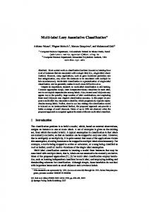
Science, Services, Shopping, Society, and Sports). Cadˆe has a vocabulary of 191,962 unique words. Information about the links related to the Cadˆe pages was also collected from the TodoBR collection. We refer to pages in TodoBr collection not classified in Cadˆe as external pages. Cadˆe has a total of 3,830 internal links, 554,592 links pointed to by external pages, and 5,584 links pointing to external pages. The second collection, which is called ACM8, was extracted from the first level of the ACM Computing Classification System (http://portal.acm.org/dl.cfm/). ACM8 is a set of 6,682 documents (metadata records) labelled using the 8 first level categories of ACM (General Literature, Hardware, Computer Systems Organization, Software, Data, Theory of Computation, Mathematics of Computing, Information Systems, Computing Methodologies, Computer Applications, Computing Milieux)2 . Only 55.80% of these documents have abstracts, which makes it very hard to classify them using traditional content-based classifiers. For the remaining documents, the only available textual content is title. But titles contain normally only 5 to 10 words. As a result, ACM8 has a vocabulary of just 9,840 unique words. ACM8 has a total of 11,510 internal citations and 40,387 citations for papers outside of ACM DL. The third collection, WebKB, consists of 8,282 Web pages collected from computer science departments of various universities in January 1997 by the World Wide Knowledge Base project (http://www.cs.cmu.edu/∼webkb/). All pages were manually classified into seven categories (student, faculty, staff, department, course, project, and other). MIME headers, HTML tags, and tokens that only occur once were discarded. Further, for each train/test split, we performed feature selection by removing all but the 2,000 words with highest mutual information with the class variable. WebKB has a total of 10,919 links between pages of the universities. Figure 1 shows the category distribution for the three collections. As we can see, the three collections have very skewed distributions. In Cade12, the three most popular categories represent more than 50% of all documents. The ACM8 collection has similar features, with the two most popular categories counting for more than a half of all documents in the collection. The more skewed collection, however, is WebKB. In this collection, the most popular class contains half of the pages. Note that, for the three collections, each document is classified into just one category. In all experiments with the aforementioned collections, we used 10-fold cross-validation and the final results of each experiment represent the average of the ten runs. We quantify the classification effectiveness of the various approaches through the conventional precision, recall and F1 measures. Precision p is defined as the proportion of correctly classified documents in the set of all documents. Recall r is defined as the proportion of correctly classified documents out of all the documents having the target category. F1 is a combination 2pr of precision and recall defined as the harmonic mean p+r . Macro- and micro-averaging [22] were applied to F1 to get single performance values over all classification tasks. For F1 macro-averaging (M acF1 ), scores were first computed for individual categories and then averaged over all categories. For F1 micro-averaging (M icF1 ), the decisions for all cate2 The three remaining categories of the ACM taxonomy, namely General Literature, Data and Computer Applications, had too few documents which prevented us to use them in our experiments.

ACM8

1

2

3

4

5

6

7

8

9 10 11 12

WebKB

2000 1800 1600 1400 1200 1000 800 600 400 200 0

3500 3000

# documents

# documents

# documents

Cade12 10000 9000 8000 7000 6000 5000 4000 3000 2000 1000 0

2500 2000 1500 1000 500 0

1

2

Categories

3

4

5

6

7

8

1

2

Categories

3

4

5

6

7

Categories

Figure 1: Category Frequency Distribution. gories were counted in a joint pool. The computational efficiency is evaluated through the total execution time, that is, the processing time spent in training and classifying all documents. We set σmin =0.001, θmin =0.975, βmin =0.800, ωmin =0.750, and αmin =0.700. The experiments were performed on a Linux-based PC with a Intel Pentium III 1.0 GHz processor and 1.0 GBytes RAM. All the results to be presented were found statistically significant at the 99% confidence level when tested with the two-tailed paired t-test.

5.1 Classification Effectiveness We start our analysis by evaluating the effectiveness of our method for different combinations of evidence (text, inlinks, and outlinks) and criteria (θ, β, ω, and α). Table 2 shows M icF1 numbers for each configuration used. With exception of the WebKB collection, textual information (t) performs poorly when compared against in-links (i) and out-links (o). In the Cade12 collection, text-based classifiers presented a very weak performance when compared with the results from ACM8 and WebKB collections. This is due to the fact that Web pages are usually noisy and contain little text. Further, due to issues such as multiple authorship, Web pages lack coherence in style, language, and structure. These problems are less common in the papers of a Digital Library. As a result, the quality of the textual evidence in ACM8 is better than in Cade12, but still not as good as the citation based information. In the case of WebKB, the good performance of textual classifiers is due to the skewness of the collection. A simple strategy of assigning the majority category to the test document is enough to ensure accuracy figures greater than 70%. In the three collections, textual evidence is a valuable source of information when combined with other types of evidence (i+t, o+t). Combining all available evidence (i+o+t) showed to be the best strategy for all collections. The combination of multiple evidence may lead to deeper understanding of the document than when only taking a single evidence into account. However, not all evidence are relevant and of good quality. Taking irrelevant or poor quality evidence into account may deteriorate the accuracy. For instance, in some cases the combination of different linkage evidence (i+o) did not show good accuracy results for the WebKB collection. As expected, different results were obtained from each criterion. In general, two-way confidence (ω) gives the best results, while weighted confidence (β) generally gives the worst results. The main reason for this is that only β is the one that uses the complement factor (c). However, this factor helped in classifying documents provenient from very low frequent classes in the WebKB collection. Combining different criteria also shows great improvements. For Cade12

Criteria θ β α ω θ+β θ+α θ+ω β+α β+ω α+ω θ+β+α θ+β+ω θ+α+ω β+α+ω θ+β+α+ω

t 54.18 50.48 53.25 52.83 53.01 55.37 55.00 52.72 52.40 55.12 55.26 55.41 56.34 54.22 56.02

i 71.78 70.04 72.30 72.81 69.16 72.79 73.07 69.42 69.17 73.21 71.25 71.42 73.36 71.20 71.58

o 73.61 71.93 73.96 74.22 73.63 74.48 74.76 73.68 73.77 75.64 73.99 74.06 75.05 74.11 74.52

Criteria θ β α ω θ+β θ+α θ+ω β+α β+ω α+ω θ+β+α θ+β+ω θ+α+ω β+α+ω θ+β+α+ω

t 62.42 61.76 62.95 63.02 62.88 63.27 63.13 63.13 62.60 63.45 63.24 63.22 62.85 62.43 63.68

i 71.36 70.01 72.12 71.93 71.06 73.24 72.26 71.77 71.52 74.83 73.31 73.05 75.90 74.97 75.54

o 72.68 71.33 72.94 72.73 72.63 73.53 73.05 72.87 72.76 75.27 74.27 74.03 76.60 75.34 76.22

Criteria θ β α ω θ+ω θ+β θ+α β+ω β+α α+ω θ+β+α θ+β+ω θ+α+ω β+α+ω θ+β+α+ω

t 81.15 81.82 80.19 81.06 81.36 81.28 80.03 81.88 80.39 81.01 82.51 82.86 82.80 82.66 82.97

i 70.81 70.99 70.60 70.45 71.82 72.18 71.96 72.51 72.04 71.87 73.17 73.92 72.82 72.98 73.60

o 74.17 74.58 74.29 74.70 76.44 75.69 75.12 76.51 75.33 75.28 76.55 77.10 76.83 76.17 76.91

Cade12 i+t 73.82 72.03 74.06 74.33 73.87 74.82 74.82 74.03 73.99 75.93 74.18 74.56 76.16 74.30 75.74 ACM8 i+t 74.26 73.69 74.79 74.95 73.65 74.55 74.92 74.08 74.28 75.50 77.85 76.26 79.65 77.38 79.85 WebKB i+t 78.25 78.62 77.38 78.84 79.47 79.35 78.16 79.58 79.08 78.06 79.75 79.36 80.13 79.59 80.58

o+t 75.26 73.16 75.41 75.68 73.55 75.80 75.85 75.08 75.08 76.55 75.62 75.53 77.79 75.35 77.09

i+o 76.93 74.82 77.07 77.25 75.84 77.91 78.04 76.14 76.14 77.43 76.41 76.41 78.92 76.49 78.01

i+o+t 77.15 75.32 78.13 78.41 77.19 78.80 78.80 77.46 77.61 78.98 77.73 77.73 80.41 77.84 79.59

o+t 74.39 74.00 75.66 75.64 73.95 74.98 75.47 75.22 75.29 75.68 78.25 80.76 82.15 81.49 82.52

i+o 77.55 76.24 78.04 77.77 76.50 78.86 79.21 78.41 78.74 79.72 79.97 81.81 83.80 82.19 83.12

i+o+t 79.13 77.79 80.34 80.64 79.06 81.57 82.10 81.27 81.60 82.42 81.90 82.96 85.15 82.51 83.22

o+t 79.82 80.01 79.72 80.37 80.56 80.28 78.70 80.52 79.51 79.11 81.19 81.97 81.49 81.82 82.12

i+o 73.68 74.32 73.40 75.02 76.83 76.18 75.90 77.37 77.13 77.02 77.17 78.21 77.01 78.07 78.58

i+o+t 80.66 81.22 78.37 81.71 81.96 81.84 79.60 82.44 79.92 80.09 82.17 83.52 82.35 82.68 83.04

Table 2: Different Evidence and Criteria. Degree 0 1 2 3

Cade12 M icF1 M acF1 56.64 59.75 80.41 81.94 76.28 77.52 67.12 68.34

ACM8 M icF1 M acF1 62.85 57.14 85.15 84.12 90.55 89.83 86.60 85.12

WebKB M icF1 M acF1 82.86 46.95 83.52 49.12 80.27 45.66 77.02 41.27

Table 3: Link Forwarding and Backwarding.

Coll. Cade12

ACM8

WebKB

Methods Co-citation kNN(text) SVM(text) Assoc.(eager) kNN(multi) SVM(multi) Bayesian Assoc.(lazy) Amsler SVM(multi) kNN(text) Assoc.(eager) SVM(text) kNN(multi) Bayesian Multi-Kernel Assoc.(lazy) SVM(text) kNN(multi) kNN(text) Multi-Kernel Assoc.(eager) Bayesian SVM(multi) Assoc.(lazy)

M icF1

M acF1

68.51 50.18 54.18 63.22 71.80 75.45 76.51 80.41 83.20 72.49 73.45 76.57 76.95 83.33 84.75 85.87 90.55 82.69 60.07 60.24 73.29 76.39 82.78 82.85 83.52

75.60 44.50 48.41 66.90 75.26 73.54 79.29 81.94 78.29 80.49 67.80 69.25 70.57 77.39 79.58 81.25 89.83 51.14 32.41 32.77 13.31 38.19 53.61 50.80 49.12

Gains (%) over baselines M icF1 M acF1 – – -26.7 -41.1 -20.9 -36.0 -7.7 -11.5 4.8 -0.4 10.1 -2.7 11.7 4.9 17.4 8.0 – – -12.9 2.8 -1.7 -13.4 -7.9 -11.5 -7.5 -9.9 0.1 -1.1 1.9 1.6 3.2 3.7 8.8 13.0 – – -27.3 -35.8 -27.1 -36.2 -11.4 -74.0 -7.6 -25.3 0.1 4.8 0.2 -0.6 1.00 -3.9

Table 4: Comparison against Different Approaches.

and ACM8 collections, the best configuration uses criteria θ, α, and ω, while for WebKB collection, the best configuration uses θ, β and ω. Hence, for now on we will use the configuration (i+o+t – θ+α+ω) (for Cade12 and ACM8 collections), and (i+o+t – θ+β+ω) (for WebKB collection), for the remaining experiments in this section. We continue our analysis by evaluating the link forwarding/backwarding approach. Table 3 shows M icF1 and M acF1 numbers for different degrees of relationships between the documents. For instance, degree 0 means that only textual information within the given document was used. Degree 1 means that we are also allowed to use in-links and out-links of the given document. Degree 2 means that we are also allowed to use in-links/out-links of documents that point to (or that are pointed by) the given document. Different results were obtained for the three collections. For the Cade12 and WebKB collections, the bests results (80.41%, and 83.52%) were achieved using only one degree of relationship, while for the ACM8 the best result (90.55%) was achieved when the second degree of relationship was also explored. This was due to the inherent differences between links and citations. Citations are used to provide background information, give credit to other authors, report or criticize similar ideas, among others. Besides all the functionality of citations, links have extra roles such as advertising, providing access to databases, navigation etc. Such roles can make them a less reliable source of evidence leading to noise in the classification process We used the best results obtained by our method and compare them with the best results obtained by carefully hand-tuned state-of-art single and multi-evidence methods. SVM[18] is the best known text-based classifier and therefore a standard baseline. Co-citation[17] and Amsler[1] are two bibliographic similarity measures that, when applied within a k-Nearest-Neighbor (kNN)[21] algorithm, produce classifiers whose performance is far superior than any textbased classifier in these collections, the former being the

best measure for Cade12 and the latter the best one for ACM8. Bayesian[4] and Multi-Kernel [11] are two state-ofthe-art representatives of the multiple experts and multiple evidence approaches. Given the huge size of the combined kernel matrix (about 500 million points for a symmetric sparse representation) we were not able to compute the multi kernel method for Cade12. Finally, since our method deals with text and link evidence in the same way, we also represent the documents to be classified as bags of features in which the features can be words and links taken indistinctly. Our last two multi-evidence approaches, SVM(multi) and kNN(multi), consist in classifying these documents using kNN and SVM classifiers, respectively. Table 4 depicts M icF1 and M acF1 numbers obtained for each method. Co-citation, Amsler, and SVM(text), were used as our baselines because they give good results when considered in isolation. The first entry for each collection is used as the baseline, and subsequent entries are sorted according to M icF1 . Text-based (SVM) and link-based classifiers present very distinct classification performance. Multievidence methods (Bayesian, multi-evidence kNN, multievidence SVM, Multi-Kernel and Associative) show the best classification performance, our method being clearly the best performer in all collections. The gains over the baseline are up to 17% depending to the collection. On the other hand, its eager counterpart performed poorly in all collections, and this is mainly due to the missing rule problem (many irrelevant rules, and only few relevant, were generated). Recall Bayes.

Docs per Class

Assoc. (lazy)

20.6% 17.6% 13.6% 11.1% 7.8% 6.9% 5.9% 5.2% 4.7% 2.7% 2.1% 1.8%

75.83 74.26 83.52 73.81 87.46 86.09 80.41 76.26 91.13 87.00 88.26 94.45

86.93 70.49 82.78 63.60 76.72 81.40 67.33 63.32 84.16 80.51 70.41 81.78

27.6% 23.2% 15.9% 10.5% 9.9% 6.4% 3.6% 2.9%

92.47 96.59 93.71 91.17 84.50 74.05 80.59 71.57

91.50 94.46 88.54 82.19 71.58 60.71 62.87 54.82

73.8% 13.4% 5.8% 3.7% 2.1% 1.1% 0.1%

89.31 63.80 95.88 73.86 10.47 30.43 0.00

90.1 63.8 67.5 77.8 44.2 2.2 5.0

Gain (%) Cade12 -12.8 5.3 0.9 16.0 14.0 5.8 19.4 20.4 8.3 8.0 25.3 15.5 ACM8 1.1 2.2 5.8 10.9 18.0 21.9 28.2 30.5 WebKB -0.87 0.0 42.0 -5.0 -76.3 1283.2 -100.0

Assoc. (lazy)

Precision Bayes.

Gain (%)

81.83 64.49 83.97 85.24 88.37 85.02 77.13 81.96 88.91 81.12 81.58 84.80

64.32 66.24 83.02 82.94 92.07 88.16 82.46 88.65 92.57 92.32 90.65 91.07

27.2 -2.6 1.1 2.7 -4.0 -3.5 -6.4 -7.5 -3.9 -12.1 -10.0 -6.9

88.45 93.63 95.32 90.01 85.67 82.28 84.09 89.24

78.46 86.50 93.00 89.18 83.51 79.69 93.12 87.10

12.7 8.2 2.5 0.9 2.6 3.2 -9.7 2.4

90.22 98.89 52.95 48.29 56.25 87.50 0.00

89.23 73.40 65.86 54.84 39.58 50.00 30.00

1.1 34.7 -19.6 -11.9 42.1 75.0 -100.0

Table 5: Comparison against Bayesian Combination. Table 5 shows detailed comparisons between our approach and the Bayesian combination approach (which was the most competitive performer). The table presents recall and precision figures for each category, considering all documents in the three collections. For Cade12, we observe a gain of 27%

in precision in the most frequent category, which is responsible for the overall gain in classification effectiveness. This is mainly due to the fact that the Bayesian combination approach uses the most frequent category in the training set as the fixed default prediction, which results in high recall and low precision numbers for more frequent categories. On the other hand, our approach uses the most frequent category in the projected training set. As a consequence, several documents that were misclassified by the Bayesian combination approach were correctly classified by our approach. Similarly to Cade12, the Bayesian combination approach prefers to assign documents to most frequent categories in WebKB. However, due to the skewness observed in this collection, this simple strategy leads to high gains. For ACM8 we observe more impressive gains in both precison and recall. The less frequent the category, the more is the gain in recall, and consequently, the opposite trend is observed in precision. In this case, the gains are mainly due to the link forwarding/backwarding technique, as previously observed in Table 3. Thus, instead of applying a fixed default prediction, our method performs link enhancement, which is succesful in this case because of the citation regularity observed in the ACM8 collection.

5.2 Computational Efficiency The computational performance of our method was also evaluated. Table 6 depicts the execution times obtained by employing different cache sizes. We allowed the cache to store from 0 to 100,000 rules (approximately 82 MBytes), and for each storage capacity we obtained the corresponding execution time. As expected, execution time is sensitive to cache size, showing improvements of about 200% for larger cache sizes. Similar trends were observed in all collections. Further, higher execution times were observed when textual evidence is used. This is explained by the fact that there is much more textual evidence than link-based evidence, and thus the number of rules based on textual information is much higher than the number of rules based on linkage information. Classification is extremely fast if only linkage evidence is used. For instance, our method is able to perform all ten folds of the ACM8 collection within two minutes. Coll. Cade12

ACM8

WebKB

Cache Size 0 1K 10K 100K 0 1K 10K 100K 0 1K 10K

t 2272 1638 1138 616 1611 1402 1032 562 1281 826 599

i 216 159 96 74 120 104 82 62 71 64 58

o 228 177 122 91 177 151 116 84 101 88 72

i+t 1926 1521 1048 535 1441 1251 936 501 1023 789 563

o+t 2261 1644 1129 598 1707 1501 1102 603 1211 806 593

i+o 485 381 246 131 417 342 239 126 184 138 117

i+o+t 2371 1827 1392 873 1927 1664 1276 704 1381 917 620

Table 6: Caching and Execution Times(secs). Table 7 shows the comparison between different methods. Lazy approaches learn quickly but classify slowly, while eager appoaches learn slowly but classify quickly. However, the use of caching is extremely useful for speeding up lazy classification. Only the Co-citation method was faster than ours in the Cade12 collection. Its effectiveness, however, was much worse than ours. Our method was the best performer in the ACM8 and WebKB collections. Its eager counterpart, on the other hand, spent much time generating a large

Collection Cade12

ACM8

WebKB

Method SVM(text) Bayesian SVM(multi) Associative(eager) Associative(lazy) Amsler Co-citation Multi-Kernel Bayesian SVM(multi) SVM(text) Associative(eager) Co-citation Amsler Associative(lazy) Multi-Kernel SVM(text) SVM(multi) Associative(eager) Associative(lazy)

Time ≈20 hours ≈20 hours ≈4.5 days ≈5,220 secs ≈870 secs ≈820 secs ≈790 secs ≈4.1 hours ≈2.3 hours ≈2 hours ≈2 hours ≈2,350 secs ≈1,200 secs ≈1,200 secs ≈700 secs ≈5.5 hours ≈5 hours ≈4 hours ≈5,280 secs ≈620 secs

M icF1 54.18 76.51 71.80 63.22 80.41 68.56 68.51 85.87 84.75 72.49 76.95 76.57 61.60 83.20 90.55 73.29 82.69 82.85 76.39 83.52

Table 7: Performance Comparison.

number of irrelevant rules (i.e., rules that were not used to classify any document in the test set), hurting the computational performance. Finally, we analyzed the sensitivity of our method by varying the ranking size, k (i.e., the number of rules within each ranking). The analysis was carried in terms of execution time and accuracy, which are depicted in Table 8. As expected, the execution time increases for larger ranking sizes, since more rules have to be generated in order to complete the ranking. Further, we notice that large increases and decreases of the ranking lead to low accuracy. This is due to the fact that larger rankings require more rules to be induced, and the direct consequence of applying our level-wise rule induction is that longer (and more specific) rules will be induced. We can see this by analyzing the average rule size column in Table 8, which clearly increases with the ranking size. By using a large number of specific rules, the classifier tends to overfit the data hurting the accuracy. On the other hand, by using only a low number of general rules, the classifier will underfit the data also hurting the accuracy. Thus, the choice of the proper ranking size is a trade-off between underfitting and overfitting.

6.

CONCLUSIONS

In this paper we propose and evaluate a novel document classification method which introduces innovations in all main steps of the automatic classification task. First, we propose a lazy method, which delays the model induction process until a new document is given for classification, incurring not only in classification accuracy gains, but also in performance improvement. Our lazy approach also performs evidence enhancement by looking forward/backward new pieces of link-based evidence in the citation/link graph. Second, we present a technique in which all evidence is treated within a unique search/classification space in a natural and transparent way. The pieces of evidence that enter in our classification model, independently of its type, are the ones that are more discriminative of the categories in which they occur according to our quality criteria. Finally, multiple quality criteria are combined in order to choose the best rules to be used to predict the correct category. Experimental results demonstrated that these innovations combined

Collection Cade12

ACM8

WebKB

Ranking Size (k) 10 15 20 25 30 35 40 10 15 20 25 30 35 40 10 15 20 25 30 35 40

Time (secs) 278 581 876 993 1109 1147 1232 403 673 704 746 793 853 979 481 573 623 685 817 889 1076

M icF1 77.33 78.60 80.41 80.78 80.99 80.69 80.10 86.64 88.83 90.55 90.21 90.29 90.06 88.28 80.48 81.83 83.52 81.77 82.05 80.27 78.69

Avg. Rule Size 2.25 3.09 3.62 3.91 4.27 4.35 4.72 2.91 3.72 4.03 4.29 4.52 4.68 4.91 2.78 3.22 3.46 3.75 4.11 4.66 4.93

Table 8: Ranking and Classification Performance. together produce more effective and faster classifiers than state-of-the-art approaches in the collections used, achieving more than 90% accuracy in some cases. As future work, we intend to design and evaluate novel rank criteria and combination strategies for these rankings. We want also to consider evidence weighting strategies, during the whole process. Finally, we will explore application scenarios such as bioinformatics and spam detection.

7. ACKNOWLEDGEMENTS This research was sponsored by UOL (www.uol.com.br) through its UOL Bolsa Pesquisa program (process number 20060519184000a). Additional support was provided by the 5S-QV project (grant MCT/CNPq/CT-INFO 55.1013/20052), Fucapi Technology Foundation, NSF Career Award IIS0092978, DOE Early Career Award DE-FG02-02ER25538 and NSF grants EIA-0103708, and EMT-0432098.

8. REFERENCES [1] R. Amsler. Application of citation-based automatic classification. Technical report, The University of Texas at Austin, Linguistics Research Center, 1972. [2] L. Breiman, J. Friedman, R. Olshen, and C. Stone. Classification and regression trees. Wadsworth Intl., 1984. [3] S. Brin, R. Motwani, and C. Silverstein. Beyond market baskets: Generalizing association rules to correlations. In Proc. of the ACM SIGMOD97, pages 265–276, May 1997. [4] P. Calado, M. Cristo, E. Moura, N. Ziviani, B. Ribeiro-Neto, and M. Gon¸calves. Combining link-based and content-based methods for web document classification. In Proc. of the ACM CIKM03, pages 394–401, 2003. [5] D. Cohn and T. Hofmann. The missing link - A probabilistic model of document content and hypertext connectivity. In Advances in Neural Inf. Processing Systems, pages 430–436. MIT Press, 2001. [6] S. Dasgupta, M. Littman, and D. McAllester. PAC generalization bounds for cotraining. In Proc. of Neural Inf. Processing Systems, 2001.

[7] M. Fisher and R. Everson. When are links useful? Experiments in text classification. In Proc. of ECIR03, pages 41–56, Pisa, Italy, April 2003. [8] J. Friedman, R. Kohavi, and Y. Yun. Lazy decision trees. In Proc. of the Nat. Conf. on Artificial Intelligence, pages 717–724, Menlo Park, 1996. [9] J. Furnkranz. Exploiting structural information for text classification on the WWW. In Proc. of the IDA99, pages 487–498, Amsterdam, August 1999. [10] D. Gibson, J. M. Kleinberg, and P. Raghavan. Inferring Web communities from link topology. In Proc. of the ACM Conf. on Hypertext and Hypermedia, pages 225–234, Pittsburgh, PA, USA, June 1998. [11] T. Joachims, N. Cristianini, and J. Shawe-Taylor. Composite kernels for hypertext categorisation. In Proc. of the ICML01, pages 250–257, June 2001. [12] W. Li, J. Han, and J. Pei. CMAR: Efficient classification based on multiple class-association rules. In Proc. of the ICDM01, pages 369–376, 2001. [13] B. Liu, W. Hsu, and Y. Ma. Integrating classification and association rule mining. In Knowledge Discovery and Data Mining, pages 80–86, 1998. [14] J. Quinlan. C4.5: Programs for machine learning. Morgan Kaufmann, 1993. [15] F. Sebastiani. Machine learning in automated text categorization. ACM Comp. Surveys, 34(1):1–47, 2002. [16] A. Silva, E. Veloso, P. Golgher, B. Ribeiro-Neto, A. Laender, and N. Ziviani. CobWeb - a crawler for the Brazilian Web. In Proc. of the SPIRE99, pages 184–191, 1999. [17] H. Small. Co-citation in the scientific literature: A new measure of relationship between two documents. JASIS, 24(4):265–269, 1973. [18] A. Sun, E.-P. Lim, and W.-K. Ng. Web classification using support vector machine. In Proc. of the Intl. Work. on Web Inf. and Data Management, pages 96–99, USA, Nov. 2002. [19] P. Tan, V. Kumar, and J. Srivastava. Selecting the right interestingness measures for association patterns. In Proc. of the ACM SIGKDD02, pages 32–41, 2002. [20] L. Terveen, W. Hill, and B. Amento. Constructing, organizing, and visualizing collections of topically related web resources. ACM Trans. Computer-Human Interaction., 6(1):67–94, March 1999. [21] Y. Yang. Expert network: Effective and efficient learning from human decisions in text categorization and retrieval. In Proc. of the ACM SIGIR94, pages 13–22, Dublin, Ireland, July 1994. [22] Y. Yang, S. Slattery, and R. Ghani. A study of approaches to hypertext categorization. Journal of Intell. Inf. Systems, 18(2–3):219–241, 2002. [23] X. Yin and J. Han. CPAR: Classification based on predictive association rules. In Proc. of the SDM03. SIAM, 2003. [24] M. Zaki and C. Aggarwal. XRules: An effective structural classifier for XML data. In Proc. of the ACM SIGKDD03. ACM Press, 2003. [25] B. Zhang, Y. Chen, W. Fan, E. Fox, M. Gon¸calves, P. Calado, and M. Cristo. Intelligent GP fusion from multiple sources for text classification. In Proc. of the CIKM05, 2005.