Multi-GPU, Implicit Time Stepping for High-order Methods on ...

AIAA 2016-3965 AIAA Aviation 13-17 June 2016, Washington, D.C. 46th AIAA Fluid Dynamics Conference

Multi-GPU, Implicit Time Stepping for High-order Methods on Unstructured Grids Jerry Watkins∗, Joshua Romero∗, and Antony Jameson† Department of Aeronautics and Astronautics, Stanford University, Stanford, CA, 94305

In this paper, the development, implementation and performance of a multi-GPU, implicit, high-order compressible flow solver for unstructured grids is discussed. The solver utilizes the direct Flux Reconstruction (DFR) method and a multicolored Gauss-Seidel (MCGS) method to converge the steady state Euler equations in a multi-GPU environment. The MCGS scheme is able to obtain a fast, grid converged lift coefficient of 0.1795 for the NACA 0012 airfoil at a 1.25 degree angle of attack, Mach 0.5. The results are obtained with fewer degrees of freedom when compared to Overflow and CFL3D. The high arithmetic intensity and the ease of parallelization makes MCGS an ideal choice for multiple GPUs. The memory size of the left-hand side matrices in the implicit method limits the scheme’s use for high polynomial orders on a single GPU but it is shown that the bottleneck in memory usage can be mitigated by using multiple GPUs. The scheme is able to maintain near perfect weak scaling showing that it can be effectively distributed over multiple GPUs to solve large problems without a significant degradation in performance.

I.

Introduction

Significant contributions have been made towards progressing high-order methods in computational fluid dynamics (CFD). High-order methods refer to a branch of numerical algorithms which employ higher than second order spatial discretization. These algorithms can improve the accuracy of a simulation at a reduced computational cost.1 In the past, these methods have failed to penetrate the computational design process because they are generally less robust and more complex to implement than commonly used low-order methods. In recent years, these disadvantages have been mitigated and high-order methods are becoming increasingly more popular in the study of steady and unsteady, vortex dominated flows over complex geometries. These flows are often more difficult to simulate using low-order methods because of the high computational cost and increased sensitivity to geometry and numerical dissipation. Discontinuous finite element methods have been the focal point of recent efforts in developing a highorder compressible flow solver for unstructured grids. Popular examples include the Discontinuous Galerkin (DG) scheme2–4 and the Spectral Difference (SD) scheme.5, 6 Huynh7 proposed a Flux Reconstruction (FR) approach for tensor-product elements that provides a generalized differential framework for recovering both the collocation based nodal DG scheme as well as a version of the SD scheme. This framework has been successfully extended to triangular8, 9 and tetrahedral10 elements as well. Even more general frameworks such as the Correction Procedure via Reconstruction (CPR)11 have now been proposed that unify the FR and the Lifting Collocation Penalty (LCP)12 formulations. Recently, the direct Flux Reconstruction (DFR) method has been developed as a simplified formulation of the FR method that reduces the theoretical and implementation complexity of the FR method.13 The push towards high-order, unsteady flow simulations over complex geometries has sparked a need for faster convergence for large scale problems. Accelerated explicit methods and the polynomial multigrid method have been used to accelerate convergence rates but are sometimes not enough to overcome the stiffness found in aerodynamic applications where the cell volume varies by several orders of magnitude between the body and the far field.14–16 For these class of problems, implicit methods offer an alternate means to converge steady state solutions or drive the solution to physical time steps in dual time stepping ∗ Ph.D.

Candidate, Department of Aeronautics and Astronautics, Stanford University, AIAA Student Member Department of Aeronautics and Astronautics, Stanford University, AIAA Member

† Professor,

1 of 33 American Institute of Aeronautics and Astronautics Copyright © 2016 by Jerry Watkins, Joshua Romero, Antony Jameson. Published by the American Institute of Aeronautics and Astronautics, Inc., with permission.

methods by means of larger pseudo time steps. In particular, lower-upper symmetric Gauss-Seidel (LU-SGS) has shown promising results in unstructured compressible flow solvers utilizing finite volume methods, SD methods, the CPR method and more recently, the compact high-order method.16–20 Graphical Processing Units (GPUs) are also becoming more popular among those in the scientific computing community and can demonstrate a substantial performance gain for programs using high-order methods.14, 15, 19, 21, 22 The DFR method is well suited for GPUs because the vast majority of operations are element local and the increase in amount of work per degree of freedom couples well with the high computational potential of GPUs. Castonguay et al. has shown the potential of these accelerators to produce results for unsteady simulations using explicit time stepping.14 Typically, implicit time stepping has been a more difficult problem to address because of the increase in memory requirements and the serial aspects of the algorithm but there have been advances which show that there are methods of overcoming these problems on a single GPU.19 In this paper, a multi-GPU high-order compressible flow solver for unstructured grids is developed and used to perform implicit time stepping on steady Euler problems. The paper is formatted as follows. Section II gives a detailed overview of the DFR method on one-dimensional, two-dimensional quadrilateral and triangular elements and the Euler equations. Section III gives an overview of the explicit RK44 method, the implicit Multicolored Gauss-Seidel (MCGS) method and a description of the analytical implicit Jacobian used in the implicit method. Section IV discusses the implementation details of the explicit and implicit method on a multi-GPU system. Section V provides two numerical tests which verify that the MCGS method produces accurate results. Lastly, Section VI provides an overview of the speedup of the GPU implementation over the CPU implementation and a strong and weak scalability analysis of the multi-GPU implementation.

II.

Direct Flux Reconstruction Method

In this section, a detailed overview of the DFR method is provided. In previous work, this scheme has been proven capable of recovering the FR form of the nodal DG method with a simplified procedure relative to the existing FR framework.13 The section begins with a description of the method applied to a one-dimensional scalar conservation law. This is followed by a description of the scheme applied to a two-dimensional scalar conservation law and Euler equations on quadrilateral and triangular elements. A. 1.

One-Dimensional Formulation Problem Specification

Consider the one-dimensional scalar conservation law, ∂u ∂f (u) + = 0, x ∈ Ω = [a, b], t > 0, (1) ∂t ∂x where x is the spatial coordinate, t is time, u = u(x, t) is a conserved scalar quantity and f = f (u) is the flux. An initial condition is specified and Dirichlet and Neumann boundary conditions are introduced on the left and right boundaries so that, u(x, 0) = u0 (x), u(a, t) = ua , ∂f (b, t) = 0. (2) ∂x Following a traditional nodal finite element method, the domain is partitioned into Neles non-overlapping elements, N[ eles Ω= Ωele , (3) ele=1

where Ωele = [xele , xele+1 ). With the domain partitioned, the exact solution u and the exact flux f (u) can be approximated by the numerical solution and the numerical flux, δ

u =

N eles X

uδele ,

δ

f =

ele=1

N eles X

δ fele .

ele=1

2 of 33 American Institute of Aeronautics and Astronautics

(4)

A linear isoparametric mapping is introduced from the physical domain x ∈ Ωele to the parent domain ξ ∈ ΩS = [−1, 1) such that x − xele − 1, ξ(x|Ωele ) = 2 xele+1 − xele 1−ξ 1+ξ x|Ωele (ξ) = xele + xele+1 . (5) 2 2 Applying this transformation gives rise to a transformed equation within the standard element ΩS of the following form δ 1 ∂ fêle ∂u ˆδele + = 0, (6) ∂t |Jele | ∂ξ where

u ˆδele = uδele (x|Ωele (ξ), t), fˆδ = f δ (x|Ω (ξ), t), ele

ele

ele

and |Jele | = 21 (xele+1 − xele ) is the determinant of the geometric element Jacobian matrix of the coordinate transformation. In what follows, the hat notation to denote the transformed solution and corresponding transformed flux will be dropped for brevity. 2.

Direct Flux Reconstruction

Consider the transformed semi-discrete equation for the one-dimensional scalar conservation law, δ 1 δfele ∂uδele =− , ∂t |Jele | δξ

(7)

δf δ

δ where δξele is the numerical derivative of fele . In the DFR method, a transformed globally C 0 continuous δ flux f δ is reconstructed in order compute the numerical derivative of fele in each element. The first step is to further discretize each element by Nspts1D = P + 1 distinct solution points so that the discontinuous solution in each element uδele can be represented by a piecewise interpolating polynomial of degree P , Nspts1D

uδele (ξ)

=

X

uδspt,ele `spt (ξ),

(8)

spt=1

where {`1 (ξ), . . . , `Nspts1D (ξ)} are the Lagrange polynomials defined at the solution points {ξ1 , . . . , ξNspts1D }. This can be written in vector format as, uδele (ξ) = `(ξ)T uδele ,

(9)

where `(ξ)T = [`1 (ξ), . . . , `Nspts1D (ξ)] and uδele = [uδ1,ele , . . . , uδNspts1D ,ele ]T . To recover the nodal DG method, the solution points are chosen to be collocated with the zeros of the Legendre polynomial of degree P + 1, also known as the Gauss-Legendre points.13 The next step is to extrapolate the discontinuous solution to the element interfaces using Eq.(9). The extrapolated values in each element are written as, uδele (−1) = `(−1)T uδele , uδele (+1) = `(+1)T uδele .

(10)

The transformed common interface fluxes are computed by using the extrapolated discontinuous solution on both sides of each interface as the left and right states in an appropriate numerical flux formulation for the equation being solved. The transformed common interface fluxes are written as δ,W fele = f I (uδele−1 (+1), uδele (−1)), δ,E fele = f I (uδele (+1), uδele+1 (−1)),


(11)

δ,W δ,E where f I (uL , uR ) is the interface flux function and fele and fele are the transformed common interface th fluxes on the west and east boundaries of the ele element, respectively. A Riemann solver is commonly used as the interface flux function. In this paper, the Rusanov flux is computed so that 1 1 f I (uL , uR ) = (f (uR ) + f (uL )) − |λ(uL , uR )|(uR − uL ), (12) 2 2 where ∂f ∂f (13) |λ(uL , uR )| = max (uR ) , (uL ) , ∂u ∂u ∂f and ∂u (u) is the wavespeed or the derivative of the flux with respect to the solution. The transformed common interface fluxes at Dirichlet and Neumann boundaries are computed by using the boundary conditions specified in Eq.(2),

Dirichlet BC: f1δ,W = f (ua ), Neumann BC:

δ,E fN = f (uδNeles (1)), eles

(14)

δ The next step is to construct a transformed continuous flux fele such that a piecewise sum results in 0 δ a transformed globally C continuous flux, f , that passes through the transformed common interface flux values at element interfaces. This is accomplished using the following Lagrange interpolant, Nspts1D δ fele (ξ)

=

δ,W ˜ fele `0 (ξ)

X

+

δ,E ˜ δ fspt,ele `˜spt (ξ) + fele `P +2 (ξ),

(15)

spt=1

where {`˜0 (ξ), . . . , `˜P +2 (ξ)} are the Lagrange interpolating polynomials of degree P + 2 defined at P + 3 δ collocation points {−1, ξ1 , . . . , ξNspts1D , 1}, fspt,ele = f (uδspt,ele ) is the transformed flux evaluated at solution δ points and fele is the resulting transformed continuous flux. δ The final step is to obtain the numerical derivative of fele by differentiating Eq.(15) with respect to ξ and evaluating at each solution point, Nspts1D δ X ˜ ˜ ∂ `˜spt δfele δ,W ∂ `0 δ,E ∂ `P +2 δ (ξi ) = fele (ξi ) + fspt,ele (ξi ) + fele (ξi ). δξ ∂ξ ∂ξ ∂ξ spt=1

(16)

This can be manipulated into a matrix-vector format so that, δ δfele δ,W δ,E δ = DξW fele + Dξ fele + DξE fele , δξ

(17)

δ δ δ where fele = [f1,ele , . . . , fN ]T and Dξ ∈ R(Nspts1D ×Nspts1D ) and DξW , DξE ∈ R(Nspts1D ×1) are polynospts1D ,ele mial differentiation operators such that

∂ `˜m (ξp ), ∂ξ ∂ `˜0 = (ξp ), ∂ξ ∂ `˜P +2 = (ξp ), ∂ξ

Dξp,m = DξWp DξEp

p, m = 1, 2, . . . , Nspts1D , p = 1, 2, . . . , Nspts1D , p = 1, 2, . . . , Nspts1D .

(18)

This is coupled with Eq.(7) to obtain the transformed semi-discrete equation in vector format, δ ∂uδele 1 δfele =− . ∂t |Jele | δξ

B.

(19)

Two Dimensional Extension to Quadrilateral Elements

The DFR method, along with other Flux Reconstruction (FR) methods, can be directly extended to quadrilateral elements using a tensor-product formulation.7 While the cited references describe the methodology in the context of the standard FR method, the same procedure can be applied to the DFR method by simply replacing the FR correction procedure using correction polynomials with the Lagrange interpolation described by Eq.(15). A summary of the procedure is described below. 4 of 33 American Institute of Aeronautics and Astronautics

1.

Problem Specification

Consider the two-dimensional scalar conservation law, ∂u ∂f (u) ∂g(u) + + = 0, ∂t ∂x ∂y

(x, y) ∈ Ω,

t > 0,

(20)

where Ω is an arbitrary domain, x and y are the spatial coordinates, t is time, u = u(x, y, t) is a conserved scalar quantity and f = f (u) and g = g(u) are the fluxes in the x and y directions, respectively. An initial condition is specified and Dirichlet and Neumann boundary conditions are introduced on arbitrary S boundaries ∂ΩΘ and ∂ΩΦ , respectively, such that the entire boundary is ∂Ω = ∂ΩΘ ∂ΩΦ and, u(x, y, 0) = u0 (x, y), u(x, y, t) = uΘ (x, y), (x, y) ∈ ∂ΩΘ , ∂f n (x, y, t) = 0, (x, y) ∈ ∂ΩΦ , ∂n

(21)

where n is the direction normal to ∂ΩΦ and f n is the component of the flux along n. Following a traditional nodal finite element method, the domain is partitioned into Neles non-overlapping, conforming quadrilateral elements, N[ eles Ω= Ωele . (22) ele=1

Each quadrilateral element in the physical domain (x, y) is mapped to a reference element in the transformed parent space (ξ, η) so that, x y

!

Nnpts

xnpt,ele = Γele (ξ, η) = Mnpts (ξ, η) ynpt,ele npt=1

!

X

(23)

where Mnpts (ξ, η) are the element shape functions and Nnpts is the number of points used to define the physical space element.

x3,ele b

(−1, 1)

(1, 1)

b

b

b

b

x4,ele b

x = Γele (ξ, η)

y

η

b

x2,ele b

x1,ele

(1, −1)

(−1, −1) x

ξ

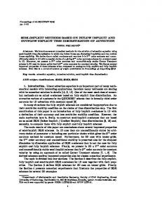
Figure 1: Mapping of physical space quadrilateral element to reference quadrilateral using mapping Γele (ξ, η) Applying this transformation gives rise to a transformed equation of the following form, ! δ δ ∂u ˆδele 1 ∂ fêle ∂ˆ gele + + = 0, ∂t |Jele | ∂ξ ∂η 5 of 33 American Institute of Aeronautics and Astronautics

(24)

where u ˆδele = uδele (Γele (ξ, η), t), ∂x δ ∂y δ δ f (Γele (ξ, η), t) − g (Γele (ξ, η), t), fêle = ∂η ele ∂η ele ∂x δ ∂y δ δ gêle = − fele (Γele (ξ, η), t) + g (Γele (ξ, η), t), ∂ξ ∂ξ ele ∂y ∂x ∂y and the terms, |Jele |, ∂η , ∂η , ∂ξ and ∂x ∂ξ are computed in each element from Eq.(23). In what follows, the hat notation to denote the transformed solution and corresponding transformed fluxes will be dropped for brevity.

2.


Consider the transformed semi-discrete equation for the two-dimensional scalar conservation law, δ δ ∂uδele 1 δfele δgele =− + , ∂t |Jele | δξ δη δf δ

(25)

δg δ

δ δ and gele , respectively. The DFR method for 2D where δξele and δηele are the numerical derivatives of fele quadrilateral elements is similar to the method for 1D. The first step is to further discretize each quadrilateral element by Nspts = (P +1)2 distinct solution points generated through a tensor product of a set of 1D solution points. Each solution point is defined by the sets {ξ1 , . . . , ξNspts1D } and {η1 , . . . , ηNspts1D }. The discontinuous solution in each element uδele can be represented by a product of piecewise interpolating polynomials of degree P, Nspts X δ uele (ξ, η) = uδspt,ele φspt (ξ, η), (26) spt=1

where φspt (ξ, η) = ì (ξ)`j (η) and ì (ξ) and `j (η) are 1D Lagrange polynomials defined at the sptth solution point located at (ξi , ηj ). This can be written in vector format as, uδele (ξ, η) = φ(ξ, η)T uδele ,

(27)

where φ(ξ, η)T = [`1 (ξ)`1 (η), . . . , `Nspts1D (ξ)`Nspts1D (η)] and uδele = [uδ1,ele , . . . , uδNspts ,ele ]T . The next step is to extrapolate the discontinuous solution to Nspts1D = P + 1 distinct flux points on each edge of a quadrilateral element for a total of Nfpts = 4Nspts1D flux points. Using Eq.(27), the extrapolated values in each element are written as, W uδ,W uδele , ele = E S δ uδ,S ele = E uele ,

E δ uδ,E uele , ele = E N uδ,N uδele , ele = E

(28)

δ,E δ,S δ,N (Nspts1D ×1) where uδ,W are the extrapolated discontinuous solution vectors on the west, ele , uele , uele , uele ∈ R east, south and north boundaries of the eleth element, respectively, as shown in Figure 2 and E W , E E , E S , E N ∈ R(Nspts1D ×Nspts ) are polynomial extrapolation operators such that W Ep,m = φm (−1, ηp ),

p = 1, 2, . . . , Nspts1D ,

m = 1, 2, . . . , Nspts ,

E Ep,m S Ep,m N Ep,m

= φm (+1, ηp ),

p = 1, 2, . . . , Nspts1D ,

m = 1, 2, . . . , Nspts ,

= φm (ξp , −1),

p = 1, 2, . . . , Nspts1D ,

m = 1, 2, . . . , Nspts ,

p = 1, 2, . . . , Nspts1D ,

m = 1, 2, . . . , Nspts ,

= φm (ξp , +1),

(29)

Transformed common interface fluxes that are normal to the element faces are computed by using the extrapolated discontinuous solution on both sides of each interface as the left and right states in a common interface function. The transformed common interface fluxes are written as δ,W δ,E δ,W I fele = dAW ele f (ueleN , uele ), δ,S δ,N δ,S I gele = dAS ele f (ueleN , uele ),

δ,E δ,E δ,W I fele = dAE ele f (uele , ueleN ), δ,N δ,N δ,S I gele = dAN ele f (uele , ueleN ),


(30)

N

R r

r

L r

b b

r

E

W L R

b

r

b

R r

L

L R r

r

S

Figure 2: A visual representation of a quadrilateral element in parent space for a polynomial order of P = 1. The solution points are marked by blue circles, the flux points are marked by red squares and west, east, south and north faces are represented by W, E, S, N , respectively. Left and right states in an interface flux are represented by L and R.

E S N (Nspts1D ×Nspts1D ) where ”eleN” refers to the neighboring element and dAW are diagele , dAele , dAele , dAele ∈ R onal matrices that transform the common interface fluxes such that W W −T W (Jele,p ) n ˆ , p = 1, 2, . . . , Nspts1D , dAW ele,p,p = Jele,p E E E −T E dAele,p,p = Jele,p (Jele,p ) n ˆ , p = 1, 2, . . . , Nspts1D , S S −T S S dAele,p,p = Jele,p (Jele,p ) n ˆ , p = 1, 2, . . . , Nspts1D , N N −T N N p = 1, 2, . . . , Nspts1D , (31) ˆ , dAele,p,p = Jele,p (Jele,p ) n N S E W , Jele,p are the geometric element Jacobian matrices evaluated at the pth flux point , Jele,p , Jele,p where Jele,p and n ˆW , n Ê, n ˆS, n ˆ N are the unit normals in parent space. The Rusanov flux used for the common interface function from Eq.(12) now becomes

f I (uL , uR ) =

1 n 1 (f (uR ) + f n (uL )) − |λ(uL , uR )|(uR − uL ), 2 2

(32)

where f n (u) is the flux normal to the face and n n ∂f ∂f |λ(uL , uR )| = max (uR ) , (uL ) , ∂u ∂u

(33)

n

where ∂f ∂u (u) is the wavespeed of the normal flux or the derivative of the normal flux with respect to the solution. The transformed common interface fluxes at Dirichlet and Neumann boundaries defined in Eq.(21) are computed as, Dirichlet BC: f δ,Θ = dAΘ f n (uΘ ), Neumann BC:

f δ,Φ = dAΦ f n (uδ,Φ ),

(34)

where uΘ is a vector of uΘ (x, y) evaluated at the boundary flux points, uδ,Φ is a vector of extrapolated solutions on the boundary flux points and dAΘ , dAΦ are diagonal matrices that transform the normal fluxes at the boundaries. 7 of 33 American Institute of Aeronautics and Astronautics

δ δ The transformed continuous fluxes in each element, fele and gele , are constructed such that they pass through the transformed common interface fluxes at flux points by using Lagrange interpolants. The numerical derivative of the transformed continuous fluxes evaluated at each solution point can then be written as Nspts1D Nspts1D Nspts1D δ X δ,W ∂ `˜0 X X ∂ `˜p δfele δ fele (ξp , ηm ) (ξi , ηj ) = fele,fpt (ξi ) `˜fpt (ηj ) + (ξi ) `˜m (ηj ) δξ ∂ξ ∂ξ p=1 m=1 fpt=1

Nspts1D δ,E fele,fpt

X

+

fpt=1

∂ `˜P +2 (ξi ) `˜fpt (ηj ), ∂ξ

Nspts1D

Nspts1D Nspts1D δ X δ,S X X δgele ∂ `˜0 ∂ `˜m δ ˜ (ξi , ηj ) = gele,fpt `fpt (ξi ) (ηj ) + gele (ηj ) (ξp , ηm ) `˜p (ξi ) δη ∂η ∂η m=1 p=1 fpt=1

Nspts1D

+

X fpt=1

∂ `˜P +2 δ,N (ηj ), gele,fpt `˜fpt (ξi ) ∂η

(35)

where {`˜0 (ξ), . . . , `˜P +2 (ξ)} and {`˜0 (η), . . . , `˜P +2 (η)} are the 1D Lagrange interpolating polynomials of degree P +2 defined at P +3 collocation points {−1, ξ1 , . . . , ξNspts1D , 1} and {−1, η1 , . . . , ηNspts1D , 1}, respectively, and ∂y ∂y ∂x δ δ δ δ δ f (uδele (ξp , ηm )) − ∂x fele (ξp , ηm ) = ∂η ∂η g(uele (ξp , ηm )) and gele (ξp , ηm ) = − ∂ξ f (uele (ξp , ηm )) + ∂ξ g(uele (ξp , ηm )) are the transformed fluxes evaluated at solution points. This can be manipulated into a matrix-vector format so that, δ δfele δ,W δ,E δ = DξW fele + Dξ fele + DξE fele , δξ δ δgele δ,S δ,N δ = DηS gele + Dη gele + DηN gele , δη

(36)

δ δ δ δ δ δ where fele = [f1,ele , . . . , fN ]T , gele = [g1,ele , . . . , gN ]T and Dξ , Dη ∈ R(Nspts ×Nspts ) and DξW , DξE , spts ,ele spts ,ele DηS , DηN ∈ R(Nspts ×Nspts1D ) are polynomial differentiation operators. This is coupled with Eq.(25) to obtain the transformed semi-discrete equation in vector format, δ ∂uδele 1 δfele δg δ =− + ele . (37) ∂t |Jele | δξ δη

3.

Extension of Tensor Product Formulation to Triangular Elements

The tensor product formulation of the DFR method on quadrilaterals can be directly extended to triangular elements using an edge-collapsing method.23 In the cited reference, the treatment of ghost flux points, defined as the flux points co-located at the collapsed vertex is discussed. For first-order fluxes, the common interface flux at these points is set to zero since there is no face area at these points. A visual depiction of these elements can be seen in Figure 3. C.

Euler Equations

1.

Problem Specification

Consider the unsteady, two-dimensional, Euler equations in conservative form,

   U = 

∂F ∂G ∂U + + = 0, ∂t ∂x ∂y     ρ ρu ρv     2 ρu  ρuv  ρu + p   , F =  , G =     ρv 2 + p ρv  ρuv e (e + p)u (e + p)v 8 of 33 American Institute of Aeronautics and Astronautics

(38)    , 

(39)

x3,ele

r

r

y

x4,ele

b rs

x1,ele

r b

r

rs

b

b r

rs

b

b r

r

r

x = Γele (ξ, η) b

b

r

r

r

η

r

x2,ele

x

ξ

Figure 3: Mapping of physical space triangular element to reference quadrilateral using mapping Γ(ξ, η). Hollow red squares depict interface ghost flux points.

where ρ is density, u, v are the velocity components in the x, y directions, respectively, and e is total energy per unit volume. The pressure is determined from the equation of state, 1 (40) p = (γ − 1) e − ρ u2 + v 2 , 2 where γ is the ratio of specific heats. 2.


The DFR method can be directly applied to Eq.(37) so the transformed semi-discrete equation becomes, δ δ δFele ∂Uele 1 δGδele =− + . (41) ∂t |Jele | δξ δη

The formulation of the discontinuous solution and the extrapolation procedure of the solution to flux points follows exactly as described in the previous section. The transformed common interface fluxes are also computed the same as before. For the Euler equations, the Rusanov flux used for the common interface function now becomes, 1 n 1 (F (UR ) + F n (UL )) − |λ(UL , UR )|(UR − UL ), 2 2 where F n (U ) is the flux normal to the face and F I (UL , UR ) =

|λ(UL , UR )| = max (|VRn | + cR , |VLn | + cL ) ,

(42)

(43)

where V n is the velocity normal to the face and c is the speed of sound. The boundary conditions used at the boundary faces are shown in the appendix. Following from Eq.(36), the numerical derivatives of the transformed continuous fluxes evaluated at each solution point for each variable can be written in a matrix-vector format. Consider arranging the numerical solution in each element into a vector of (Nspts × 1) values for each conservative variable so that Uele,var = [Uele,var,1 , Uele,var,2 , . . . , Uele,var,Nspts ]T where ”var” represents an index for a solution variable. The numerical derivative can then be written as, δ δFele,var δ,W δ,E δ = DξW Fele,var + DξD Fele,var + DξE Fele,var , δξ δGδele,var δ,N D δ N = DηS Gδ,S ele,var + Dη Gele,var + Dη Gele,var , δη


(44)

This can be applied directly to Eq.(41) so that the transformed semi-discrete equation in vector format becomes, ! δ δ δFele,var ∂Uele,var δGδele,var 1 =− + . (45) ∂t |Jele | δξ δη For the remainder of the paper, the delta notation to denote the numerical approximation of solution and flux will be dropped for brevity.

III.

Time-Stepping Schemes

The fully discrete equation in each element is obtained by substituting the exact time derivative term in Eq.(41) with the numerical time derivative, δUele = R(Uele , UeleN ), δt

(46)

where, 1 R(Uele , UeleN ) = − |Jele |

δFele δGele + δξ δη

,

(47)

and UeleN is the set of all neighboring solution point values needed for the residual R. A.

Explicit Method

An explicit, four-stage Runge-Kutta (RK) scheme is used to update the solution in all elements at each stage, Res(1) = R(U s ), Res(2) = R(U s + ∆t Res(1) ), 1 Res(3) = R(U s + ∆t Res(2) ), 2 1 (4) s Res = R(U + ∆t Res(3) ), 2 1 1 1 1 s+1 s U = U + Res(1) + Res(2) + Res(3) + R(U s + ∆t Res(4) ) 6 3 3 6

(48)

where ∆t is the numerical time step and the subscript ”ele” has been omitted to signify that the residual and update computations happen on all elements. A timestep based on the Courant-Friedrich-Lewy (CFL) condition can be computed as, ∆tele =

HCFL Vele

,

(49)

|λ| dA

∂Ωele

where Vele is the element volume and ∂Ωele refers to the element boundary. B.

Implicit Method

An implicit, backward Euler scheme is used to find the solution in each element at the next time step, s+1 s+1 ∆Uele = ∆t R(Uele , UeleN )

(50)

s+1 s+1 s+1 s where ∆Uele = Uele − Uele . A Taylor series expansion of R(Uele , UeleN ) is used to linearize the equation, s+1 s+1 s s R(Uele , UeleN ) ≈ R(Uele , UeleN )+

s X ∂Rs ∂Rele ele ∆Uele + ∆UeleN , ∂Uele ∂UeleN

(51)

eleN

s s s where Rele = R(Uele , UeleN ). Rearranging Eq.(50) by using the approximation in Eq.(51) gives the global linear system, s X ∂Rs I ∂Rele s s ele + ∆Uele − ∆UeleN = R(Uele , UeleN ). (52) ∆t ∂Uele ∂UeleN eleN


In order to parallelize the linear solver and eliminate the dependency of neighboring elements on the left-hand side matrix, a multicolored Gauss-Seidel (MCGS) algorithm is used, s X ∂Rs ∂Rele I k+1 ∗ s s ele + ∆Uele ∆UeleN (53) = R(Uele , UeleN )+ ∆t ∂Uele ∂UeleN eleN

k+1 ∗ where ∆Uele refers to the ∆U of an element with the current color and ∆UeleN refers to the most recently s+1 s updated ∆U of neighboring elements. The solution Uele is updated to Uele after all colors have been updated. For example, in a two color, red-black Gauss-Seidel the algorithm is: update ∆U on red elements, s update ∆U on black elements, update Uele on all elements. The right-hand side can be further reduced by using the following linear approximation, s ∗ s s R(Uele , UeleN ) ≈ R(Uele , UeleN )+

so that,

s I ∂Rele + ∆t ∂Uele

X ∂Rs ∗ ele ∆UeleN , ∂UeleN

(54)

eleN

k+1 s ∗ ∆Uele = R(Uele , UeleN ).

(55)

s The solution Uele must now be updated as soon as a color has been updated in order to compute a new residual. It’s also possible to perform a backsweep of all colors. In this case, the equation becomes s ∂Rele I k+1 ∗ ∗ + ∆Uele = R(Uele , UeleN ). (56) ∆t ∂Uele k+1 k+1 ∗ where ∆Uele = Uele − Uele .

C.

Computation of the Jacobian Matrix

ele From Eq.(47), the implicit Jacobian matrices, ∂R ∂Uele , of size (Nspts Nvars × Nspts Nvars ) can be computed analytically, ∂Rele δ ∂Fele 1 δ ∂Gele + , (57) =− ∂Uele |Jele | δξ ∂Uele δη ∂Uele ∂Fele ∂Gele δ δ where δξ and δη are both of size (Nspts Nvars × Nspts Nvars ). The numerical derivatives follow ∂Uele ∂Uele directly from a modification of Eq.(44), W W E E ∂Fele ∂Uele ∂Fele ∂Fele ∂Uele δ ∂Fele E = DξW + D + D , ξ ξ W E δξ ∂Uele i,j ∂Uele i,j ∂Uele i,j ∂Uele i,j ∂Uele i,j ∂Uele i,j S S N N δ ∂Gele ∂Uele ∂Uele ∂Gele ∂Gele ∂Gele S N = Dη + Dη + Dη , (58) S N δη ∂Uele i,j ∂Uele i,j ∂Uele i,j ∂Uele i,j ∂Uele i,j ∂Uele i,j

where i, j refers to a single component of an (Nvars × Nvars ) derivative matrix. The transformed flux derivatives are diagonal matrices of size, ∂Gele ∂Fele , ∈ R(Nspts ×Nspts ) , ∂Uele i,j ∂Uele i,j W S N E ∂Fele ∂Fele ∂Gele ∂Gele , , , ∈ R(Nspts1D ×Nspts1D ) . (59) W E S N ∂Uele i,j ∂Uele i,j ∂Uele i,j ∂Uele i,j The derivatives of the solution at flux points with respect to the solution at solution points follows directly from Eq.(28) so that Eq.(58) becomes, W E δ ∂Fele ∂Fele ∂Fele ∂Fele W W E = Dξ E + Dξ + Dξ EE , W E δξ ∂Uele i,j ∂Uele i,j ∂Uele ∂Uele i,j i,j S N δ ∂Gele ∂Gele ∂Gele ∂Gele S S N = Dη E + Dη + Dη EN . (60) S N δη ∂Uele i,j ∂U ∂Uele ∂U ele i,j ele i,j i,j 11 of 33 American Institute of Aeronautics and Astronautics

∂y ∂F ∂y ∂F ∂Gele ∂x ∂G ∂x ∂G = ∂η ∂U (Uele ) − ∂η ∂U (Uele ) and ∂Uele = − ∂ξ ∂U (Uele ) + ∂ξ ∂U (Uele ) are the derivatives of the trans∂F (U ) and ∂G formed fluxes with respect to the solution at solution points. The derivative of the fluxes, ∂U ∂U (U ), ∂Fele ∂Uele

are well known for the two-dimensional Euler equations and are shown in the appendix. ∂GN ele N ∂Uele

E W ∂Fele ∂GS ∂Fele ele W , ∂U E , ∂U S , ∂Uele ele ele

are derivatives of the transformed common interface fluxes with respect to the solution at flux points. These are found by differentiating Eq.(30), W E ∂Fele ∂F I ∂Fele ∂F I W E W E E W = dAele = dAele U ,U , U ,U , W E ∂UR eleN ele i,j ∂UL ele eleN i,j ∂Uele ∂Uele i,j i,j S N ∂Gele ∂F I ∂Gele ∂F I S N S N N S = dA U , U , = dA U , U , (61) ele ele S N ∂UR eleN ele i,j ∂UL ele eleN i,j ∂Uele ∂Uele i,j i,j where each i, j component of the derivatives of the interface flux function are diagonal matrices of size (Nspts1D × Nspts1D ). The derivative of the interface flux function or, in this case, the Rusanov flux is computed with respect to the left state and right state solution so that, ∂F I (UL , UR ) = ∂UL ∂F I (UL , UR ) = ∂UR

1 ∂F n 1 ∂ (UL ) − (|λ(UL , UR )|(UR − UL )) , 2 ∂U 2 ∂UL 1 ∂F n 1 ∂ (UR ) − (|λ(UL , UR )|(UR − UL )) , 2 ∂U 2 ∂UR

(62)

n

where ∂F ∂U (U ) is the derivative of the flux normal to the face. The derivative of the term with the wavespeed can be split into a piecewise function so that ∂|λ| ∂ (|λ| (UR − UL )) = (UR − UL ) ∂UL ∂UL

T

∂ ∂|λ| (|λ| (UR − UL )) = (UR − UL ) ∂UR ∂UR

T

− |λ| I, + |λ| I,

(63)

where I represents the identity matrix and  ∂ (|V n | + c) if (|V n | + c) > 0, ∂|λ|  ∂U = 0 ∂U otherwise. The derivative of the wavespeed is computed as  2 n +v 2 ) c −sgn(V n ) Vρ − 2ρ + γ(γ−1)(u 4ρc   sgn(V n ) nρx − γ(γ−1)u ∂ 2ρc (|V n | + c) =  γ(γ−1)v  n ny ∂U sgn(V ) −  ρ 2ρc γ(γ−1) 2ρc

   ,  

(64)

where sgn(x) is the signum function and nx , ny are the x and y components of the unit normal vector n. ∂|λ| ∂|λ| It’s important to note that the derivative of the wavespeed is not defined when ∂U = ∂U . L R The transformed common interface flux derivatives at boundaries are computed by taking the derivative of the boundary condition with respect to the solution at flux points and transforming. This operation is shown in the appendix. Additionally for triangular elements, the common interface flux derivatives are set to zero at ghost flux points since there is no flux.

IV.

Implementation

The proposed implicit scheme has been implemented within ZEFR, an existing in-house solver utilizing the DFR method and explicit time integration to solve the Euler and Navier-Stokes equations. The code currently supports simulations in 2D using quadrilateral and triangular elements and in 3D using hexahedral 12 of 33 American Institute of Aeronautics and Astronautics

elements. The CPU implementation is written in C++, supporting shared memory parallel execution using OpenMP and distributed parallel operation using MPI. The GPU implementation is programmed in mixed CUDA C and C++, with support for distributed multi-GPU operation using MPI. An overview of the existing implementation for the Euler equations using explicit timestepping and the required modifications for the implicit methodology is given in the following section. A.

Explicit Implementation

For an explicit computation, the central component of the implementation is the procedure to compute the residual, R(U ), to be used in the multistage Runge-Kutta solution update, seen in Eq.(48). Previous authors have written extensively on GPU implementations of FR schemes using explicit timestepping, so much of the discussion in this section is review.14, 15 1.

Data Structures and Layout

To start, a description of the data structures used in the software implementation will be described. While the mathematical description provided in the previous section contains operations from an element-local perspective, for the greatest computational efficiency, the algorithm should be expressed using global operations wherever possible. This necessitates the definition of global solution and flux arrays that collect all of the element-local vector data into single data structures. Using the DFR method for the Euler equations, there I are five of these structures: Uspts , Ufpts , Fspts , Ffpts and (∇ · F )spts where U denotes the solution, F denotes I the flux, F denotes the common interface flux, and (∇ · F ) denotes the divergence of the flux. The subscript “spts” denotes data at the solution points and “fpts” denotes data at the flux points. The dimensions of these data arrays are as follows Uspts : [Nspts , Neles , Nvars ] Ufpts : [Nfpts , Neles , Nvars ] Fspts : [Nspts , Neles , Nvars , Ndims ] I Fspts : [Nfpts , Neles , Nvars ]

(∇ · F )spts : [Nspts , Neles , Nvars ] Unless otherwise stated, all data structures are arranged in a column-major format. As a representative example, Figure 4 depicts the data layout of Uspts . A key point to note is that the data is organized in a structure of arrays (SoA) format, where data associated with each variable is contiguous in memory. This layout proves beneficial on GPUs (and on CPUs using vector units) since it allows for operations on coallesed data. Connecting this back to the element-local perspective, each column in these data structures is associated with a single element in the domain. For the data at flux points, the data vectors associated with the faces of a given element are concatenated into a single column in the global data structures. For example, a column in Ufpts is set as,  S  Uele, var U E   var  Ufpts (:, ele, var) =  ele, , N Uele,  var

(65)

W Uele, var

where the colon operator indicates the entire range of data in that dimension. With the global solution and flux point data structures specified, corresponding global operator matrices for solution extrapolation and polynomial differentiation can be defined. In the previous sections, several matrix operators were defined to perform these operations on a per-element basis using matrix-vector products. The operators E N , E S , E E , E W , defined in Eq. (31), are used to extrapolate solution point data to flux points on a per-face basis. These operators can be combined into a single operator E of dimension


V ar0

V ar1

V ar2

V ar3

Nspts

Uspts =

Neles Figure 4: Data layout of Uspts array

(Nfpts × Nspts ) by vertically concatenating the existing operators   ES  E E  E =  N E  EW

(66)

Similarly, the flux point polynomial differentiation operators, DηN , DηS , DξE , DξW , defined in Eqs.(35) and (37), can be combined into a single operator ∇fpts of dimension (Nspts × Nfpts ) by horizontally concatenating the existing operators i h (67) ∇fpts = DηS DξE DηN DξW The ∇fpts operator is used to compute the contribution of the transformed common interface flux to the divergence of the flux. The solution point polynomial differentiation operators, Dξ , Dη , also defined in Eqs.(35) and (37) can be maintained as defined. 2.

Computation of the Residual

With the global data structures and related operators defined, the procedure to compute the residual, R(U ), can be completed in the following steps: 1. Extrapolate the solution at solution points, Uspts , to solution at flux points, Ufpts via global matrixmatrix multiplication Ufpts (:, :, var) = EUspts (:, :, var) 2. Compute transformed common numerical fluxes at flux points using Eq.(42) and left/right state variables via flux point pairwise operations. 3. Compute transformed Euler flux at solution points using Eq.(39) via solution pointwise operations. 4. Compute divergence of flux at solution points using global matrix-matrix multiplication I (∇ · F )spts (:, :, var) = Dξ Fspts (:, :, var, 0) + Dη Fspts (:, :, var, 1) + ∇fpts Ffpts (:, :, var)

where dimension index 0 corresponds to the ξ direction and index 1 corresponds to the η direction. Note that during the RK stage update, the divergence of the flux is divided by the determinant of the Jacobian at each solution point to form the complete residual. With this framework in place, the software implementation on CPU and GPU can be implemented using only a few major tasks. To perform steps involving global matrix-matrix multiplications, one can utilize one of the many high-performance BLAS libraries available on CPU and GPU. For this study, the OpenBLAS library on CPUs and CUBLAS library on GPUs are utilized.24, 25 For the remaining steps, custom functions/kernels must be developed. For extensive discussion on how to develop high-performance kernels for these tasks, see papers by Castonguay et al. and Witherden et al.14, 15 14 of 33 American Institute of Aeronautics and Astronautics

3.

Multi-GPU Extension Using MPI

To enable the distribution of the algorithm onto multiple GPUs, communication routines using MPI are utilized. First, the computational domain is partitioned using METIS with each partition assigned to a single GPU. Computations are carried out independently within each partition, with coupling occurring only at the flux points shared between partitions, where solution state information from the neighboring partition must be communicated to compute transformed common numerical fluxes. The modified procedure to compute the residual over multiple GPUs is: 1. Extrapolate the solution at solution points, Uspts , to solution at flux points, Ufpts via global matrixmatrix multiplication Ufpts (:, :, var) = EUspts (:, :, var) 2. On each partition, pack buffer of partition boundary flux point solution data on GPU, copy data from GPU to host CPU, and commence non-blocking MPI send/receive of data between partitions. 3. During non-blocking transfer: (a) Compute transformed common numerical fluxes at partition internal flux points using Eq.(42) and left/right state variables via flux point pairwise operations. (b) Compute transformed Euler flux at solution points using Eq.(39) via solution pointwise operations. (c) Compute solution point contribution to divergence of flux at solution points using global matrixmatrix multiplication (∇ · F )spts (:, :, var) = Dξ Fspts (:, :, var, 0) + Dη Fspts (:, :, var, 1) 4. Once MPI communication is complete, copy data to GPU from the host CPU and unpack the buffer. 5. Compute transformed common numerical fluxes at partition boundary flux points using Eq.(42) and left/right state variables via flux point pairwise operations. 6. Add flux point contribution to divergence of flux at solution points using global matrix-matrix multiplication I (∇ · F )spts (:, :, var) += ∇fpts Ffpts (:, :, var) The use of non-blocking MPI communication routines allows useful work to be completed while data is transferred between partitions, masking the impact of host to host latency. Additionally, the buffer pack/unpack operations and data transfer between the host and device are placed into a separate stream on the GPU, with the data transfers completed using asynchronous memcopy routines in CUDA. This allows these operations to be performed concurrently with the main residual computation, further masking the impact of the communication. B.

Implicit Implementation

In the following section, the implementation details for the proposed MCGS implicit scheme are provided. 1.

Data Structures and Layout

For the implicit implementation, several new data structures are introduced in a similar layout to the existing I data structures used in the explicit solver. The new data structures are DF DUspts , DF DUfpts , ∆Uspts , RHS and LHS, where DF DU denotes the transformed flux derivatives with respect to the solution, DF DU I denotes the transformed common interface flux derivatives with respect to the solution, ∆U denotes the solution update, RHS denotes the right-hand side of the implicit update equation, and LHS denotes the data structure containing the final element-local left-hand side matrices. The dimensions of these data arrays


are DF DUspts : [Nspts , Nvars , Nvars , Neles , Ndims ] I DF DUfpts : [Nfpts , Nvars , Nvars , Neles ]

∆Uspts : [Nspts , Nvars , Neles ] RHS : [Nspts , Nvars , Neles ] LHS : [Nspts , Nvars , Nspts , Nvars , Neles ]

The flux derivative data structures are similar to the existing flux data structures; however, for these data structures, there are a total of (Nvars × Nvars × Ndims ) values per solution/flux point. The data is organized in the same SoA format as the flux data, with the individual Jacobian terms treated as separate variables. I Explicitly, the values of DF DUspts and DF DUfpts are defined as

∂Fele ∂Uele

∂Gele DF DUspts (:, i, j, ele, 1) = ∂Uele h S i

DF DUspts (:, i, j, ele, 0) =

~1

i,j

~1

i,j

∂Fele S h ∂Uele ii,j E  ∂Fele  ∂U E  ele i,j

~1



 ~1   I DF DUfpts (:, i, j, ele)) = h ∂F N i  ele   ~ 1 N  ∂Uele  h ∂F W ii,j  ele ~1 W ∂Uele i,j

which extract and store the diagonal terms of the transformed flux derivative matrices as columns in the data arrays. The memory layout of the LHS data structure can be seen in Figure 5. From the figure, note that the element-local left-hand side matrices are horizontally concatenated to create the global structure. Furthermore, each element matrix is split into (Nspts × Nspts ) subblocks, one block for each (i, j) variable pair.

Ele0 V ar0

Ele1 V ar1

V ar0

V ar1 Nspts

V ar0

LHS = V ar1

Nspts × Nvars

Figure 5: Sample data layout of LHS array with two variables and two colors


2.

MCGS Iteration

The procedure to complete one MCGS iteration is as follows: 1. Compute the residual over the whole domain. 2. Compute the Jacobian matrices and form element-local left-hand side matrices. Store in LHS. 3. Perform LU factorization on LHS matrices (CPU) OR compute inverses of LHS matrices (GPU). 4. In loop over colors: (a) Compute the residual for the current color only, store in RHS. (b) Compute ∆Uspts for current color via triangular solves of LU factored LHS matrices (CPU) or batched matrix-vector multiplication by LHS inverses (GPU). See Eq. (55) for system. (c) Add ∆Uspts to Uspts of current color. 3.

Constructing the left-hand side matrices

The construction of the element-local left-hand side matrices is carried out in several steps: 1. Compute transformed flux derivatives, DF DUspts at the solution points by applying the analytic expressions given in Eq.(??) to Uspts . I 2. Compute transformed common interface flux derivatives, DF DUfpts , at flux points using Eq.(62) and left/right state variables via flux point pairwise operations.

3. Construct element local LHS entries: I into Jacobian subblocks via Eq.(60). Store in corresponding (a) Combine DF DUspts and DF DUfpts LHS location.

(b) Form complete LHS matrices in place via Eqs.(55) and (57) The first point to note about this procedure is that the computation of the transformed flux derivative terms at the solution and flux points follows the exact same structure as the existing flux computations. It then follows that one can utilize a nearly identical kernel structure to compute these values, swapping in new expressions as appropriate. This is exactly what is done to compute these terms in the current implementation. A second point is in regards to parallel operation on multiple CPUs/GPUs within a partitioned domain. As with the common interface flux in the residual computation, the computation of the transformed common flux derivative terms uses left and right state information which requires coupling at the flux points on partition boundaries through MPI communication. However, since the Jacobian is constructed following a call to compute the residual over the entire domain, the left and right state variables will have already been transferred, allowing the flux derivative computation to continue without any additional MPI communication. This leaves only the final step, the computation of the Jacobian sublocks and formation of the completed LHS for discussion. Consider Eq.(60) which describes the contributions to the subblock Jacobian matrices by spatial dimension, repeated here for convenience W E ∂Fele ∂Fele ∂Fele δ ∂Fele W E = DξW E + D + D EE , ξ ξ W E δξ ∂Uele i,j ∂U ∂Uele ∂U ele i,j ele i,j i,j S N δ ∂Gele ∂G ∂G ∂G ele ele ele = DηS + DηN E S + Dη EN , S N δη ∂Uele i,j ∂U ∂Uele ∂U ele i,j ele i,j i,j These equations can be expressed using global operators and data structures as δ ∂Fele δ ∂Gele + = Dξ diag[DF DUspts (:, ele, i, j, 0)] δξ ∂Uele δη ∂Uele i,j + Dη diag[DF DUspts (:, ele, i, j, 1)] I + ∇fpts diag[DF DUfpts (:, ele, i, j)]E


(68)

where ∂Fele diag[DF DUspts (:, ele, i, j, 0)] = ∂Uele i,j ∂Gele diag[DF DUspts (:, ele, i, j, 1)] = ∂Uele i,j h S i

    I diag[DF DUfpts (:, ele, i, j)] =    

∂Fele S ∂Uele i,j

0

0 h

0

E ∂Fele E ∂Uele i,j

i

0

0

0

0

0

0 h

      0  h Wi  ∂F 0

N ∂Fele N ∂Uele i,j

i

0



ele

W ∂Uele i,j

Eq.(68) reveals that each Jacobian subblock is comprised of three terms. The first two terms are simply the polynomial differentiation operators Dξ and Dη with columns scaled by the transformed flux derivative terms at the solution points. The third term is the flux point divergence operator ∇fpts , scaled by the transformed flux derivative terms at the flux points, right multiplied by the extrapolation operator E. With this operation broken down into basic tasks, implementation into a simple GPU kernel can be completed. In the current implementation, this operation is completed by assigning a warp of 32 threads to each column of subblocks. Each warp iterates through the subblocks in the column, computing and filling in the respective Jacobian entries in LHS. A visual depiction of the thread assignment for this kernel can be seen in Figure 6. The final formation of the LHS matrices can be completed by applying Eqs.(55) and (57).

Threads

Nspts

V ar0

LHS = V ar1

V ar1

V ar0

Nspts × Nvars

Figure 6: Data layout of LHS array with thread assignment

4.

Solving the element-local linear systems

For both the CPU and GPU implementations of the code, the linear system solve occurs in two parts. For the CPU implementation, after the LHS matrices have been constructed for all colors, they are immediately LU factored, and the factored matrices are stored. During the update loop over colors, the element-local


systems are solved using lower and upper triangular direct solves. These operations are implemented using existing functions from the TNT/JAMA libraries.26 For the GPU implementation, a modified procedure is used to enhance performance. At first, the GPU code was implemented using the same procedure as the CPU code, utilizing the batched LU factorization and batched LU solve functionality from CUBLAS for simplicity. The batched functionality was chosen due to the relatively small size of the LHS matrices. However, it was found that the batched solver performed poorly, taking up a sizable portion of the time spent in the color update loop. If the LHS matrices are frozen over several iterations, which is commonly done for steady-state computations, an option to mitigate this cost is to compute the inverse of the LHS matrices. This replaces the batched triangular solves with batched element-wise matrix vector multiplications which are much higher performing on the GPU. Hoffmann et. al utilized a similar procedure in their study.19 In the current implementation, the LHS matrix inverses are computed using CUBLAS. First, the LU factors of the matrices are computed using a batched LU factorization. This is followed by a batched out-of-place computation of the inverses. Unfortunately, the out-of-place nature of the inverse computation requires an additional copy of the LHS storage. To limit the amount of additional storage, the inversion is performed in multiple blocks. With this procedure, only a subset of the LHS matrices is stored along with the full storage required for the inverses. 5.

Mesh Coloring and Modifications to Residual Computation

As required by the MCGS algorithm, a procedure to color meshes was implemented. There were several requirements for the coloring algorithm. The first of these requirements was to maintain a balanced distribution of colors to ensure that the computations for each color require equivalent amounts of work. The second requirement was to use fewer colors when possible in order to maintain larger subproblem sizes, leading to more efficient GPU performance. To accomplish this, a modified greedy mesh coloring algorithm was implemented. To color the mesh, a target number of two colors is set and a vector of counts for each color is initialized to zero. Then, the element connectivity graph is traversed in a breadth-first order. For each element encountered, the color of neighboring elements is queried and the element is set to a color unused by its neighbors with the lowest count. The count for the used color is increased by one and the next element is processed. If an element is encountered where all available colors are already used by its neighbors, the procedure has failed to use the target number of colors. The target number of colors is increased by one, the element colors are reset, and the process is repeated until a feasible number of colors is found. Some coloring results from this procedure can be observed in Figure 7. Note that on the structured quadrilateral meshes, the algorithm correctly applies the minimum two colors required. For the unstructured mixed NACA0012 mesh, the algorithm applies four colors, a minimum number of colors required for a planar graph via the four-color theorem; however, for a general unstructured mesh, the algorithm may apply more than four colors.27 Additionally, the algorithm distributes colors very evenly as desired. For multi-CPU/GPU cases, the mesh coloring is completed in serial on a single process, with the resulting coloring distributed between partitions. With the mesh coloring in place, the existing global residual computation must be modified to allow for limited computation on elements of a specific color. To accomplish this, the data structures used for the residual computation are reorganized to group elements of common color together. This is depicted in Figure 8. Now, for solution point operations (steps 1, 3 and 4 in Section IV.A.2), the residual computation on elements of a particular color only requires specification of the element range corresponding to that color. For the computation of the transformed common interface flux, only flux point pairs involving the target color should be updated (and communicated via MPI in the multi-CPU/GPU case). Despite this, the current implementation updates the common interface flux at all flux points, regardless of the color being updated. For two colors, this does not degrade performance much since all flux points are involved in the residual computation. For more than two colors, this can be inefficient since some common interface fluxes are computed unnecessarily. A more effective strategy to limit the computation to only the required flux points can improve performance and will be implemented in the future.


(a) Channel mesh, 2 colors, (384, 384)

(b) NACA0012 mesh, 2 colors, (512, 512)

(c) Mixed NACA0012 mesh, 4 colors, (379, 378, 378, 377)

Figure 7: Mesh coloring examples

V ar0

V ar1

V ar2

V ar3

Nspts

Uspts =

Neles Figure 8: Data Layout of Uspts array, colored

V.

Numerical Results

In this section, inviscid flow over a bump and inviscid flow over the NACA 0012 airfoil is simulated in order to verify the implementation of the implicit, high-order DFR method on unstructured meshes for GPUs and present results on efficiency. For inviscid flow over a bump, the rate of convergence of entropy error is verified for a polynomial order of P = 2. In the case of the NACA 0012 airfoil, a grid convergence study on the lift coefficient compares well with results from Overflow and CFL3D. Iteration counts and wall-clock times for convergence are found for all cases and show a decrease in efficiency as the meshes are refined. For a given mesh, the iteration count remains low for higher polynomials leading to more computationally efficient results. Additionally, it is shown that a mixed mesh can be used to obtain accurate results without any significant changes to the algorithm.


All meshes are constructed using second order boundaries. All simulations are started from uniform flow using the maximum CFL possible at startup for each case. The CFL is increased at an exponential rate every time the left-hand side is updated until a maximum specified CFL is reached so that, CFL = min rstart rj , rmax CFLadv (P ), (69) where rstart is the starting CFL ratio, r was set to 2.0, rmax was set to 10, 000, j is the j th left-hand side update and CFLadv (P ) is the maximum CFL value for DG, RK44, linear advection as a function of polynomial order.28 It was possible to set a larger maximum CFL but there was no noticeable change in convergence. In order to improve efficiency, the left-hand side was updated every 100 iterations. There was very little change to convergence when it was updated more frequently. Local time-stepping is also used unless otherwise specified. The vector `1 norm of the residual for the continuity equation is computed every 100 iterations and is used to track the convergence of all simulations. A converged solution is assumed if the residual drops by 10 orders of magnitude from the initial residual. All cases are performed on a single NVIDIA Tesla C2070. The CPU and GPU versions of the code produced the same results. A two color MCGS implicit method without a backsweep is used for all cases except for the mixed mesh cases which used a four color method without backsweep. Using a backsweep did not prove beneficial for most test cases. A.

Inviscid flow over a bump

The first test case involves the solution of subsonic flow over a smooth Gaussian bump in a channel. The inflow Mach number is set to 0.5 with zero angle of attack. The L2 functional norm of the entropy error is used to determine the accuracy of the solution and is given by vR γ 2 u ρ∞ p u − 1 dV u Ω p∞ ρ R , (70) keS kL2 (Ω) = t dV Ω where the integrals are approximated numerically using Gaussian quadrature with 10 quadrature points in each element. A full description of this problem can be found online through international high-order workshops.29 The entropy error is computed for a series of meshes using the implicit method on a single GPU and a polynomial order of P = 2. The starting r, total iteration count, wall-clock time and entropy error for each case is shown in Table 1. The table shows that the total amount of iterations needed for convergence increases as the mesh is refined. Neles

(24 × 8)

(48 × 16)

(96 × 32)

(192 × 64)

rstart Iterations Wall Time (s) Entropy Error

30.0 1400 0.722 7.28e-05

25.0 2700 2.01 1.04e-05

6.0 5200 10.43 1.40e-06

2.0 10300 75.35 1.79e-07

Table 1: Convergence results for different meshes, inviscid flow over a bump, implicit MCGS, single GPU, P =2 The entropy error is then computed on the (48 × 16) quadrilateral mesh for a series of polynomial orders using the implicit method on a single GPU. The starting r, total iteration count, wall-clock time and entropy error for each case is shown in Table 2. The table shows that the iteration count remains relatively the same as the polynomial order increases. 1 and wall-clock time in seconds. The results Figure 9 shows the entropy error vs. length scale h = √nDoF show a rate convergence of 2.89 for the fixed polynomial order of P = 2 which is close to the theoretical results for a linear, steady-state case: P + 1. The results also show that increasing the polynomial order on the (48 × 16) mesh reduces the entropy error while maintaining a smaller wall-clock time compared to the more refined mesh. 21 of 33 American Institute of Aeronautics and Astronautics

P rstart Iterations Wall Time (s) Entropy Error

2

3

4

5

25.0 2700 2.01 1.04e-05

35.0 4400 4.92 1.30e-06

4.0 4700 13.47 6.65e-07

8.0 4300 20.02 3.63e-07

Table 2: Convergence results for different polynomial orders, inviscid flow over a bump, implicit MCGS, single GPU, (48 × 16) quadrilateral mesh −4

10 −4

10

−5

10

keS kL2 (Ω)

keS kL2 (Ω)

−5

10 −6

10

P =2 (48 × 16) Order 3

−7

10

−6

10

−8

10

P =2 (48 × 16)

−9

10

−7

−2

10

10

h=

0

(a) Entropy error vs.

1

10

√ 1 nDoF

2

10

10

Wall-clock time (s) √ 1 nDoF

(b) Entropy Error vs. Wall Time (s)

Figure 9: Entropy error, inviscid flow over a bump, implicit MCGS, P = 2.

The convergence history of the test case using a (48 × 16) quadrilateral mesh is shown in Figure 10 for an explicit RK4 method and the implicit MCGS method. As expected, the implicit method converges at a much faster rate. The mesh and final pressure contours are shown in Figure 11. 0

0

10

10

−2

−2

10

10

−4

kRes(ρ)k ℓ 1

kRes(ρ)k ℓ 1

−4

10

R K4 MC GS

−6

10

−8

10

R K4 MC GS

−6

10

−8

10

10

−10

−10

10

10

−12

−12

10

0

10 1000

2000

3000

4000

5000

6000

7000

8000

9000

10000

0

Iterations

2

4

6

8

10

Wall-clock time (s)

(a) Residual vs. Iterations

(b) Residual vs. Wall Time (s)

Figure 10: Convergence history, (48 × 16) quadrilateral mesh, inviscid flow over a bump, P = 2.


12

Cp 0.212

0 -0.25

-0.5 -0.75

-1 -1.19

Figure 11: Mesh and pressure contours, (48 × 16) quadrilateral mesh, inviscid flow over a bump, implicit MCGS, P = 2.

B.

Inviscid flow over the NACA 0012 airfoil

The second test case involves the solution of subsonic flow over the NACA 0012 airfoil. The inflow Mach number is set to 0.5 with 1.25 degree angle of attack. The lift coefficient is used to determine the accuracy of the simulation and is compared to results from Vassberg and Jameson.30 A complete description is also found in this reference. The lift and drag coefficients are computed for a series of O-meshes using the implicit method on a single GPU and a polynomial order of P = 4. All meshes have a far field located 100 chord lengths away. The starting CFL, total iteration count, wall-clock time, lift coefficient and drag coefficient for each case is shown in Table 3. As in the previous test case, the table shows that the total amount of iterations needed for convergence increases as the mesh is refined. Neles rstart Iterations Wall Time (s) Lift Coefficient Drag Coefficient

(8 × 8)

(16 × 16)

(32 × 32)

(64 × 64)

(128 × 128)

4.0 800 0.718 1.8107e-01 1.0108e-03

2.0 1000 1.302 1.8037e-01 6.9629e-05

1.5 2000 7.52 1.7948e-01 1.9481e-05

1.0 4200 56.48 1.7949e-01 1.8437e-05

1.0 7600 395.32 1.7950e-01 1.8355e-05

Table 3: Convergence results for different meshes, inviscid flow over the NACA 0012 airfoil, implicit MCGS, single GPU, P = 4 The lift and drag coefficients are then computed for a series of mixed meshes using the implicit method on a single GPU and a polynomial order of P = 4. Global time stepping is used in this case. All meshes have a far field located 100 chord lengths away. The starting CFL, total iteration count, wall-clock time, lift coefficient and drag coefficient for each case is shown in Table 4. The table shows that a mixed mesh can be used to converge the lift coefficient. It can also be observed that the mixed mesh cases maintain the ability to run large timesteps, unconstrained by the explicit CFL limit. This is a notable result, as a strong CFL constraint was observed to limit the utility of the collapsed-edge triangular elements when coupled with explicit timestepping.23 Lastly, the lift and drag coefficients are computed on the (32 × 32) quadrilateral O-mesh for a series of polynomial orders using the implicit method on a single GPU. The starting CFL, total iteration count, wall-clock time, lift coefficient and drag coefficient for each case is shown in Table 5. The table shows that 23 of 33 American Institute of Aeronautics and Astronautics

Neles rstart Iterations Wall Time (s) Lift Coefficient Drag Coefficient

764

1512

6048

2.0 3600 12.28 1.7953e-01 3.2210e-05

2.0 4300 24.81 1.7952e-01 3.2162e-05

0.5 10500 220.14 1.7949e-01 2.3628e-05

Table 4: Convergence results for different mixed meshes, inviscid flow over the NACA 0012 airfoil, implicit MCGS, single GPU, P = 4

the iteration count remains low for higher polynomial orders. P rstart Iterations Wall Time (s) Lift Coefficient Drag Coefficient

2

3

4

5

5.0 1500 1.357 1.7853e-01 1.4102e-04

2.0 3700 5.23 1.7963e-01 3.1818e-05

1.5 2000 7.50 1.7948e-01 1.9481e-05

1.0 3900 24.54 1.7950e-01 1.8758e-05

Table 5: Convergence results for different polynomial orders, inviscid flow over the NACA 0012 airfoil, implicit MCGS, single GPU, (32 × 32) quadrilateral mesh 1 Figure 12 shows the lift coefficient vs. length scale h = √nDoF and wall-clock time in seconds. Degrees of freedom for Overflow and CFL3D are assumed to be equal to the number of mesh elements. The figure shows that ZEFR is able to obtain a lift coefficient that is relatively close to the results from Overflow and CFL3D. It is also important to note that the lift coefficient is grid converged within three significant figures with fewer degrees of freedom. The test cases with mixed meshes obtained similar results. The coarsest mixed mesh was able to obtain a fairly accurate lift coefficient with less degrees of freedom by coarsening the far field regions. Unfortunately, the wall-clock time was still more than the wall-clock time for the (32 × 32) quadrilateral mesh. The wall-clock time may be larger because the four color implicit method is not yet fully optimized.

0.182

0.1815

0.1812

ZEFR - Quad, P = 4 ZEFR - Mixed, P = 4 Overflow CFL3D

0.181

ZEFR - Quad, P = 4 ZEFR - Mixed, P = 4

0.1808

0.181

0.1806 0.1805

Cl

Cl

0.1804 0.18

0.1802 0.1795 0.18 0.179 0.1798 0.1785 0.1796 0.178 −4 10

−3

0.1794 −1 10

−2

10

10

h=

√ 1 nDoF

(a) Lift coefficient vs.

0

10

1

10

2

10

3

10

Wall-clock time (s) √ 1 nDoF

(b) Lift coefficient vs. Wall-clock time (s)

Figure 12: Lift coefficient for inviscid flow over the NACA 0012 airfoil, implicit MCGS. The convergence history of the test case using a (32 × 32) quadrilateral O-mesh is shown in Figure 13 for 24 of 33 American Institute of Aeronautics and Astronautics

an explicit RK4 method and the implicit MCGS method. As expected, the implicit method converges at a much faster rate. The mesh and final pressure contours are shown in Figure 14. 0

0

10

10

−2

−2

10

10

−4

kRes(ρ)kℓ1

kRes(ρ)kℓ1

−4

10

−6

10

RK4 MCGS

−8

10

−6

10

RK4 MCGS

−8

10

−10

−10

10

10

−12

−12

10

10

0

10

2000

4000

6000

8000

0

10000

5

10

15

20

25

30

Wall-clock time (s)

Iterations (a) Residual vs. Iterations

(b) Residual vs. Wall-clock time (s)

Figure 13: Convergence history, (32 × 32) quadrilateral O-mesh, inviscid flow over the NACA 0012 airfoil, P = 4.

Cp

Cp

1

1 0.8

0.8

0.4

0.4

0

0

-0.4

-0.4

-0.72

-0.72

(a) (32 × 32) O-mesh

(b) 764 Element Mixed Mesh

Figure 14: Mesh and pressure contours, inviscid flow over the NACA 0012 airfoil, implicit MCGS, P = 4.

VI.

Performance Analysis

In this section, the computational performance of the GPU and multi-GPU implementation is characterized. Results comparing single GPU performance relative to a single CPU core of the implicit MCGS and explict RK4 schemes are presented. This is followed by a strong and weak scalability study of the multi-GPU implementation for both schemes. For this section, all simulations are performed using NVIDIA Tesla C2070 GPUs and Intel Xeon X5650 CPUs. The multi-GPU cases are run on two nodes of a GPU cluster, with six GPUs and two CPUs installed on each node. A.

Single GPU

In this section, the performance of the GPU implementation for the RK4 and MCGS scheme is compared with the serial implementation of a single CPU core. Inviscid flow over the NACA0012 airfoil is computed using different mesh sizes and polynomial orders using the same flow parameters as described in Section V. Since convergence is not important in this section, the total number of iterations is fixed to 1000 and the 25 of 33 American Institute of Aeronautics and Astronautics

time step is fixed to ∆t = 1 × 10−9 . Tables 6 and 8 show the overall speedup of the GPU code compared to the CPU code for the RK4 and MCGS schemes, respectively. Tables 7 and 9 report the iterations per second achieved by CPU code and GPU code for the RK4 and MCGS schemes, respectively. Neles P P P P

(32 × 32)

(64 × 64)

(128 × 128)

(256 × 256)

14.3 21.7 16.5 17.5

20.3 24.7 23.4 25.1

25.4 30.8 27.0 29.1

28.1 32.7 30.5 30.8

=2 =3 =4 =5

Table 6: Speedup of a single GPU over a single CPU core for Explicit RK4, inviscid flow over the NACA0012 airfoil

(32 × 32)

Neles P P P P

=2 =3 =4 =5

(57.4 (30.3 (24.1 (16.4

/ / / /

819.7) 657.9) 396.8) 287.4)

(64 × 64)

(128 × 128)

(13.6 / 276.2) (8.11 / 200.8) (5.73 / 134.2) (3.88 / 97.7)

(3.23 / 82.0) (1.86 / 57.4) (1.37 / 37.2) (0.896 / 26.1)

(256 × 256) (0.763 (0.461 (0.311 (0.215

/ / / /

21.4) 15.1) 9.49) 6.63)

Table 7: Iterations per second (CPU/GPU) for Explicit RK4, inviscid flow over the NACA0012 airfoil

Neles P P P P

=2 =3 =4 =5

(32 × 32)

(64 × 64)

(128 × 128)

(256 × 256)

12.5 18.6 15.3 17.9

18.0 22.3 17.2 20.3

20.5 24.2 18.0 21.4

21.7 25.4 — —

Table 8: Speedup of a single GPU over a single CPU core for Implicit MCGS, inviscid flow over the NACA0012 airfoil

Neles P P P P

=2 =3 =4 =5

(32 × 32)

(64 × 64)

(128 × 128)

(256 × 256)

(88.9 / 1111.1) (38.7 / 718.9) (18.1 / 278.6) (9.70 / 174.2)

(21.3 / 381.7) (9.92 / 221.2) (4.52 / 77.9) (2.41 / 48.9)

(5.10 / 104.5) (2.33 / 56.5) (1.11 / 20.0) (0.590 / 12.6)

(1.23 / 26.7) (0.569 / 14.5) — —

Table 9: Iterations per second (CPU/GPU) for Implicit MCGS, inviscid flow over the NACA0012 airfoil From the results, several observations can be made. First, the achieved speedup factor of the GPU code over the CPU code for both the explicit and implicit methods increases with mesh size. This is reasonable, as larger problem sizes can more effectively utilize GPU resources. Next, it can be observed that for lower polynomial orders, the implicit MCGS method completes more iterations per second than the explicit RK4 scheme. As the polynomial order is increased however, this trend is reversed, with the explicit RK4 scheme achieving a greater iteration rate. This is unsurprising, as the size of the element-local linear systems for the implicit scheme grows very quickly with respect to P . This increases the cost of solving the systems 26 of 33 American Institute of Aeronautics and Astronautics

at each iteration, leading to longer iteration times. The last trend observed in the performance results is a limitation in the maximum single GPU problem size for the implicit scheme. For the 256 × 256 element mesh, the P = 4 and P = 5 cases could not complete due to memory requirements exceeding the capacity of the GPU. For reference, the Tesla C2070 GPUs contain 6 GB of device memory. For the P = 4 case, each element-local system requires (25 × 4)2 = 10000 double-precision floating point values. For the 256 × 256 mesh, this results in a memory requirement of 5.24 GB just to store the system matrices. As noted in Section IV.B.4, the current GPU implementation requires some additional storage to compute the system inverses. For these cases, the additional storage was set to 25% of the storage required for the system matrices, leading to a memory requirement of 6.55 GB which exceeds the capacity of the GPU. A similar computation for the P = 5 case reveals that in that case, the system matrices alone require 10.87 GB of memory. This provides clear motivation for future investigation into methods of reducing the memory required for the scheme. In the next section, it will be shown that this limitation can be overcome through distribution of the problem across multiple GPUs. B.

Multi-GPU

In this section, the performance of the multi-GPU implementation for the RK4 and MCGS scheme is investigated. Since convergence is not important in this section, the total number of iterations in all cases is fixed to 5000 and the time step is fixed to ∆t = 1 × 10−9 . 1.

Strong Scalability

In order to analyze the strong scaling efficiency of the multi-GPU implementation, a sequence of quadrilateral O-meshes are used to compute inviscid flow over the NACA0012 airfoil, using P = 5 polynomials to represent the solution. The same flow parameters are used as described in Section V. Figure 15 shows the speedup of up to 12 GPUs relative to one GPU for both the explicit RK4 and implicit MCGS schemes. From these results, it can be seen that both the explicit and implicit implementations exhibit quite good strong scalability, with improved scaling as the problem size increases. This is because with large problem sizes, the amount of computation in the partition interiors increases, relative to the amount of communication required at the partition boundaries. This tends to reduce the contribution of any overhead introduced by the MPI communication procedures to the overall computation time. An additional observation is that the MCGS scheme achieves better scalability at a smaller problem size than the explicit RK4 scheme. This indicates that the amount of computation relative to the communication for the MCGS scheme is increasing more rapidly with problem size. 12

12

32x 32 64x 64 128x 128

32x 32 64x 64 128x 128 256x 256

10

10

8

Sp eedup

Sp eedup

8

6

6

4

4

2

2

0 2

3

4

5

6

7

8

9

10

11

0 2

12

3

4

5

Numb er of GPUs

6

7

8

9

10

Numb er of GPUs

(a) RK4

(b) MCGS

Figure 15: Speedup relative to one GPU, inviscid flow over the NACA0012, P = 5


11

12

2.

Weak Scalability

In order to analyze the weak scaling efficiency of the multi-GPU implementation, a sequence of quadrilateral O-meshes are used to compute inviscid flow over the NACA0012 airfoil, using P = 5 polynomials to represent the solution. The same flow parameters are used as described in Section V. The mesh sequence begins with the 128 × 128 O-mesh, with three additional meshes, each doubling the number of elements of the previous mesh in the sequence. Note that the starting mesh is the largest mesh run with the MCGS scheme on a single GPU for P = 5. For this study, the first mesh in the sequence is run on a single GPU, with subsequent meshes run on an increasing number GPUs to keep the problem size per GPU constant. The wall clock times and the achieved efficiency for both the RK4 and MCGS schemes for this study are reported in Tables 10 and 11. For the implicit scheme, the memory required to store linear system in GB is also reported. NGPUs Neles

1 (128 × 128)

2 (256 × 128)

4 (256 × 256)

8 (512 × 256)

Wall Time (s) Efficiency (%)

191.6 100

205.28 93.3

213.04 89.9

212.11 90.3

Table 10: Weak scalability results for the multi-GPU implementation, inviscid flow over the NACA0012, P = 5, Explicit RK4

NGPUs Neles

1 (128 × 128)

2 (256 × 128)

4 (256 × 256)

8 (512 × 256)

Wall Time (s) Efficiency (%) Memory Req. for Linear Systems (GB)

396.81 100 2.71

398.19 99.6 5.44

401.35 98.9 10.87

403.35 98.4 21.74

Table 11: Weak scalability results for the multi-GPU implementation, inviscid flow over the NACA0012, P = 5, Implicit MCGS Considering the results, the explicit RK4 implementation maintains a high level of performance, with the efficiency dropping to only around 90% for a problem distributed over 8 GPUs. The implicit MCGS implementation maintains even higher levels of performance, achieving greater than 98% efficiency across all cases tested. Considering the linear system sizes in each case, this performance is maintained in problems with linear system sizes requiring from 2.71 GB up to 21.74 GB of memory. This result suggests that the implicit MCGS scheme can be effectively distributed over multiple GPUS to solve larger problems without a significant degradation in performance.

VII.

Conclusions

In this paper, a high-order compressible flow solver for unstructured grids is developed, implemented and analyzed. The solver utilizes the direct Flux Reconstruction (DFR) method and a multicolored Gauss-Seidel (MCGS) implicit method to converge the steady state Euler equations in a multi-GPU environment. The numerical results show that the correct rate of convergence for entropy error is obtained at a polynomial order of P = 2 for inviscid flow over a bump. A grid convergence study is performed on the NACA 0012 airfoil and a lift coefficient that compares well with Overflow and CFL3D is obtained with fewer degrees of freedom. For a given mesh, the iteration count needed for convergence remains low for higher polynomial orders but increases as the mesh is refined. A performance analysis of the explicit RK4 and implicit MCGS method is performed in order to assess the capabilities of the implicit scheme on a single GPU and on multiple GPUs. The results show that for lower polynomial orders, the implicit scheme achieves a greater iteration rate when compared to the explicit scheme. As the polynomial order is increased, the iteration rate is no longer greater than the explicit scheme


due to the amount of work that increases rapidly with polynomial order. The memory size of the left-hand side matrices also increases rapidly with polynomial order leading to test cases which could not be simulated on a single GPU. It is shown that the bottleneck in memory usage can be mitigated by using multiple GPUs. Near perfect weak-scaling is maintained for problem sizes which require up to 21.74 GB of data storage for left-hand matrices. The implicit method maintains higher levels of performance compared to the explicit method due to the increased amount of work for the method. Both the explicit and implicit methods are able to achieve good strong scaling results with improved performance on larger problem sizes. The implicit method is also able to achieve better scalability. Despite the memory deficiencies of storing the left-hand side matrices for large polynomial orders, the results show promise for solving problems of engineering importance on small GPU clusters. An investigation into methods to reduce memory requirements of the implicit scheme is currently underway and future milestones include a multi-GPU, implicit solver for the Navier-Stokes equations, the RANS equations and unsteady problems via dual time stepping.


Appendix A.

Boundary Conditions

For the Euler equations, the common interface fluxes at boundary faces are computed as, F B = F n (U B (U )),

(71)

where F n (U ) is the flux normal to the face, U B (U ) is the solution prescribed at the boundary face and T U = [ρ, ρu, ρv, e] is the solution extrapolated to the face. 1.

Solid Slip-Wall and Symmetry

On a solid surface where the flow is allowed to slip, the flow must remain tangent to the surface.31 The velocities on the boundary can be written as, ub = u − V n nx ,

vb = v − V n ny ,

where V n = unx + vny and nx , ny are the x and y components of the unit normal vector n. An extrapolated pressure is also used to compute the total energy on the wall so that the solution on the boundary face is computed as,   ρ   ρub   (72) UB =  .   ρvb p 1 2 2 γ−1 + 2 ρ(ub + vb ) This same boundary condition can be applied for symmetry boundary conditions. 2.

Characteristic Riemann Invariant Far Field

On a far field boundary, Riemann invariants for a one dimensional flow normal to the boundary are used to determine the solution at the boundary face.32 First, the velocity normal to the face and the speed of sound is computed using the extrapolated solution and the free stream values, V n = unx + vny , r γp c= , ρ

n V∞ = u∞ nx + v∞ ny , r γp∞ c∞ = , ρ∞

where nx , ny are the x and y components of the unit normal vector n and ∞ denotes freestream values that are set for a specific problem. The Riemann invariants can then be written as, R=Vn+

2c , γ−1

n R∞ = V∞ −

2c∞ . γ−1

The normal velocity and speed of sound at the boundary are written as, Vbn =

1 (R + R∞ ), 2

cb =

γ−1 (R − R∞ ), 4

If V n < 0, the flow is entering the domain and the velocity and entropy at the boundary is computed as, p∞ n n ub = u∞ + (Vbn − V∞ )nx , vb = v∞ + (Vbn − V∞ )ny , sb = γ , ρ∞ otherwise, the flow is exiting the domain and the velocity and entropy at the boundary is computed as, p ub = u + (Vbn − V n )nx , vb = v + (Vbn − V n )ny , sb = γ . ρ The density and the pressure at the boundary can be computed from the entropy and speed of sound so that, 1 2 γ−1 1 cb 1 ρb = , pb = ρb c2b . γ s γ 30 of 33 American Institute of Aeronautics and Astronautics

The solution at the boundary can then be computed as,  ρb  ρb u b  UB =   ρb v b pb 1 2 2 γ−1 + 2 ρb (ub + vb ) B.

   . 

(73)

Jacobian Matrices

The Jacobian matrices for the Euler equations can be written as  0 1 0 0  1 (γ − 3)u2 + (γ − 1)v 2 ∂F (3 − γ)u (1 − γ)v γ − 1  = 2 ∂U  −uv v u 0 γe (1−γ) 2 2 2 2 + (γ − 1)u u + v + 3u + v (1 − γ)uv γu − γeu ρ ρ 2  0 0 1 0  ∂G  −uv v u 0 = 1 ∂U  2 (γ − 1)u2 + (γ − 3)v 2 (1 − γ)u (3 − γ)v γ−1 (1−γ) 2 2 − γev (1 − γ)uv γe u2 + 3v 2 γv ρ + (γ − 1)v u + v ρ + 2

        . 

(74)

The Jacobian matrices for the boundary conditions can be computed by taking the derivative of the common interface flux at the boundary with respect to the extrapolated solution. Eq.(71) is differentiated to obtain, ∂F B ∂F ∂UB ∂G ∂UB = nx + ny ∂U ∂UB ∂U ∂UB ∂U

(75)

∂F ∂F ∂G where nx , ny are the x and y components of the unit normal vector n, ∂U = ∂U (UB ), ∂U = ∂G ∂U (UB ) and B B ∂UB ∂U depends on the boundary condition being used. The derivative of the common interface flux can then be transformed using a similar operation to Eq.(61).

1.

Solid Slip-Wall and Symmetry

The derivative of the solution at the boundary follows directly from Eq.(72),   ∂UB  = ∂U 

2.

1 0 0 1 − n2x 0 −nx ny 1 2 2 2 2 (u + v − u − v ) −u + (1 − n2x )ub − nx ny vb b b 2

0 −nx ny 1 − n2y −v − nx ny ub + (1 − n2y )vb

0 0 0 1

   . 

Characteristic Riemann Invariant Far Field

The derivative of the solution at the boundary is computed by differentiating Eq.(73). The solution is rather complicated and is derived using Mathematica. Given the flow variables defined in section A.2, the inflow and outflow derivatives can be defined separately. If V n < 0, the flow is entering the domain and the following parameters are defined, ρb γ , a2 = , 2cb ρc Vn a2 p 1 b1 = − − − ρ(u2 + v 2 ) , ρ ρ γ−1 2 nx ny a2 − a2 u, b3 = − a2 v, b4 = , b2 = ρ ρ cb 1 2 cb c2b c1 = + (ub + vb2 ), c2 = ub nx + vb ny + . γ(γ − 1) 2 γ a1 =


The derivative of the solution at the boundary can then be computed as,  a1 b1 a1 b2 a1 b3  1 1 1 ∂UB a b u + ρ b n a b u + ρ b n a b u  1 2 b 1 3 b + 2 ρb b3 nx 2 b 2 x =  1 1 b 12 b 1 x ∂U  a1 b1 vb + 2 ρb b1 ny a1 b2 vb + 21 ρb b2 ny a1 b3 vb + 21 ρb b3 ny a1 b1 c1 + 12 ρb b1 c2 a1 b2 c1 + 21 ρb b2 c2 a1 b3 c1 + 12 ρb b3 c2



1 2 ρb b4

1 2 ρb (b4 ub + a2 nx ) 1 2 ρb (b4 vb + a2 ny ) 1 2 ρb (b4 c1 + a2 c2 )

  . 

If V n > 0, the flow is exiting the domain and a different set of parameters are computed, γρb ρb cb γ γ−1 γ−1 ρb c2b a6 = , a2 = , a3 = , a4 = , a5 = , 2 γ−1 ρc γp 2γcb (γ − 1) 2γ Vn a2 p 1 nx ny b1 = − − − ρ(u2 + v 2 ) , b2 = − a2 u, b3 = − a2 v, ρ ρ γ−1 2 ρ ρ 1 V n nx + u 1 1 − n2x 1 nx ny c1 = b1 nx − , c2 = b2 nx + , c3 = b3 nx − , c4 = u + (Vbn − V n )nx , 2 ρ 2 ρ 2 ρ 1 − n2y 1 V n ny + v 1 nx ny 1 d1 = b1 ny − , d2 = b2 ny − , d3 = b3 ny + , d4 = v + (Vbn − V n )ny , 2 ρ 2 ρ 2 ρ 1 1 e2 = a3 u + a4 b2 e3 = a3 v + a4 b3 e4 = a3 + a2 a4 , e1 = − a3 (u2 + v 2 ) + a4 b1 , ρ 2 1 f1 = a1 (c24 + d24 ) + a5 . 2

a1 =

The derivative of the solution at the boundary can then be computed as,  a1 e1 a1 e2 a1 e3 a1 e4  ∂UB  a e c + ρb c1 a1 e2 c4 + ρb c2 a1 e3 c4 + ρb c3 a1 e4 c4 + 21 ρb a2 nx = 1 1 4 ∂U  a1 e1 d4 + ρb d1 a1 e2 d4 + ρb d2 a1 e3 d4 + ρb d3 a1 e4 d4 + 21 ρb a2 ny g1 g2 g3 g4

   , 

where g1 = ρb (c1 c4 + d1 d4 ) + e1 f1 + a6 b1 , g3 = ρb (c3 c4 + d3 d4 ) + e3 f1 + a6 b3 ,

g2 = ρb (c2 c4 + d2 d4 ) + e2 f1 + a6 b2 , 1 g4 = ρb a2 (c4 nx + d4 ny ) + e4 f1 + a2 a6 . 2

Acknowledgements This work was supported under the National Science Foundation Graduate Research Fellowships Program and the Stanford Graduate Fellowship program.

References 1 Wang, Z., Fidkowski, K., Abgrall, R., Bassi, F., Caraeni, D., Cary, A., Deconinck, H., Hartmann, R., Hillewaert, K., Huynh, H., et al., “High-order CFD methods: current status and perspective,” International Journal for Numerical Methods in Fluids, Vol. 72, No. 8, 2013, pp. 811–845. 2 Cockburn, B., Karniadakis, G. E., and Shu, C.-W., The development of discontinuous Galerkin methods, Springer, 2000. 3 Lesaint, P. and Raviart, P.-A., “On a finite element method for solving the neutron transport equation,” Mathematical aspects of finite elements in partial differential equations, , No. 33, 1974, pp. 89–123. 4 Reed, W. H. and Hill, T., “Triangular mesh Methods for the Neutron transport equation,” Los Alamos Report LA-UR73-479 , 1973. 5 Kopriva, D. A. and Kolias, J. H., “A Conservative Staggered-Grid Chebyshev Multidomain Method for Compressible Flow,” Tech. rep., DTIC Document, 1995. 6 Liu, Y., Vinokur, M., and Wang, Z., “Spectral difference method for unstructured grids I: basic formulation,” Journal of Computational Physics, Vol. 216, No. 2, 2006, pp. 780–801. 7 Huynh, H., “A flux reconstruction approach to high-order schemes including discontinuous Galerkin methods,” AIAA paper , Vol. 4079, 2007, pp. 2007. 8 Castonguay, P., Vincent, P. E., and Jameson, A., “A new class of high-order energy stable flux reconstruction schemes for triangular elements,” Journal of Scientific Computing, Vol. 51, No. 1, 2012, pp. 224–256.


9 Williams, D., Castonguay, P., Vincent, P. E., and Jameson, A., “Energy stable flux reconstruction schemes for advection– diffusion problems on triangles,” Journal of Computational Physics, Vol. 250, 2013, pp. 53–76. 10 Williams, D. and Jameson, A., “Energy stable flux reconstruction schemes for advection–diffusion problems on tetrahedra,” Journal of Scientific Computing, Vol. 59, No. 3, 2014, pp. 721–759. 11 Gao, H. and Wang, Z., “A conservative correction procedure via reconstruction formulation with the Chain-Rule divergence evaluation,” Journal of Computational Physics, Vol. 232, No. 1, 2013, pp. 7–13. 12 Wang, Z. and Gao, H., “A unifying lifting collocation penalty formulation including the discontinuous Galerkin, spectral volume/difference methods for conservation laws on mixed grids,” Journal of Computational Physics, Vol. 228, No. 21, 2009, pp. 8161–8186. 13 Romero, J., Asthana, K., and Jameson, A., “A Simplified Formulation of the Flux Reconstruction Method,” Journal of Scientific Computing, 2015, pp. 1–24. 14 Castonguay, P., Williams, D. M., Vincent, P. E., Lopez, M., and Jameson, A., “On the development of a high-order, multi-GPU enabled, compressible viscous flow solver for mixed unstructured grids,” AIAA paper , Vol. 3229, 2011, pp. 2011. 15 Witherden, F. D., Farrington, A. M., and Vincent, P. E., “PyFR: An open source framework for solving advection– diffusion type problems on streaming architectures using the flux reconstruction approach,” Computer Physics Communications, Vol. 185, No. 11, 2014, pp. 3028–3040. 16 Liang, C., Kannan, R., and Wang, Z., “A p-multigrid spectral difference method with explicit and implicit smoothers on unstructured triangular grids,” Computers & fluids, Vol. 38, No. 2, 2009, pp. 254–265. 17 Yoon, S. and Jameson, A., “Lower-upper symmetric-Gauss-Seidel method for the Euler and Navier-Stokes equations,” AIAA journal, Vol. 26, No. 9, 1988, pp. 1025–1026. 18 Sun, Y., Wang, Z., and Liu, Y., “Efficient implicit non-linear LU-SGS approach for compressible flow computation using high-order spectral difference method,” Comput. Phys, Vol. 5, No. 2-4, 2009, pp. 760–778. 19 Hoffmann, M., Munz, C.-D., and Wang, Z., “Efficient implementation of the CPR formulation for the Navier–Stokes equations on GPUs,” Seventh International Conference on Computational Fluid Dynamics (ICCFD7), 2012. 20 Cox, C., Liang, C., and Plesniak, M. W., “A High-Order Method for Solving Unsteady Incompressible Navier-Stokes Equations with Implicit Time Stepping on Unstructured Grids,” . 21 Kl¨ ockner, A., Warburton, T., Bridge, J., and Hesthaven, J. S., “Nodal discontinuous Galerkin methods on graphics processors,” Journal of Computational Physics, Vol. 228, No. 21, 2009, pp. 7863–7882. 22 L´ opez-Morales, M., Bull, J., Crabill, J., Economon, T. D., Manosalvas, D., Romero, J., Sheshadri, A., Watkins, J., Williams, D., Palacios, F., et al., “Verification and Validation of HiFiLES: a High-Order LES unstructured solver on multiGPU platforms,” 32nd AIAA applied aerodynamics conference, Atlanta, Georgia, USA, 2014, pp. 16–20. 23 Romero, J. and Jameson, A., “Extension of the Flux Reconstruction Method to Triangular Elements using Collapsed-Edge Quadrilaterals,” 54th AIAA Aerospace Sciences Meeting, 2016, p. 1825. 24 Xianyi, Z., “OpenBLAS: An optimized BLAS library,” http://www.openblas.net/, Accessed: 2016-05-23. 25 NVIDIA, “CUBLAS Library,” https://developer.nvidia.com/cublas, Accessed: 2016-05-23. 26 Pozo, R., “Template Numerical Toolkit,” http://math.nist.gov/tnt/, Accessed: 2016-05-23. 27 Appel, K. and Haken, W., “Every planar map is four colorable,” Bulletin of the American mathematical Society, Vol. 82, No. 5, 1976, pp. 711–712. 28 Asthana, K. and Jameson, A., “High-Order Flux Reconstruction Schemes with Minimal Dispersion and Dissipation,” Journal of Scientific Computing, 2014, pp. 1–32. 29 1st International Workshop on High-Order Methods, “Problem C1.1. Inviscid Flow through a Channel with a Smooth Bump,” http://dept.ku.edu/~cfdku/hiocfd/case_c1.1.html, Accessed: 2016-05-07. 30 Vassberg, J. C. and Jameson, A., “In pursuit of grid convergence for two-dimensional Euler solutions,” Journal of Aircraft, Vol. 47, No. 4, 2010, pp. 1152–1166. 31 Mengaldo, G., De Grazia, D., Peiro, J., Farrington, A., Witherden, F., Vincent, P., and Sherwin, S., “A guide to the implementation of boundary conditions in compact high-order methods for compressible aerodynamics,” 7th AIAA Theoretical Fluid Mechanics Conference, AIAA Aviation, American Institute of Aeronautics and Astronautics, 2014. 32 Jameson, A. and Baker, T., “Solution of the Euler equations for complex configurations,” 6th Computational Fluid Dynamics Conference Danvers, 1983, p. 1929.


Multi-GPU, Implicit Time Stepping for High-order Methods on ...

Multi-GPU, Implicit Time Stepping for High-order Methods on ...

Suggest Documents

Local time stepping applied to implicit-explicit methods for hyperbolic ...

An Implicit Time-Stepping Scheme for Rigid Body ... - CiteSeerX

COMPARISON OF TWO TIME-STEPPING METHODS ...

Efficient Noniterative Implicit Time-Stepping Scheme ... - IEEE Xplore

High-order Time-stepping for Galerkin and Collocation Methods

DECOUPLED TIME STEPPING METHODS FOR ... - Jason S. Howell

$ hp $-Adaptive Galerkin Time Stepping Methods for Nonlinear Initial ...

Matrix-Free Second-Order Methods in Implicit Time Integration for ...

Matrix-Free Second-Order Methods in Implicit Time Integration for

Linearly Implicit Domain Decomposition Methods for Nonlinear Time

Time-stepping techniques

Elastic Collisions in Complementarity-based Time-stepping Methods

Time-stepping methods and the mathematics of rigid body ... - CiteSeerX

CONSTRAINT STABILIZATION FOR TIME-STEPPING APPROACHES

Efficient time-stepping scheme for dynamics on TT-manifolds

A Generic Framework for Time-Stepping PDEs

Regularizing a Time-stepping Method for Rigid

Convergence Acceleration for Multistage Time-Stepping Schemes

CONVERGENCE OF TIME-STEPPING SCHEMES FOR PASSIVE

Time-stepping schemes for moving grid finite

On time integration error estimation and adaptive time stepping in

SEMI-IMPLICIT METHODS BASED ON INFLOW

On effective methods for implicit piecewise smooth surface recovery

On effective methods for implicit piecewise smooth surface recovery