Multi-hierarchical Modeling of Driving Behavior using ... - CiteSeerX

PAPER

Special Section on Theory of Concurrent Systems and its Applications

Multi-hierarchical Modeling of Driving Behavior using Dynamics-based Mode Segmentation Hiroyuki OKUDA† , Nonmember, Tatsuya SUZUKI† , Member, Ato NAKANO† , Shinkichi INAGAKI† , and Soichiro HAYAKAWA†† , Nonmembers

SUMMARY This paper presents a new hierarchical mode segmentation of the observed driving behavioral data based on the multi-level abstraction of the underlying dynamics. By synthesizing the ideas of a feature vector definition revealing the dynamical characteristics and an unsupervised clustering technique, the hierarchical mode segmentation is achieved. The identified mode can be regarded as a kind of symbol in the abstract model of the behavior. Second, the grammatical inference technique is introduced to develop the context-dependent grammar of the behavior, i.e., the symbolic dynamics of the human behavior. In addition, the behavior prediction based on the obtained symbolic model is performed. The proposed framework enables us to make a bridge between the signal space and the symbolic space in the understanding of the human behavior. key words: Hybrid system identification, Hierarchical mode segmentation, Formal grammar, Driving behavior

1.

Introduction

Recently, many ideas have been exploited for the driver modeling from viewpoint of the control technology and the information processing to realize the safe and human-friendly cars [1][2][3][4]. In the driving behavior, it is often found that the driver appropriately switches the simple control laws [9][10][11] instead of adopting the complex nonlinear control law [5][6]. This idea can be verified by executing a ‘mode segmentation’ of the observed driving data according to the classification of the dynamical characteristics underlying the behavioral data [7][17][18][19]. This strategy also can be regarded as one of the solutions for the ‘symbolic grounding’ problem by assigning each obtained mode to each symbol. The symbolic grounding problem often appears in the design of intelligent systems interacting with real-world [8]. Furthermore, the transition between modes can be regarded as a kind of driver’s decision-making in the complex driving task [19]. Thus, the introduction of the mode segmentation leads to higher level understanding of the driving behavior wherein the motion control and decision making aspects are synthesized. Manuscript received March XX, 2009. Manuscript revised June XX, 2009. † The author is with the Department of Mechanical Science and Engineering, Nagoya University †† The author is with the Department of Mechanical Engineering, Mie University DOI: 10.1587/transfun.E92.A.1

Another important characteristics in the human behavior is described by its hierarchical structure, i.e., many behaviors can be understood by a hierarchical modeling characterized by the different level of abstraction of dynamics. From this viewpoint, it is quite natural to introduce the ‘hierarchical mode segmentation’ in the analysis of the human behavior. As the consequence, a hierarchical symbolization of the human behavior can be realized based only on the observed behavioral data (without any prior knowledge). The hierarchical symbolization is expected to play an essential role in the design of intelligent human support system thanks to its high describability and understandability of the complex behavior. Based on these considerations, first of all, we propose a new hierarchical mode segmentation of the observed driving behavioral data based on the multi-level abstraction of the underlying dynamics. In order to realize this idea, a PieceWise AutoRegressive eXogenious (PWARX) model is introduced. The PWARX model is often used as the identification model of the hybrid dynamical systems [12][13][14][15] wherein each ARX model represents the corresponding dynamics of each mode. In our problem setting, the number of modes (the number of symbols) is supposed to be controllable to obtain the hierarchical structure although it is assumed to be fixed in the standard framework of the hybrid system identification. By synthesizing the ideas of definition of the feature vector revealing the dynamical characteristics[12] and an unsupervised clustering technique[16], the hierarchical mode segmentation is achieved. The usefulness of the hierarchical mode segmentation is demonstrated by applying to the driving behavioral data on the expressway. Second, the grammatical inference technique[22] is introduced to develop the context-dependent grammar of the behavior, i.e., the symbolic dynamics of the human behavior. The vector quantized environmental information and the identified mode obtained by the clustering are regarded as the environment symbol and the mode symbol, respectively. Then, the production rules to express the relation between the environment and mode symbols are identified. The proposed framework enables us to make a bridge between the signal space and the symbolic space in the understanding of the human behavior. Finally, the proposed framework is applied to

the long-term behavior prediction, and its usefulness is verified. 2.

Hierarchical mode segmentation

In this section, we discuss how to define the ‘mode’ in the driving behavioral data and how to obtain the hierarchical structure. First of all, the driver input and output are defined. 2.1

Definition of input and output

u3

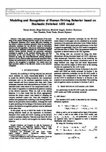
u1 , u2 u4 Fig. 1

Definition of the input signals.

Throughout this paper, we focus on the driving behavior on the expressway which consists of ‘following the leading vehicle’, ‘lane changing’, ‘overtaking’, and so on. All driving data are obtained by using Driving Simulator (DS) [19]. The view from the driver is shown in Fig.2. The driver input, i.e., the sensory information of the driver is defined as follows (Fig.1): • Range from the leading car: u1 • Range rate between the leading and examinee’s cars: u2 • Lateral displacement from the leading car: u3 • Yawing angle of examinee’s car: u4 • Index for approaching (KdB): u5 • Amount of time duration that the examinee looks at the left side mirror in the latest 10 [s] (TL): u6 • Amount of time duration that the examinee looks at the right side mirror in the latest 10 [s] (TR): u7 u6 and u7 are obtained by using the ‘eyemark recorder’ developed by nac image technology Inc. KdB is an index which represents the logarithm of a time derivative of the area of the back of the leading car projected on the driver’s retina [20]. In [20], it is verified that this index plays an important role in the recognition of approaching objects from viewpoint of the cognitive science. Although it is unlikely that the KdB is able to be measured directly, it can be calculated using u1 and u2 by following equation.  1 −10 × log(| − 2 × uu23 × 5×10 −8 |)   1  if u2 > 0 (1) KdB = 1 10 × log(| − 2 × uu23 × 5×10  −8 |)  1  if u2 < 0

Fig. 2

View from the driver.

The large KdB implies that the driver is facing dangerous situation. Also, the driver output is defined as follows: • Steering angle: y1 • Pedal operation: y2 These input and output variables are chosen so that the resulting model can express the behavioral characteristics underlying the observed data. Furthermore, these variables can be observed in the real driving situation by using existing sensors. Based on these input and output definitions, the mathematical model of the driving behavior is discussed in the next subsection. 2.2 PWARX model as mathematical representation of multi-mode driving behavior In this subsection, the PWARX model is introduced as a mathematical model of the driving behavior. The PWARX model consists of several ARX models, i.e., modes, and can express a complex input-output relationship with any approximation level by appropriately controlling the number of modes. We consider the following first order PWARX model which has s modes: y(k) = f (r(k)) + ²(k)  θ1 r(k) if r(k) ∈ R1     θ2 r(k) if r(k) ∈ R2 f (r(k)) = ..  .    θs r(k) if r(k) ∈ Rs

(2)

where ²(k) is an equation error. y(k) and r(k) are also defined as follows: y(k) = (y1 (k) y2 (k))T (3) r(k) = (u1 (k − 1) u2 (k − 1) · · · u7 (k − 1) y1 (k − 1) y2 (k − 1))T (4) The subscript k denotes the sampling index (k = 1, 2 . . . , n). Furthermore, θi (i = 1, · · · , s) is a (2 × 9) unknown matrix to be identified from the data, and is supposed to have a form:

µ θi =

T θi,1 T θi,2

¶ (5)

In the PWARX model, not only parameters θi but also the partitions of the subspaces R1 , · · · , Rs are unknown. Therefore, it is not straightforward to assign each observation (y(k), r(k)) at sampling instant k to the corresponding mode. To resolve this problem, a clustering based technique is developed in [12] under the definition of interesting feature vector which represents the local dynamical characteristics underlying (y(k), r(k)). In the next subsection, this feature vector is introduced. 2.3

Definition of feature vector

1. Assume that the set of sample data {(y(j), r(j))}, (j = 1, 2 . . . , n) is given. For each sample data (y(j), r(j)), collect the neighboring c data in the (y, r) space, generate the local data set LDj , and calculate the feature vector ξj (see Fig.3(a)). Note that the index j indicates the order not in the time space but in the data space. The feature vector ξj consists of the local parameters LD T LD T T ((θj,1 ) , (θj,2 ) ) in the local ARX model for the LDj and the mean value mj of the data r in the LD T ) (l = 1, 2) and mj are calculated as LDj . (θj,l follows: LD θj,l = (ΦTj Φj )−1 ΦTj yLDj ,l 1 X mj = r c

(6) (7)

r∈LDj

where yLDj ,l (c × 1; l = 1, 2) is the output samples in the LDj , and Φj is given by Φj = (r1 r2 · · · rc )T (r ∈ LDj ).

where SSRj,l (ΦT Φj )−1 c − (9 + 1) j

(10)

T SSRj,l = yLD (I − Φj (ΦTj Φj )−1 ΦTj )yLDj ,l j ,l

Qj =

X

2.4 Unsupervised hierarchical clustering The unsupervised hierarchical clustering is applied to the feature vectors ξj (j = 1, · · · , n). The clustering algorithm is listed below: 1. Regard each feature vector ξj as each cluster Cj , i.e., each cluster consists only of one feature vector. Calculate the dissimilarity Dp,q between any two clusters Cp and Cq by using the following dissimilarity measure: Dp,q = k ξp − ξq k2R−1

p,q

−1 = (ξp − ξq )T Rp,q (ξp − ξq )

(11) T

(r − mj )(r − mj )

(12)

r∈LDj

The feature vector ξj represents the combination of the local dynamics and data. By this definition, the data is classified based not only on the value of data but also

(13)

where −1 Rp,q = Rp−1 + Rq−1 .

(14)

2. Unify two clusters Cx and Cy which shows the smallest Dx,y . The unified cluster is denoted by Cr . If all clusters are unified, terminate the algorithm. Otherwise, go to step 3. 3. Calculate the dissimilarity Dr,t between Cr and Ct for all t (t 6= r) by using the following dissimilarity measure: X X nr n t k ξir −ξit k2R−1 (15) Dr,t = ir ,it nr + nt ξir ∈Cr ξit ∈Ct

where nr and nt are numbers of feature vectors belonging to clusters Cr and Ct , respectively. Go to step 2.

(8)

LD T LD T As the result, ξj = ((θj,1 ) , (θj,2 ) , mTj )T . 2. For each feature vector ξj , the following covariance matrix Rj is calculated:   Vj,1 0 0 Vj,2 0  Rj =  0 (9) 0 0 Qj

Vj,l =

on the similarity of the underlying dynamics. Furthermore, the covariance matrix Rj represents the confidence level of the corresponding feature vector ξj . Rj is used as the weighting matrix in the calculation of the dissimilarity between feature vectors in the clustering procedure.

After this clustering procedure, the classification of the feature vector space is achieved together with a dendrogram which shows the hierarchical classification for different number of modes. Since the transformation from the feature vector (ξ) space to the original observed data (y, r) space is straightforward, the mode segmentation of the observed data is obtained together with the hierarchical structure. Note that once mode segmentation of the data is achieved, the identification of the parameters θi and the partitions of the subspaces R1 , · · · , Rs in the PWARX model (2) is straightforward. 3.

Analysis of driving behavioral data

3.1 Driving environment In this paper, the following driving environment on

y

each examinee can drive as his/her usual manner. j

Parameters jLD Mean value mj

3.2 Observed behavioral data and clustering results

LDj Transform to feature space (y(j),r(j))

3

u (b) Feature space

Unsupervised clustering

y

Transform to data space

Fig. 3

s=2

2 1.5

1

u (b) Feature space (clustered)

4

2.5

Dissimilarity

(a) Data space

x 10

s=5

0.5

(d) Data space (clustered)

0

Outline of mode segmentation.

Data Fig. 4

the expressway was designed on the driving simulator which provides a stereoscopic immersive vision. • The expressway is endless, and has two lanes, the cruising lane and the passing lane. • There are 10 cars on the cruising lane. Five of them are running ahead of the examinee’s car. The remaining five cars are running behind the examinee’s car. Their velocities vary from 70 to 85[km/h]. Once the examinee’s car overtakes the leading car, then the tale-end car on the cruising lane is moved to the head of the cars running on the cruising lane. The examinee is not aware of this change. • There are 10 cars on the passing lane. Five of them are running ahead of the examinee’s car. The remaining five cars are running behind the examinee’s car. Their velocities vary from 90 to 110[km/h]. Once the examinee’s car is overtaken by the car on the passing lane, then the top car on the passing lane is moved to the tale-end of the cars running on the passing lane. The examinee is not aware of this change. • The range between cars is set to be 50 to 300[m], and there is no collision between cars except the examinee’s car. • There is no lane change of the cars except the examinee’s car. Under this driving environment, five examinees performed the test driving. Note that the examinees were provided with the instruction ‘Drive the car according to your usual driving manner’. Since this instruction is ‘loose’ instruction, the examinees do not concern much about the environmental information. As the result,

Dendrogram of clustering (Examinee A).

The unsupervised clustering based on the feature vector shown in the previous section has been applied to the observed driving behavioral data. The dendrogram obtained from the proposed strategy is shown in Fig.4. In Fig.4, the vertical axis represents the dissimilarity between clusters. When the two clusters are unified, the corresponding dissimilarity is designated by the horizontal bar. The horizontal axis represents the data which is rearranged after the clustering to show the hierarchical structure clearly. From this figure, we can clearly understand the hierarchical structure in the driving behavior. As the typical example, the two dashed horizontal lines are superimposed. The upper line shows the case that the number of modes (clusters) s, i.e., the number of the ARX models in (2) is set to be two. On the other hand, the lower line shows the case that s is set to be five. In Fig.5, the observed driving (input-output) profiles are shown. All profiles are normalized before clustering. In the profile of the lateral displacement, it takes positive value when the examinee’s vehicle is on the right side of the leading car. The steering angle takes positive value when the examinee turns it clockwise. Also, the pedal operation takes positive value when the accelerator is stepped on, and takes negative value when the braking pedal is stepped on. Note that the range, the rage rate and the lateral displacement profiles show discontinuity at some time instants. Since these variables are defined by the relative displacement from the leading car, if the examinee’s car changes the driving lane, these variables change discontinuously. In addition, the clustering results in the case of two-mode modeling are indicated by colors in Fig.5.

1 Range

Range

1 0.5

RangeRate

0

1 0 −1

Lateral

1

Lateral

0

0

Yaw

Yaw

1

0

0

−1

−1

1

1

KdB

0

1

0.5 0

1 TR

1

0.5 0

1

1

Steering

0

0 −1

0 300

400

500 Time[s]

600

700

800

Fig. 5 Observed profiles and mode segmentation result (Examinee A, 2modes).

Thus, the mode segmentation works well. In order to investigate the behavioral meaning of each mode, a part of the profile of the lateral displacement is enlarged in Fig.7. As shown in Fig.7, the meaning of two modes can be understood as the ‘Following on Cruising Lane + Passing’ (Mode 1: FC+P mode) and ‘Following on Passing Lane + Returning’ (Mode 2: FP+R mode), respectively. Note that the range rate is always positive in the Mode 2 in Fig.5. This implies that there exist some implicit common sense in the driving behavior such as ‘should keep the legal speed on the passing lane’ in addition to the instruction. Thus, the symbolization of the behavior can be achieved based on the ‘dissimilarity’ of the underlying dynamics. No prior knowledge is necessary in this symbolization except the definition of the input and output variables of the behavior.

200

300

400

500 Time[s]

600

700

800

Fig. 6 Observed profiles and mode segmentation result (Examinee A, 5modes).

M ode 1

Later al

200

0 −1

1 0 -1

260

280

M ode 2

300 Time[s]

320

340

Fig. 7 Enlarged profile of the lateral displacement (Examinee A, 2modes).

Mode 1

Lateral

−1

0 −1 1

Pedal

1 Pedal

0.5 0

0.5

3.3

0 −1

TL

TL

1

1

1

TR

0 −1

−1

−1

Steering

1

−1

KdB

RangeRate

0

0.5

1 0 -1

260

Mode 2

280

Mode 3

300 Time[s]

Mode 4

320

Mode 5

340

Fig. 8 Enlarged profile of the lateral displacement (Examinee A, 5modes).

Discussion

In order to analyze the hierarchical structure of the behavior, the clustering results in the case of five-mode modeling are shown in Fig.6, and the enlarged lateral

displacement is shown in Fig.8. From Fig.8, we can see that the two-mode model is further decomposed into the local behaviors; they are ‘Long Range Following on Cruising Lane’ (Mode 1: LRFC mode), ‘Short Range

Following on Cruising Lane’ (Mode 2: SRFC mode), ‘Passing’ (Mode 3: P mode), ‘Following on Passing Lane’ (Mode 4: FP mode), and ‘Returning’ (Mode 5: R mode). The switching between these modes corresponds to the change of the control modes caused by either the driver’s intention or change of the environment. The hierarchical relationship between these modes found in the dendrogram is depicted in Fig.9. Thus, the hierarchical structure of the driving behavior can be obtained in a quite consistent manner. One of the significant contributions of this work is that this hierarchical structure is obtained automatically based only on the observation (including the definition of the input and output signals) and data processing from viewpoint of the dynamics. Since this hierarchy clearly expresses the multiple abstraction level of the human behavior, the proposed framework is expected to be a basis for the design of many human centric systems.

2 Mode

Following on Cruising Lane + Passing Mode

Following on Passing Lane + Returning Mode

5 Mode Long Range Following on Cruising Lane Mode

Short Range Following on Cruising Lane Mode

Passing Mode

Following on Passing Lane Mode

Returning Mode

Fig. 9 Identified hierarchical structure of driving behavior (Examinee A).

4.

Development of symbolic behavior model and its application to behavior prediction

In this section, the human behavior is considered as a source which is capable of generating a specific language (set of symbol strings). This can be realized by regarding the driving mode estimated in the section 3 as a symbol. The grammar G of the language is the set of production rules that specifies all the strings in the language and their relationships. Once the grammar is found, the grammar itself is a model for the source of the behavior. 4.1

Definition of behavioral grammar

First of all, the behavioral grammar G is defined as follows: G = {Σm , Σe , S, P }

(16)

Σm is a mode alphabet, i.e., the set of mode symbols defined by the clustering introduced in section 3. Therefore, the number of mode symbols |Σm | = s, i.e., the

number of ARX models. Σe is an environment alphabet, i.e., the set of symbols created by a vector quantization of the environmental information. The number of environment symbols |Σe | depends on the quantization. In the proposed framework, Σm and Σe are regarded as a terminal alphabet and a nonterminal alphabet in the standard grammar, respectively. S is a special nonterminal symbol used to start the generation of string. P is a set of production rules, i.e., the substitution rules (denoted by a → b) used to generate the strings. The n − type production rules are defined as substitution rules of the form mk−n · · · mk−1 Ek → mk−n · · · mk−1 mk δ

(17)

where mk−n · · · mk−1 is a sequence of mode symbols, Ek is an environment symbol, and δ is a special nonterminal symbol. δ is used to indicate the conclusion, or not, of a generated string by the use of the following special set of production rules: ½ δ → Ek+1 or (18) δ→λ where λ denotes the empty symbol. The n − type production rule encodes the evolution of the mode depending on its n past modes and on the environment symbol E. Therefore, the n − type production rule can be regarded as a symbolic dynamics whose order is specified by n. Once G is identified, the symbolic behavior can be computed by executing the production rules. 4.2

Grammatical inference

Development of the symbolic behavior model can be formulated as the grammatical inference problem [22] under the suitable definitions of the mode and environment alphabets. Grammatical inference, in general, is the identification of a grammar from a set of examples. The main part of the grammatical inference is the generation of the production rules based on the observation, and is realized by the following procedure (See [22] for detail). 1. A 0 − type production rule is assumed for every newly occurring environment symbol. 2. A new (n + 1) − type production rule is generated whenever the data conflicts with the previously established n − type production rules. The conflicting n − type production rules are also promoted to (n + 1) − type production rules or are deleted if there is not sufficient information in the past. As an example, consider the following symbol sequence which is supposed to be obtained from the observation: Time t1 t2 t3 t4 Env. symbol OA OB O A OA Mode symbol e d c b mi ∈ {b, c, d, e}, Ei ∈ {OA , OB }

t5 OB d

t6 OA e

At the beginning, the algorithm analyzes the leading symbols. Since no other information is yet available, a 0 − type production rule OA → eδ is assumed. After analyzing the second symbol, the algorithm establishes another 0 − type production rule OB → dδ. The third symbol would yield a 0 − type production rule OA → cδ. However, this production rule contradicts the previously established OA → eδ. Therefore, in this case, a 1 − type production rule dOA → dcδ is obtained. The 0 − type production rule OA → eδ is deleted because no information is available in the past on the first symbol ‘e’. At the next step, we obtain the production rule cOA → cbδ. Another conflict arises when we reach the last symbol. Then a 2 − type production rule bdOA → bdeδ is obtained and dOA → dcδ is revised to edOA → edcδ. As the result, the following production rules are generated: OB → dδ, bdOA → bdeδ, 4.3

cOA → cbδ, edOA → edcδ

(19)

Application to symbolic behavior modeling and prediction

Table 1

Representative value of each environment symbol

variable L[m] X1 [m] X2 [m] X3 [m] X4 [m] X5 [m] X6 [m] V1 [km/h] V2 [km/h] V3 [km/h] V4 [km/h] V5 [km/h] V6 [km/h]

OA 3.51 225.43 99.85 -163.60 118.21 -52.40 -246.93 -27.71 -27.43 -27.40 21.02 18.28 19.93

OB 2.23 618.01 354.52 -119.79 204.18 -40.03 -180.44 -26.40 -27.01 -35.22 13.19 4.57 9.76

OC 0.44 267.23 118.24 -72.30 141.11 -60.75 -258.79 -28.88 -29.12 -28.89 18.54 7.40 15.82

OD 0.48 258.12 72.98 -31.16 203.39 -38.78 -226.72 -16.38 -15.37 -15.30 35.25 1.82 30.37

OE 3.49 360.29 116.02 -487.75 93.06 -61.01 -259.18 -29.18 -26.59 -35.08 11.25 11.29 11.41

variable L[m] X1 [m] X2 [m] X3 [m] X4 [m] X5 [m] X6 [m] V1 [km/h] V2 [km/h] V3 [km/h] V4 [km/h] V5 [km/h] V6 [km/h]

OF 3.54 163.20 52.25 -65.00 104.10 -96.38 -300.58 -13.32 -12.14 -8.79 39.27 33.51 38.85

OG 3.00 255.99 26.28 -135.92 67.83 -114.85 -334.29 1.83 -0.57 0.52 50.85 47.61 50.97

OH 0.40 302.79 78.48 -21.02 122.16 -71.96 -305.18 -12.15 -13.52 -11.37 38.02 30.85 38.12

OI 3.69 427.63 193.21 -158.32 113.27 -77.15 -245.84 -13.31 -13.77 -19.18 29.67 26.04 27.75

OJ 0.64 128.47 10.30 -208.27 99.87 -104.00 -350.50 -11.21 -10.44 -8.34 38.40 34.99 38.52

4.3.1 Definition of environment symbol First of all, the environment symbols are defined by the vector quantization of the relative position (Xi ) and relative velocity (Vi ) of the six surrounding cars as shown in Fig.10. Since the goal is to realize the long-term prediction based on the symbolic model, the wider range of cars are considered as the environment than the definition of the input variables for the PWARX model. The CSL (Competitive and Selective Learning) algo-

Passing Lane

Examinee’s Car

3

Cruising Lane

6

2

5

Fig. 10

1

case of the five-mode model. The obtained rules are classified into two kinds of rules: (1) the rule to keep the same mode, (2) the rule to change the mode. In Fig.11, the symbols a, b, c, d and e correspond to the driving modes 1, 2, 3, 4 and 5 in section 3.3, respectively. For example, ej bk OF → c implies that the driving mode ‘e’ (Mode5: returning) continues j times followed by the driving mode ‘b’ (Mode2: short range following in the cruising lane) which also continues k times in the past, and the current environment symbol is ‘OF ’, then the next mode is changed to the driving mode ‘c’ (Mode3: passing).

4

Definition of environment.

rithm [21] was used for the quantization. The necessary number of symbols depends on the complexity of the environment. Here, 10 symbols (OA to OJ ) were obtained and their representative values are shown in Table 1. 4.3.2 Behavior prediction based on production rules By applying the grammatical inference to the two-mode model and the five-mode model, we have developed the two symbolic behavior models with different definition of the mode symbol. The example of the generated rules for the examinee A is depicted in Fig.11 in the

anOI

a

bmOA

d lOA

e

e jbkOF

b …..

c …..

a, b, c, d, e: driving mode n, m, l, j, k : number of continuation Fig. 11 model).

Example of the generated production rules (five-mode

The number of identified rules and the average of rule type are shown in Table 2. In the two-mode model, the number of identified rules is smaller, but the average of rule type is higher compared with the five-mode

model. This implies that these factors depend on the ‘resolution’ of the symbolic representation. Another interesting inquiry is that the number of identified rules varies from examinee to examinee. The examinee who has great number of rules (like the examinee E) can be considered to have an inconsistent driving manner. In addition, the prediction of the behavior based on the symbolic model was performed. In order to predict the future behavior, the prediction of the environment symbol must be considered. In this work, the prediction of the environment symbol was realized by a simple first-order prediction of Xi s and Vi s. Figure 12 shows the success rate of the prediction for various prediction horizon using the several models with different number of modes (1 step is 240 [ms]). From Fig.12, the success rate goes down as the prediction horizon becomes longer. However, even in the five-mode model, about 70% success rate is achieved for 10step (2.4[s]) ahead prediction. Furthermore, the low-mode model shows higher success rate than the high-mode model. Thus, the proposed framework can control the prediction accuracy by choosing the ‘resolution’ of the symbolic representation. Table 2 nees)

Statistics of generated production rules (five examitwo-mode model Number Ave. of of rules rule type

five-mode model Number Ave. of of rules rule type

Exam.

Number of data

A

2851

90

27.6

1026

18.4

B

2908

120

22.6

996

17.7

C

2424

273

21.0

962

18.2

D

3008

448

21.0

1251

18.4

E

3063

670

20.6

1640

14.8

Success rate [%]

100 80 60

2 mode model 3 mode model 4 mode model 5 mode model

40 20 0 1

2

3

4

5

6

7

8

9

10

Prediction horizon Fig. 12 Success rate of the prediction for various prediction horizon (all examinees).

5.

Conclusion

This paper has presented a new hierarchical mode

segmentation of the observed driving behavioral data based on the multi-level abstraction of the underlying dynamics. By synthesizing the ideas of the feature vector definition revealing the dynamical characteristics and the unsupervised clustering technique, the hierarchical mode segmentation has been achieved. The identified mode can be regarded as a kind of symbol in the abstract model of the behavior. Second, the grammatical inference technique was introduced to develop the context-dependent grammar of the behavior, i.e., the symbolic dynamics of the human behavior. In addition, the behavior prediction based on the obtained symbolic model was performed and discussed. The proposed framework enables us to make a bridge between the signal space and the symbolic space in the understanding of the human behavior. The design of the environment symbol with hierarchical structure and application to anomaly detection to realize the safety man-machine systems are our future works. Acknowledgments This work was supported by Grant-in-Aid for Scientific Research (KAKENHI 21650070) and Strategic Information and Communications R&D Promotion Program (SCOPE 082006002) Japan. References [1] D.McRuer and D.Weir: Theory of manual vehicular control, Ergonomics, Vol.12, pp.599-633, 1969. [2] C.MacAdam: Application of an optimal preview control for simulation of closed-loop automobile driving, IEEE Trans. on Syst. Man and Cyber., Vol.11, No.9, pp.393-399, 1981. [3] A.Modjtahedzadeh and R.Hess: A Model of Driver Steering Control Behavior for Use in Assessing Vehicle Handling Qualities, ASME J. of Dynam. Syst. Meas. Contr., Vol.15, Sept., pp.456-464, 1993. [4] T.Pilutti and A.G.Ulsoy: Identification of Driver State for Lane-Keeping Tasks, IEEE Trans. on Syst. Man and Cyber., Part A, Vol.29, No.5, pp.486-502, 1999. [5] J.Sjoberg, Q.Zhang, L.Ljung, A.Benveniste, B.Deylon, P.Y. Glorenner, H.Hjalmarsson, and A. Juditsky: Nonlinear Black-Box Modeling in System Identification: a Unified Overview, Automatica, vol.31, no.12, pp.1691-1724, 1995. [6] K.S.Narendra and K.Pathasarathy: Identification and Control of Dynamical Systems Using Neural Networks, IEEE Trans. on Neural Networks, vol.1, no.1, pp.4-27, 1990. [7] M.C.Nechyba, Y.Xu: Human Control Strategy: Abstraction, Verification, and Replication, IEEE Control Systems Magazine, October pp.48-61, 1997. [8] W.Takano, A.Matsushita, K.Iwao and Y.Nakamura: Recognition of Human Driving Behaviors based on Stochastic Symbolization of Time Series Signal, Proc. of IEEE/RSJ Int. Conf. on Intelligent Robots and Systems, pp.167-172, 2008. [9] F.A.Mussa-Ivaldi, S.F.Giszter, E.BIzzi: Linear combinations of primitives in vertebrate motor control, Proc. of the National Academy of Science, 91, pp.7534-7538, 1994. [10] C.Bregler, J.Malik: Learning and recognizing human dynamics in video sequences, Proc.of IEEE Conf. on Computer Vision and Pattern Recognition, pp.568-674, 1997.

[11] D.D.Vecchio, R.M.Murray, P.Perona: Decomposition of human motion into dynamics-based primitives with application to drawing tasks, Automatica Vol. 39, pp.2085-2098, 2003. [12] G.Ferrari-Trecate, M. Muselli, D. Liberati, M. Morari: A clustering technique for the identification of piecewise affine system, Automatica,Vol.39, pp.205-217, 2003. [13] T.Roll, A.Bemporad, L.Ljung: Identification of piecewise affine systems via mixed-integer programming, Automatica, Vol.40, pp.37-50, 2004. [14] A. Lj. Juloski, S. Weiland, W. P. M. H. Heemels: A Bayesian Approach to Identification of Hybrid Systems, IEEE Trans. on Automatic Control, Vol. 50, No. 10, pp.1520-1533, 2005. [15] R.Vidal, S.Soatto, Y.Ma and S.Sastry: An Algebraic Geometric Approach to the Identification of a Class of Linear Hybrid Systems, Proc. of IEEE Conf. on Decision and Control, pp.167-172, 2003. [16] B.S.Everitt: Cluster Analysis, Edward Arnold, 4th edition, 2001. [17] J.H.Kim, S.Hayakawa, T.Suzuki, K.Hayashi, S.Okuma, N.Tsuchida, M.Shimizu, S.Kido: Modeling of Driver’s Collision Avoidance Maneuver based on Controller Switching Model, IEEE Trans. on System, Man and Cybernetics, part B, Vol.35, No.6, pp.1131-1143, 2005. [18] S.Sekizawa, S.Inagaki, T.Suzuki, S.Hayakawa, N.Tsuchida, T.Tsuda, H.Fujinami: Modeling and Recognition of Driving Behavior Based on Stochastic Switched ARX Model, IEEE Trans. on Intelligent Transportation Systems, Vol. 8, NO. 4, pp.593-606, 2007. [19] T.Akita, T.Suzuki, S.Hayakawa, S.Inagaki: Analysis and Synthesis of Driving Behavior based on Mode Segmentation, Proc. of Int. Conf. on Control, Automation and Systems, pp.2884-2889, 2008. [20] T.Wada, S.Doi, K.Imai, N.Tsuru, K.Isaji, H.Kaneko: Analysis of Drivers’ Behaviors in Car Following Based on a Performance Index for Approach and Alienation, Proc. of SAE2007 World Congress, SAE paper 2007-01-0440. [21] N.Ueda, R.Nakano: A New Competitive Learning Approach Based on an Equidistortion Principle for Designing Optimal Vector Quantizers, Neural Networks, Vol.7, No.8, pp.1211–1227, 1994. [22] K.S.Fu, T.L.Booth: Grammatical Inference: Introduction and Survey - Part II, IEEE Trans. on System, Man and Cybernetics, Vol.5, pp.409-423, 1975.

Hiroyuki Okuda was born in Gifu, JAPAN, in 1982. He received the B.E. and M.E. degrees in Advanced Science and Technology from Toyota Technological Institute, JAPAN in 2005 and 2007, respectively. He is a doctoral student at the Department of Mechanical Science and Engineering of Nagoya University, JAPAN. His research interests are in the areas of system identification of hybrid dynamical system and its application to modeling of human behavior, design of human centered mechatronics and biological signal processing. Mr.Okuda is a member of the IEEJ and SICE.

Tatsuya Suzuki was born in Aichi, JAPAN, in 1964. He received the B.E., M.E. and PhD degrees in Electronic Mechanical Engineering Department from Nagoya University, JAPAN in 1986, 1988 and 1991, respectively. From 1998 to 1999, he was a visiting researcher of the Mechanical Engineering Department of U.C.Berkeley. Currently, he is a professor of the Department of Mechanical Science and Engineering of Nagoya University. He won the outstanding paper award in ICCAS 2008. He also won the journal paper awards from IEEJ and SICE in 1995 and 2009, respectively. His current research interests are in the areas of modeling and analysis of hybrid dynamical systems, and design of human centered mechatronics. Dr.Suzuki is a member of the IEEJ, SICE, ISCIE, RSJ, JSME and IEEE.

Ato Nakano was born in Shizuoka, JAPAN, in 1984. He received the B.E. and M.E. degrees in Mechanical Science and Engineering Department from Nagoya University, JAPAN in 2007 and 2009, respectively. He is currently working at Toyota Motor Corporation.

Shinkichi Inagaki was born in Mie, JAPAN, in 1975. He received the PhD degree in Precision Engineering from Tokyo University, JAPAN in 2003. From 2003 to 2008, he had been a Research Associate at Nagoya University, JAPAN. Since 2008, he has been an Assistant Professor at Nagoya University. His research interests are in the area of autonomous decentralized systems, robotics and manmachine cooperative systems. Dr.Inagaki is a member of the IEEE, SICE, RSJ and JSME.

Soichiro Hayakawa was born in Aichi, JAPAN, in 1968. He received the Ph.D. degree in Electrical and Electronic Engineering from Nagoya University, Nagoya, Japan, in 1996. From 1996 to 2009, he has been an assistant professor with Toyota Technological Institute. Currently, he is a associate professor of the Department of Mechanical Engineering of Mie University. His current research interests are in the areas of modeling and analysis of human behavior based on hybrid dynamical systems for man-machine cooperative system. Dr.Hayakawa is a member of the IEEJ, IEICE, SICE and RSJ.