Keywords: Interstitial Lung Disease Detection, Convolutional Neural Network, .... truth annotation. The L2 cost function to be minimized is defined as. L(yi, yi) = ..... Gong, Y., Wang, L., Guo, R., Lazebnik, S.: Multi-scale orderless pooling of deep ...
Multi-label Deep Regression and Unordered Pooling for Holistic Interstitial Lung Disease Detection Mingchen Gao, Ziyue Xu, Le Lu, Adam P. Harrison, Ronald M. Summers, and Daniel J. Mollura Department of Radiology and Imaging Sciences, National Institutes of Health (NIH), Bethesda, MD 20892
Abstract. Holistically detecting interstitial lung diseases (ILDs) from CT images is challenging yet clinically important. Unfortunately, most existing solutions rely on manually provided regions of interest, limiting their clinical usefulness. In addition, no work has yet focused on predicting more than one ILD from the same CT slice, despite the frequency of such occurrences. To address these limitations, we propose two variations of multi-label deep convolutional neural networks (CNNs). The first uses a deep CNN to detect the presence of multiple ILDs using a regression-based loss function. Our second variant further improves performance, using spatially invariant Fisher Vector encoding of the CNN feature activations. We test our algorithms on a dataset of 533 patients using five-fold cross-validation, achieving high area-under-curve (AUC) scores of 0.982, 0.972, 0.893 and 0.993 for Ground Glass, Reticular, Honeycomb and Emphysema, respectively. As such, our work represents an important step forward in providing clinically effective ILD detection. Keywords: Interstitial Lung Disease Detection, Convolutional Neural Network, Multi-label Deep Regression, Unordered Pooling, Fisher Vector Encoding
1
Introduction
Interstitial lung disease (ILD) refers to a group of more than 150 chronic lung diseases that causes progressive scarring of lung tissues and eventually impairs breathing. The gold standard imaging modality for diagnosing ILD is high resolution computed tomography (HRCT) [1, 2]. Fig. 1 depicts examples of the most typical ILDs. Automatically detecting ILD from HRCT images would help the diagnosis and treatment of this morbidity. The majority of previous work on ILD detection is limited to patch-level classification, which classifies small patches from manually generated regions of interest (ROIs), into one of the ILDs. Approaches include restricted Boltzmann machines [3], convolutional neural networks (CNNs) [4], local binary patterns [5, 6] and multiple instance learning [7]. An exception to the patch-based approach is the recent work of Gao et al. [8], which investigated a clinically more realistic scenario for ILD classification, assigning a single ILD label to any holistic two-dimensional axial CT slice This research is supported by NIH intramural research program, Center for Infectious Disease Imaging (CIDI), Imaging Biomarkers and Computer-Aided Diagnosis Laboratory. Acknowledgment to Nvidia Corp. for donation of K40 GPUs.
without any pre-processing or segmentation. Although holistic detection is more clinically desirable, the underlying problem is much harder without knowing the ILD locations and regions a priori. The difficulties lie on several aspects, which include the tremendous amount of variation in disease appearance, location, and configuration and also the expense required to obtain delicate pixel-level ILD annotations of large datasets for training. Despite of its importance, this challenge of detecting multiple ILDs simultaneously without the locations has not been addressed by previous studies [3, 4, 8, 9], including that of Gao et al. [8], which all treat ILD detection as a single-label classification problem. When analyzing the Lung Tissue Research Consortium (LTRC) dataset [2], the most comprehensive lung disease image database with detailed annotated segmentation masks, we found that there are significant amounts of CT images associated with two or more ILD labels. For this reason, and partially inspired by the recent natural image classification work [10], we model the problem as multi-label regression and solve it using a CNN. We employ the deep CNN regression model because of its simplicity and the fact that deep image features and final cost functions can be seamlessly learned [11, 12]. We note that multi-label regression has also been used outside of ILD contexts for heart chamber volume estimation [13, 14]. However, this prior work used hand-crafted features and random-forest based regression, whereas we employ learned CNN-based features, which have enjoyed dramatic success in recent years over hand-crafted variants [11]. Thus, unlike prior ILD detection work [3–6, 8], our goal is to detect multiple ILDs on holistic CT slices simultaneously, providing a more clinically useful tool. While CNNs are a powerful tool, their feature learning strategy is not invariant to the spatial locations of objects or textures within a scene. This order-sensitive feature encoding, reflecting the spatial layout of the local image descriptors, is effective in object and scene recognition. However, it may not be beneficial or even be counter-productive for texture classification [15]. The spatial encoding of order-sensitive image descriptors can be discarded via unordered feature encoders such as Bag of Visual Words (BoVW), Fisher Vectors (FV) [16], or aggregated by order-sensitive spatial pyramid matching (SPM). Given the above considerations, we enhance our CNN-regression approach using spatialinvariant encodings of feature activations for multi-label multi-class ILD detection. Thus, in this work, we propose two variations of multi-label deep convolutional neural network regression (MLCNN-R) models to address the aforementioned challenges. First, an end-to-end CNN network is trained for multi-label image regression. The loss functions are minimized to estimate the actual pixel numbers occupied per ILD class or the binary [0,1] occurring status. Second, the convolutional activation feature maps at different network depths are spatially aggregated and encoded through FV [16] method. This encoding removes the spatial configurations of the convolutional activations and turns them into location-invariant representations. This type of CNN is also referred as FVCNN [15]. The unordered features are then trained using a mutlivariate linear regressor (Mvregress function in Matlab) to regress the numbers of ILD pixels or binary labels. Our proposed algorithm is demonstrated using the LTRC ILD dataset [2], composed of 533 patients. Our experiments use five-fold cross-validation (CV) to detect the most common ILD classes of Ground Glass, Reticular, Honeycomb and Emphysema. Experimental results demonstrate the success of our approach in tackling the challenging problem of multi-label multi-class ILD classification.
Fig. 1. Examples of ILD patterns. Every voxel in the lung region is labeled as healthy or one of the four ILD diseases: Ground Glass, Reticular, Honeycomb or Emphysema. The first row is the lung CT images. The second row is their corresponding labeling.
2
Methods
Our algorithm contains two major components: 1) we present a squared L2 loss function based multi-label deep CNN regression method to estimate either the observable ILD areas (in the numbers of pixels), or the binary [0,1] status of “non-appearing” or “appearing”. This regression-based approach allows our algorithm to naturally preserve the co-occurrence property of ILDs in CT imaging. 2) CNN activation vectors are extracted from convolutional layers at different depths of the network and integrated using a Fisher Vector feature encoding scheme in a spatially unordered manner, allowing us to achieve a location-invariant deep texture description. ILD classes are then discriminated using multivariate linear regression. 2.1
CNN Architecture for Multi-label ILD Regression
Deep CNN regression is used to calculate the presence or the area of spatial occupancy for IDL in the image, where multiple pathology patterns can co-exist. The squared L2 loss function is adopted for regression [10] instead of the more widely used softmax or logistic-regression loss for CNN-based classification [4, 8, 11]. There are multiple ways to model the regression labels for each image. One straightforward scheme is to count the total number of pixels annotated per disease to represent its severity, e.g., Fig. 2 left. We can also use a step function to represent the presence or absence of the disease, as shown in Fig. 2 middle, where the stage threshold T may be defined using clinical knowledge. For any ILD in an image, if its pixel number is larger than T , the label is set to be 1; otherwise as 0. A more sophisticated model would have a piecewise linear transform function, mapping the pixel numbers towards the range of [0,1] (Fig.2 right). We test all approaches in our experiments. Suppose that there are N images and total c types of ILD diseases to be detected or classified, the label vector of the ith image is represented as a c-length multivariate vector yi = [yi1 , yi2 , ..., yic ]. An all-zero labeling vector indicates that the slice is healthy or has
no targeted ILD disease found based on the ground truth annotation. The L2 cost function to be minimized is defined as L(yi , y ˆi ) =
N X c X
(yik − yˆik )2 ,
(1)
i=1 k=1
There are several successful CNN structures from previous work, such as AlexNet [11], VGGNet [17] . We employ a variation of AlexNet, called CNN-F [18], for a trade-off between efficiency and performance based on the amount of available annotated image data. CNN-F contains five convolutional layers, followed by two fully-connected (FC) layers. We set the last layer to the squared L2 loss function. Four classes of ILD diseases are investigated in our experiments: Ground Glass, Recticular, Honeycomb and Emphysema (other classes have too few examples in LTRC database [2]). The length of yi is c = 4 to represent these four ILD classes. Based on our experience, random initialization of the CNN parameters worked better than ImageNet pre-trained models. Model parameters were optimized using stochastic gradient descent.
Fig. 2. Three functions for mapping the number of pixels to the regression label.
2.2
Unordered Pooling Regression via Fisher Vector Encoding
In addition to CNN-based regression, we also test spatially invariant encoding of CNN feature activations. We treat the output of each k-th convolutional layer as a 3D descriptor field Xk ∈ RWk ×Hk ×Dk , where Wk and Hk are the width and height of the field and Dk is the number of feature channels. Therefore, the whole deep feature activation map is represented by Wk × Hk feature vectors and each feature vector is Dk dimension. We then invoke FV encoding [16] to remove the spatial configurations of total Wk × Hk vectors per activation map. Following [16], each descriptor xi ∈ Xk is soft-quantized T using a Gaussian Mixture Model. The first- and second-order differences (uTi,m , vi,m ) between any descriptor xi and each of the Gaussian cluster mean vectors {µm }, m = 1, 2, ..., M are accumulated in a 2M Dk -dimensional image representation: T T , ..., uTi,M , vi,M ]. fiF V = [uTi,1 , vi,1
(2)
The resulting FV feature encoding results in very high 2M Dk (e.g., M = 32 and Dk = 256) dimensionality for deep features of Xk . For computational and memory efficiency, we adopt principal component analysis (PCA) to reduce the fiF V features to a
lower-dimensional parameter space. Based on the ground-truth label vectors yi , multivariate linear regression is used to predict the presence or non-presence of ILDs using the low-dimensional image features P CA(fiF V ).
3
Experiments and Discussion
There are two main publicly available datasets for CT imaging based ILD classification [1, 2]. Out of these, only the LTRC [2] enjoys complete ILD labeling at the CT slice level [19]. As a result, we use the LTRC dataset for method validation and performance evaluation. Every pixel in the CT lung region is labeled as healthy or one of the four tissue types: Ground Glass, Reticular, Honey-comb or Emphysema. Only 2D axial slices are investigated here, without taking successive slices into consideration. Many CT scans for ILD study have large inter-slice distances (for example 10mm in [1]) between axial slices, making direct 3D volumetric analysis implausible. The original resolution of the 2D axial slices are 512×512 pixels. All images are resized to the uniform size of 214×214 pixels. To conduct holistic slice based ILD classification [8], we first convert the pixelwise labeling into slice-level labels. There are 18883 slices in total for training and testing. Without loss of generality, if we set T = 6000 pixels as the threshold to differentiate the presence or absence of ILDs, there are 3368, 1606, 1247 and 2639 positive slices for each disease, respectively. In total there are 11677 healthy CT images, 5675 images with one disease, 1410 images with two diseases, 119 images with three diseases, and 2 images with four diseases. We treat the continuous values after regression (in two types of pixel numbers or binary status) as “classification confidence scores”. We evaluate our method by comparing against ground truth ILD labels obtained from our chosen threshold. Each ILD disease is evaluated separately by thresholding the “classification confidence scores” from our regression models to make the binary presence or absence decisions. Classification receiver operating characteristic (ROC) curves can be generated in this manner. We experimented with Fig. 2’s three labeling converting functions. Regression using the ILD occupied pixel numbers or the binary status labels produced similar quantitative ILD classification results. However, the piecewise linear transformation did not perform well. When constructing the FV-encoded features, fiF V , the local convolutional image descriptors are pooled into 32 Gaussian components, producing dimensionalities as high as 16K dimensions [16]. We further reduce the FV features to 512 dimensions using PCA. Performance was empirically found to be insensitive to the number of Gaussian kernels and the dimensions after PCA. All quantitative experiments are performed under five-fold cross-validation. The training folds and testing fold are split at the patient level to prevent overfitting (i.e., no CT slices from the same patient are used for both training and validation). CNN training was performed in Matlab using MatConvNet [12] and was run on a PC with 3.1GHz CPU, 32 GB memory and an Nvidia Tesla K40 GPU. The training for one fold takes hours. The testing could be accomplished in seconds per image. We show the ROC results directly regressed to the numbers of ILD pixels in Fig. 3. The area-under-the-curve (AUC) values are marked in the plots. In Fig. 3(d), AUC scores are compared among configurations using FV encoding on deep image features
ROC 1
0.9
0.9
0.8
0.8
0.7
0.7
True Positive Rate
True Positive Rate
ROC 1
0.6 0.5 0.4 0.3 GroundGlass 0.943 Reticular 0.917 Honeycomb 0.698 Emphysema 0.988
0.2 0.1
0.6 0.5 0.4 0.3 GroundGlass 0.948 Reticular 0.950 Honeycomb 0.806 Emphysema 0.967
0.2 0.1
0
0 0
0.1 0.2 0.3 0.4 0.5 0.6 0.7 0.8 0.9
1
0
0.1 0.2 0.3 0.4 0.5 0.6 0.7 0.8 0.9
False Positive Rate
1
False Positive Rate
(a)
(b)
ROC
AUC
1
1
0.9 0.95
0.7 0.9
0.6 AUC
True Positive Rate
0.8
0.5
0.85
0.4 0.8
0.3 GroundGlass 0.984 Reticular 0.976 Honeycomb 0.898 Emphysema 0.988
0.2 0.1
0.75
0 0
0.1 0.2 0.3 0.4 0.5 0.6 0.7 0.8 0.9
False Positive Rate
(c)
1
0.7 conv1
GroundGlass Reticular Honeycomb Emphysema
conv2
conv3
conv4
conv5
fc6
CNN
CNN layers
(d)
Fig. 3. ILD Detection results shown in ROC curves. Both CNN and FV-CNN regression are used to regress to the numbers of pixels. (a) Detection results of CNN regression. (b)(c) Detection results of FV-CNN via the unordered feature pooling using conv5 or conv1 layer, respectively. (d) AUC versus FV pooling at different convolutional layers.
pooled from different CNN convolutional layers. Using activations based on the first fullyconnected layer (fc6) are also evaluated. Corresponding quantitative results are shown in Table 3. Both deep regression models achieve high AUC values for all four major ILD diseases. FV unordered pooling operating on the first CNN convolutional layer conv1 produces the overall best quantitative results, especially for Honeycomb. Despite residing in the first layer, the filters and activations on conv1 are still part of a deep network since they are learned through back-propagation. Based on these results, this finding indicates that using FV encoding with deeply-learned conv1 filter activations is an effective approach to ILD classification. Fig. 4 presents some examples of successful and misclassified results. In (a), our algorithm successfully detects all three types of ILD diseases appearing on that slice. In (b),
although it is marked as misclassified (compared to the ground truth binary labels with T = 6000 pixels), our method finds and classifies emphysema and ground glass correctly that do occupy some image regions. (c) and (d) are misclassified examples. These qualitative results visually confirm the high performance demonstrated by our quantitative experiments.
Disease Ground Glass Reticular Honeycomb Emphysema
conv1 0.984 0.976 0.898 0.988
Area Under Curve (AUC) conv2 conv3 conv4 conv5 0.955 0.953 0.948 0.948 0.958 0.954 0.951 0.950 0.826 0.828 0.823 0.806 0.975 0.967 0.966 0.967
fc6 0.930 0.939 0.773 0.985
CNN 0.943 0.917 0.698 0.988
Table 1. Quantitative results comparing the AUC between different layers. Both CNN and multivariant linear regression regress to pixel numbers.
4
Conclusion
In this work, we present a new ILD detection algorithm using multi-label CNN regression combined with unordered pooling of the resulting features. In contrast to previous methods, our method can perform multi-label multi-class ILD detection. Moreover, this is performed without the manual ROI inputs needed by much of the state-of-the-art [3–5]. We validate on a publicly available dataset of 533 patients using five-fold CV, achieving high AUC scores of 0.982, 0.972, 0.893 and 0.993 for four types of ILD, respectively. Future work includes plans to perform cross-dataset learning and to incorporate weakly supervised approaches to obtain more labeled training data. Nonetheless, as the first demonstration of effective multi-class ILD classification, this work represents an important contribution toward clinically effective CAD solutions.
References 1. Depeursinge, A., Vargas, A., Platon, A., Geissbuhler, A., Poletti, P.A., M¨uller, H.: Building a reference multimedia database for interstitial lung diseases. CMIG 36(3) (2012) 227–238 2. Holmes III, D., Bartholmai, B., Karwoski, R., Zavaletta, V., Robb, R.: The lung tissue research consortium: an extensive open database containing histological, clinical, and radiological data to study chronic lung disease. Insight journal (2006) 3. van Tulder, G., de Bruijne, M.: Combining generative and discriminative representation learning for lung ct analysis with convolutional restricted boltzmann machines. TMI 35(5) (2016) 1262–1272 4. Anthimopoulos, M., Christodoulidis, S., Ebner, L., Christe, A., Mougiakakou, S.: Lung pattern classification for interstitial lung diseases using a deep convolutional neural network. TMI 35(5) (2016) 1207–1216 5. Song, Y., Cai, W., Huang, H., Zhou, Y., Feng, D.D., Wang, Y., Fulham, M.J., Chen, M.: Large margin local estimate with applications to medical image classification. TMI 34(6) (2015) 1362–1377
Fig. 4. Examples of correctly detected and misclassified ILD slices. (a) is a correctly classified case. All three diseases, ground glass, reticular and honeycomb are detected. (b) detects two types of diseases, ground glass and emphysema. Emphysema is correctly detected. However, ground glass is labeled as negative during the ground truth binary labeling conversion since its pixel number is less than 6000. (c) and (d) are misclassified. In (c), ground glass and emphysema are detected, reticular is labeled. In (d), ground glass is detected, honeycomb is labeled.
6. Song, Y., Cai, W., Zhou, Y., Feng, D.D.: Feature-based image patch approximation for lung tissue classification. TMI 32(4) (2013) 797–808 7. Hofmanninger, J., Langs, G.: Mapping visual features to semantic profiles for retrieval in medical imaging. In: CVPR. (2015) 457–465 8. Gao, M., Bagci, U., Lu, L., Wu, A., Buty, M., Shin, H.C., Roth, H., Depeursinge, A., Summers, R.M., et al.: Holistic classification of CT attenuation patterns for interstitial lung diseases via deep convolutional neural networks. MICCAI DLMIA Workshop (2015) 9. Gong, Y., Wang, L., Guo, R., Lazebnik, S.: Multi-scale orderless pooling of deep convolutional activation features. In: ECCV 2014. Springer (2014) 392–407 10. Wei, Y., Xia, W., Huang, J., Ni, B., Dong, J., Zhao, Y., Yan, S.: CNN: Single-label to multilabel. arXiv preprint arXiv:1406.5726 (2014) 11. Krizhevsky, A., Sutskever, I., Hinton, G.E.: Imagenet classification with deep convolutional neural networks. In: NIPS. (2012) 1097–1105 12. Vedaldi, A., Lenc, K.: Matconvnet: Convolutional neural networks for matlab. In: Proceedings of the 23rd Annual ACM Conference on Multimedia Conference, ACM (2015) 689–692 13. Zhen, X., Islam, A., Bhaduri, M., Chan, I., Li, S.: Direct and simultaneous four-chamber volume estimation by multi-output regression. In: MICCAI. (2015) 669–676 14. Zhen, X., Wang, Z., Islam, A., Bhaduri, M., Chan, I., Li, S.: Direct estimation of cardiac bi-ventricular volumes with regression forests. In: MICCAI. (2014) 586–593 15. Cimpoi, M., Maji, S., Kokkinos, I., Vedaldi, A.: Deep filter banks for texture recognition, description, and segmentation. IJCV (2015) 1–30 16. Perronnin, F., S´anchez, J., Mensink, T.: Improving the fisher kernel for large-scale image classification. In: ECCV. (2010) 143–156 17. Simonyan, K., Zisserman, A.: Very deep convolutional networks for large-scale image recognition. arXiv preprint arXiv:1409.1556 (2014) 18. Chatfield, K., Simonyan, K., Vedaldi, A., Zisserman, A.: Return of the devil in the details: Delving deep into convolutional nets. arXiv preprint arXiv:1405.3531 (2014) 19. Gao, M., Xu, Z., Lu, L., Wu, A., Summers, R., Mollura, D.: Segmentation label propagation using deep convolutional neural networks and dense conditional random fields. IEEE ISBI (2016)