fication which uses deep convolutional neural networks (CNNs) can classify ... objective function of the deep CNN with the graph Laplacian regularization term ...
Multi-label Image Annotation via CNN with Graph Laplacian Regularization based on Word2Vec Yu Zhao, Junichi Miyao, and Takio Kurita Department of Information Engineering Hiroshima University 1-4-1 Kagamiyama, Higashi-Hiroshima, 739-8527, Japan
Abstract—While multi-label image annotation has gained impressed improvement in these years, now the multi-label classification which uses deep convolutional neural networks (CNNs) can classify different objects, scenes and even the event happened in an image. However it is difficult to prepare complete labels for the training samples because the words (labels) assigned by the users may have synonyms. We noticed that there are some semantic similarities between the labels. In this paper we will introduce these common sense between the labels in the training process of the deep CNN. To introduce the common sense between labels, we firstly train the word2vec model with Wikipedia text data and use the model to calculate the contextual similarity between labels. Then combine the original sigmoid cross entropy objective function of the deep CNN with the graph Laplacian regularization term which contains all the similarities between the labels in the dataset. To confirm the effectiveness of the proposed approach, we have done experiments by using Corel5k dataset and we have found that Micro-F1 value has improved with the graph Laplacian regularization.
Fig. 2. Illustration of using word2vec graph Laplacian regularization term to train CNN and predict labels of input image
I. I NTRODUCTION Tagging is an important way to organize images. Nowadays there are many image sharing websites where people can upload and share their photos (Instagram, Flickr, Twitter), art works (pixiv.net [1]). When searching pictures, labels are especially useful for identifying specific images. However, there are always more than one label to annotate an image, not only the multiple objects appeared in the image, but also the contextual words of the image (for example, what event happened, what is concerned with the image). Figure 1 shows an example of multi-label annotation.
Fig. 1. The labels not only contain the objects appeared in the picture (sky, people, kimono, paper lantern) but also what event happened in the picture (Japanese festivals)
These years multi-label image annotation has gained great progress in different domains such as multi-object recognition [2], [3], [4], scene recognition [5], [6], facial action detection [7]. Recently, multi-label image annotation has even been applied on biomedical field such as understanding visual content of abdominal CT images [8]. Compared to previous image annotation work [9], [10], multi-label image annotation using deep convolutional neural networks (CNNs) has achieved progress since 2012 [11]. Recently the image annotation methods are mainly focus on extracting the relations from labels and combining it with deep neural networks. And the relations can be extracted in various forms, such as constructing a tree-structured graph in the label space [12], developing a structured inference neural network that permits modeling complex relations [13], introducing the co-occurrence dependency between labels as regularization term [14]. All of these methods are trying to detect the relations between labels inside the label space. Inspired by these methods, to complete some missing labels of input images, we introduce the correlations between labels outside the label space which uses word2vec model trained by the text data dumped from the Wikipedia [15]. For example, if the labels kimono and paper lantern are appearing at the same time in an image, we can speculate that the image is about Japanese festival in common sense, and the additional label
can be introduced from the outside world. The proposed method of this paper is as follows. 1) We firstly train the word2vec model by using the whole text data dumped from the Wikipedia English version [16]. 2) Then we build the graph Laplacian of similarity between each pair of labels calculated by the word2vec model. 3) The new objective function to train the neural network is formulated by combining the sum of sigmoid cross entropy and the regularization term which is calculated by word2vec similarity graph Laplacian. The illustration of our proposed method is shown in Figure 2. This paper is organized as follows. The related works are briefly reviewed in Section II and the proposed algorithm is explained in Section III. Experimental results are explained in Section IV. Section V is for conclusion. II. R ELATED W ORKS A. Deep Convolutional Neural Networks (CNN) After A. Krizhevsky et al. applied the extended version of LeNet [11] to object recognition and won the ILSVRC 2012 with much higher score than the the traditional methods [17], deep convolutional neural network (CNN) has became a very popular tool in image recognition, action recognition and so on. Recently the deeper and more complex CNN structures such as VGG Net [18], Google Net [19] and Residual Net [20] have been proposed to improve recognition accuracy. A deep CNN architecture stacks distinct layers to transform an input image into a label score. It usually consists of 4 types of layers; convolution layer, pooling layer, fully connected layer and classification layer. The convolution layer is the core component of the CNN. The convolution layer is made up of neurons that have learnable weights and bias, and they behave like filters. The weights of filters in the convolution layers are usually shared. All the weights in the CNN are trained by using error back-propagation learning algorithm. The Computation of convolution layer for the output unit ui,j is expressed as M −1 N −1 X X
ui,j = H(
Ii+m,j+n Fm,n + b)
B. Deep CNN with graph Laplacian regularization obtained from co-occurrences between labels Huge number of pictures have been uploaded to various photo sharing services. Typically, users can provide contextual labels for describing their picture’s semantic content and these labels are utilized for managing the pictures. However users sometimes provide incomplete or imprecise labels because of the time-consuming tagging process and the arbitrariness of users. J. Mojoo et al. proposed a learning algorithm for multi-label estimation which uses such incomplete or imprecise labels assigned by users as the training samples. To compensate the missing or imprecise labels in the training samples, the cooccurrence dependency between labels are introduced as the graph Laplacian regularization term for a multi-label image annotation method using a deep CNN [14]. To exploit the co-occurrence dependency between labels, the authors applied Hayashi’s quantification method-type III [21] to obtain the vector representation of each label in the training samples and use the distances between the obtained vectors to define the weights for graph Laplacian regularization. By introducing the graph Laplacian regularization term, the possibility of co-occurrence between the tags with high co-occurrence frequency can be increased. C. Word2vec The word2vec model was proposed by Mikolov et al. in NIPS, 2013 [22]. As the development of natural language processing, much of work is involved with using deep learning model to extract vector expression of words. Unlike the previous work which used neural network to learn the expression vectors of words, the word2vec model are using Skip-gram model which can reduce the calculation of dense matrix multiplications.
(1)
m=0 n=0
where I, F and b are an array of input values, the convolution filter with an M × N array of weights, and bias respectively. H is the activation function of the unit ui,j . The Rectified Linear Unit (ReLU) defined by H(x) = max(0, x) is often used. The pooling layer is for non-linear down-sampling. After several pairs of convolution and pooling layers, the low-level image features are integrated via a fully connected layer. Neurons in the fully connected layer connect to all outputs in previous layer. This is similar to the standard multilayer perceptron. The classification layer is for making decisions and is usually the last layer of the network.
Fig. 3. The Skip-gram model architecture. The training objective is to learn word vector representations that are good at predicting the nearby words.
Let wi be the i-th word in the sequence of training words w1 , w2 , w3 , . . . , wT , the objective function of the Skip-gram model which train the vector representations of words can be defined as T 1X T t=1
X −c≤j≤c,j6=0
log p(wt+j |wt )
(2)
where c is the size of the training context, the larger c is, the more training examples is included. Here the p(wt+j |wt ) is defined as > v ) exp(ˆ vw O wI p(wO |wI ) = PW (3) >v ) vw wI w=1 exp(ˆ where vw and v ˆw are the input and output vectors of the word w, respectively. W is the total number of words to train the model in the vocabulary. However the full softmax function is computationally unpractical because W is usually a huge number, therefore the hierarchical softmax function is usually used instead of the full softmax function [22]. The word2vec method now is available in the python library Gensim [23]. It can train the model from text files and get vector representations of words appeared in the text. In our experiment, the Gensim python library is used to train the word2vec model. III. D EEP CNN WITH GRAPH L APLACIAN REGULARIZATION BASED ON WORD 2 VEC A. The proposed approach Since the word2vec model trained by Wikipedia text data can extract the correlations between labels in terms of the semantic similarities in the documents, we will use such information to compensate the incomplete or imprecise labels in the training samples. Firstly the word2vec model is trained with Wikipedia dumped data which comprises correlations between all the words appeared in Wikipedia. Then we calculate the graph Laplacian with the word2vec similarity between each pair of labels which appear in the labels of the training samples and use it as the regularization term combined with the sigmoid cross entropy as the new objective function. It is expected that the regularization term promotes to complete the missing labels of the input image. Thus the network parameters are trained by using this objective function. B. Calculating the similarities between labels Let D = {(xi , ti )}M i=1 = {X, Y } denote a set of training samples where� xi is the i-th �T image used as the input of CNN, ti = ti1 · · · tiN is the labels binary vector representation of the i-th image where tij = 1 when the j-th label is supposed to be annotated with the i-th image, otherwise tij = 0. M and N are the number of samples and labels, respectively. The target of multi-label classification is to predict the labels of the test image x. Let vj be the vector of j-th (j = 1, . . . , N ) label which is represented by the publicly available word2vec model and has dimensionality of K. We use the cosine similarity to measure the similarity between a pair of labels vi and vj vi · vj . (4) cos(vi , vj ) = ||vi || · ||vj || Then the distance between the i-th label and j-th label is defined as 1 − cos(vi , vj ) dij = . (5) 2
The similarity between the i-th label and j-th label is defined as sij = exp {−β(dij )α }
(6)
where β and α is parameters to adjust the influence of dij and the slope of exponential function, respectively. C. The graph Laplacian regularization term In order to reflect the similarities sij between labels on the estimated label by using the deep CNN, we introduce the objective function such as N
1X (yi − yj )2 sij = y T Ly 2 i,j
(7)
� �T where y = y1 · · · yN (yi ∈ {0, 1}) is the binary vector representation of the estimated labels. matrix hPL is Laplacian i � � N defined as L = D − S, where D = j sij and S = sij , respectively. In the proposed algorithm, we use this function as a regularization term. Since we have M training samples, the graph Laplacian regularization term for all the training samples is defined as M N M X X X 1 G= sjk (yij − yik )2 = yiT Lyi . (8) 2 i=1 i=1 j,k
This term becomes small if the estimated labels are similar for the pair of labels with similar vector representations, namely similar meaning. D. The objective function to train CNN To estimate multiple labels, we use the sigmoid function at each neuron of the final layer of the deep CNN. To train the network parameters of the deep CNN, the binary cross entropy loss function of each training sample is defined as N X
{ti log(yi ) − (1 − ti ) log(1 − yi )}
(9)
i=1
where yi is the estimated binary value of the i-th label. The objective function of the standard multi-label annotation for all the training samples is given by E=
M X N X
{tij log(yij ) − (1 − tij ) log(1 − yij )}.
(10)
i=1 j=1
In the proposed algorithm we combine this standard objective function with the graph Laplacian regularization term as Q = E + λG
(11)
where λ is a parameter to adjust the influence of the regularization term.
E. Estimation of the output labels Let F(x) be the learned function of the deep CNN for the input image x, then the estimated labels y can be obtained by feeding the test input image x into the trained CNN model as y = F(x).
(12)
The value of the each element in the estimated vector y can be considered as the probability of the corresponding label. IV. E XPERIMENTS
AlexNet [11] is used as the CNN architecture. The network has 5 convolution layers and 2 fully connected layers. The network architecture is showed in Figure 5. The ’BN’ in the Figure denotes the batch normalization. In the training process, the Adam optimization algorithm is used to minimize the objective function in which the step size is set to 0.0001. B. The word2vec similarity between labels in different dimensions
A. Dataset and Settings
TABLE II
Corel5k dataset is used in the experiment to confirm the effectiveness of the proposed approach. The dataset includes 5000 images (4500 training and 500 test images) and the number of labels is 260 in total. Every image in the dataset has 1 to 5 labels but some of them are incomplete. The size of the images in the data set are normalized to 127 × 127 pixels. To evaluate the effectiveness of our proposed method, we select 100 images from the dataset and all the appropriate labels are manually assigned to these 100 images. These manually assigned labels are used as the ground-truth. Figure 4 shows an example image with the labels given in the dataset and the manually assigned labels for the same image.
TOP -5 SIMILAR WORDS WITH THE LABEL ’ SUNSET ’.
Word2Vec Dimension
1st
2nd
3rd
dim=100
Sunrise
Beach
Night
Sky
Cafe
99.99
94.27
88.59
58.98
27.47
Sunrise
Beach
Night
Sky
Sun
99.99
42.35
39.27
17.79
3.68
similarity(%) dim=300 similarity(%) dim=1000 similarity(%)
4th
5th
Sunrise
Sun
Sky
Night
Shadows
99.99
57.95
45.10
41.48
1.6e-23
To evaluate the influence affected by dimensionality of the vector representations of the words, the word2vec models are trained with different dimensions. Table II shows the top-5 similar labels which are most similar to the label ’sunset’ according to our definition of similarity between words. In our experiment, we evaluated three different word2vec models with the dimension of 100, 300 and 1000. It is noticed that either the similarity value or the sequence of top-n similar labels has relation with the dimensionality of the feature vectors. C. Micro-F1 Score
Labels given in the dataset water, beach, people
Complete labels given manually sea, water, beach, coast, people, sky, clouds, tree, horizon
Fig. 4. Example of completing the missing labels of image
To calculate the contextual similarity between labels, the word2vec models are trained using Wikipedia-2016 text dataset. Table I shows some labels and their similar words in the dataset in terms of the obtained vector representation. TABLE I E XAMPLES OF SIMILAR LABELS IN C OREL 5 K . Labels
similar labels
sunset
sunrise, sun, sky, night
horizon
sun, sky, clouds, shadows
beach
shore, dunes, sand
plants
shrubs, grass, orchid, blooms
The Micro-F1 score is used to measure the performance of the trained CNN model for estimating multi-labels. Micro-F1 score is a measure of a test’s accuracy which considers both the precision p and the recall r and is defined as F1 = 2 ×
precision × recall . precision + recall
(13)
This measure reaches the best value at 1 (perfect precision and recall) and the worst at 0 and is widely used to measure the performance of multi-label annotation. D. Comparisons with the standard method without graph Laplacian regularization Table III and Table IV shows the Micro-F1 scores which are obtained by using the trained CNN model to predict the labels in the test dataset with 500 images. The row ’Original CNN’ denotes the result obtained by the standard CNN without the graph Laplacian regularization term. The rows ’Ours’ are the results obtained by the proposed method. In the experiment, we applied two label selection rules to select the estimated labels. The first rule is to select the labels whose estimated probability is over 0.1 and the second is
Fig. 5. The CNN architecture
COMPARISONS OF
TABLE III M ICRO -F1 ( THRESHOLD =0.1).
Original CNN Ours (dim=100) Ours (dim=300) Ours (dim=1000)
Micro-F1 (%) 40.38 41.45 40.82 42.22
TABLE IV COMPARISONS OF M ICRO -F1 ( TOP -5).
Original CNN Ours (dim=100) Ours (dim=300) Ours (dim=1000)
Micro-F1 (%) 39.11 39.78 38.88 41.46
to select the top-5 labels. It is noticed that the estimation performance has been improved when the graph Laplacian regularization term based on word2vec is used. We also find that in the training process, the test errors of the proposed method is smaller than original one as showed in Figure 6.
Labels in dataset mountain sky clouds tree
Labels in dataset bear polar snow tundra
Original CNN mountain 0.99 sky 0.99 landscape 0.97
Original CNN bear 1.0 snow 1.0 tundra 1.0 polar 0.99
Ours (dim=1000) mountain 0.76 sky 0.61 tree 0.50 hillside 0.15 valley 0.12
Ours (dim=1000) polar 0.90 snow 0.74 tundra 0.64 bear 0.60 arctic 0.46
Fig. 7. Examples of predicting missing labels in test dataset
Fig. 6. Sigmoid cross entropy error of test set in each iteration
Figure 7 shows two images which are not included in the training samples and the estimated labels for these images. It is noticed that the proposed method can estimate the missing labels. For example, the label ’arctic’ is correctly estimated. When the labels ’polar’, ’snow’ and ’bear’ appear at the same time, we usually think the scene is in ’arctic’ in common sense. Such common sense in the relations between words can be introduced by using the graph Laplacian regularization term
based word2vec. .
ACKNOWLEDGMENT TABLE V
COMPARISONS OF
M ICRO -F1 WITH GROUND - TRUTH LABELS ( TOP -5).
Original CNN Ours (dim=100) Ours (dim=300) Ours (dim=1000)
R EFERENCES
Micro-F1 (%) 37.93 39.85 40.99 43.38
Table V shows the results obtained by using 100 images with the ground-truth labels which are manually assigned by ourself. It is noticed that the proposed method also outperforms the standard deep CNN. Figure 8 is an example for a test image with ground-truth labels.
Labels in dataset sky jet plane
Ground-Truth Labels sky jet plane flight fly F-16
Original CNN
Ours (dim=1000)
sky plane
plane sky jet flight
1.0 1.0
This work was partly supported by JSPS KAKENHI Grant Number 16K00239 and 16H01430.
0.97 0.84 0.78 0.12
Fig. 8. Example of predicting missing labels in ground-truth test dataset
V. C ONCLUSION To train the deep CNN for multi-label image annotation using the training samples with incomplete and imprecise labels, we proposed to introduce a graph Laplacian regularization term which are defined using the word vectors obtained by word2vec. By this term we can increase the possibility of the co-occurrence of the pair of the labels with similar contextual meaning. We have performed experiments using the Corel5K dataset to evaluate the effectiveness of the proposed method. We confirmed that the proposed method could outperform the standard deep CNN without the graph Laplacian regularization term in terms of the Micro-F1 score. In future works, we would like to combine the method proposed by J. Mojoo [14] and the proposed method in the regularization terms. Also we would like to do thorough experiments using other data sets to evaluate the effectiveness of the proposed approach.
[1] Pixiv. https://www.pixiv.net. [2] T.-Y. Lin, M. Maire, S. Belongie, J. Hays, P. Perona, D. Ramanan, P. Doll´ar, and C. L. Zitnick. Microsoft coco: Common objects in context. In ECCV, 2014. 1, 2, 5, 6 [3] K. Kang, W. Ouyang, H. Li, and X. Wang. Object detection from video tubelets with convolutional neural networks. In Proceedings of the IEEE Conference on Computer Vision and Pattern Recognition, pages 817-825, 2016. 1 [4] K.Kang,H.Li,J.Yan,X.Zeng,B.Yang,T.Xiao,C.Zhang, Z. Wang, R. Wang, X. Wang, et al. T-cnn: Tubelets with convolutional neural networks for object detection from videos. arXiv preprint arXiv:1604.02532. 2016. 1 [5] J. Shao, K. Kang, C. Change Loy, and X. Wang. Deeply learned attributes for crowded scene understanding. In Proceedings of the IEEE Conference on Computer Vision and Pattern Recognition, pages 46574666, 2015. 1 [6] J. Shao, C.-C. Loy, K. Kang, and X. Wang. Slicing convolutional neural network for crowd video understanding. In Proceedings of the IEEE Conference on Computer Vision and Pattern Recognition, pages 56205628, 2016. 1 [7] W. Chu, F. D. la Torre, and J. Cohn. Learning spatial and temporal cues for multi-label facial action unit detection. In Automatic Face and Gesture Conference, 2017. 4 [8] Zhiyun Xue, Sameer Antani, L. Rodney Long, George R. Thoma. Automatic multi-label annotation of abdominal CT images using CBIR. In Proc. SPIE 10138, Medical Imaging 2017. 2017. 3 [9] M. Guillaumin, T. Mensick, J. Verbeek and C. Schmid. Tagprop: Discriminative metric learning in nearest neighbor models for image autoannotation. ICCV. 2009. [10] O. Yakhnenko and V. Honavar. Annotating images and image objects using a hierarchical dirichlet process model. MDM, pages 17. 2008. [11] Krizhevsky, A., Sutskever, I., and Hinton, G. E. ImageNet classification with deep convolutional neural networks. In NIPS, 2012. [12] X. Li, F. Zhao, and Y. Guo. Multi-label image classification with a probabilistic label enhancement model. Proc. Uncertainty in Artificial Intell, 2014. 1, 2 [13] H. Hu, G.-T. Zhou, Z. Deng, Z. Liao, and G. Mori. Learning structured inference neural networks with label relations. In CVPR, 2016. 1, 2 [14] J. Mojoo, K. Kurosawa and T. Kurita. Deep CNN with Graph Laplacian Regularization for Multi-label Image Annotation. In ICIAR, 2017. [15] Wikipedia. https://www.wikipedia.org. [16] Wikimedia Downloads. https://dumps.wikimedia.org. [17] Y. LeCun, B. Boser, J. S. Denker, D. Henderson, R. E. Howard, W. Hubbard and L. D. Jackel. Backpropagation applied to handwritten zip code recognition. Neural Computation, vol.1, no.4, pp.541-551.1989. [18] K.Simonyan and A.Zisserman. Very deep convolutional networks for large-scale image recognition. arXiv preprint arXiv:1409.1556. 2014. [19] C. Szegedy, W. Liu, Y. Jia, P. Sermanet, S. Reed, D. Anguelov, D. Erhan, V. Vanhoucke and A. Rabinovich. Going deeper with convolutions. arXiv: 1409.4842. 2014. [20] K. He, X. Zhang, S. Ren and J. Sun. Deep Residual Learning for Image Recognition. arXiv: 1512.03385. 2015. [21] C. Hayashi. Multidimensional Quantification. I. Institute of Statistical Mathematics, Tokyo. 1954. [22] T. Mikolov, I. Sutskever, K. Chen, G. Corrado, J. Dean. 2013. Distributed Representations of Words and Phrases and their Compositionality. In NIPS. 2013. [23] Gensim Word2Vec python library. https://radimrehurek.com/gensim/models/word2vec.html