MPC (Model Predictive Control) method making use of the linearized translation ..... Fig. 3. Actual motions of the quadcopter under different scenarios. 0. 0.5. 1.
Multi-layer optimization-based control design for quadcopter trajectory tracking Ngoc Thinh Nguyen, Ionela Prodan, Laurent Lef` evre Univ. Grenoble Alpes, Grenoble INP 1 , LCIS, F-26000 Valence, France, (e-mail: {ngoc-thinh.nguyen,ionela.prodan,laurent.lefevre}@ lcis.grenoble-inp.fr). Abstract: This paper deals with the trajectory tracking problem of a quadcopter system through a two-layer optimization-based control strategy. The top layer controller employs the MPC (Model Predictive Control) method making use of the linearized translation dynamics in order to achieve the thrust and the sets of the reference angles. The lower control layer considers a combination of feedback linearization and optimization-based control. Designing a CTC (Computed Torque Control) law, the nonlinearities of the rotational dynamics are discarded, leading to a controllable linear model which is further used in a MPC framework for angle tracking. Simulations results for quadcopter trajectory tracking prove the benefits of the proposed multi-layer optimization-based control approach. Keywords: Trajectory tracking; Feedback linearization; Computed Torque Control; Model Predictive Control; Quadcopter unmanned vehicle; 1. INTRODUCTION There is a substantial increase interest of the research communities in trajectory tracking mechanisms for quadcopter systems. This is proved by various control approaches such as classical PID control (Argentim et al., 2013), LQR (Linear-quadratic regulator) control (Argentim et al., 2013) or feedback linearization-based control (Formentin and Lovera, 2011; Mellinger and Kumar, 2011). However, most of these strategies do not respect the operating constraints of the quadcopter systems, e.g., rotors speed limitations, certain operating ranges for the angles and the like. A good candidate for respecting the stringent hard constraints on rotor speeds and soft constraints on the angles is MPC (Model Predictive Control) (Rawlings and Mayne, 2009). This is already a commonly applied control method due to its special capability of handling various operating constraints, i.e., it allows the controlled systems to operate closer to the boundaries imposed by hard constraints, compared to more classical control schemes (Bemporad et al., 2009). With the advanced technologies of microprocessors, it becomes possible to implement MPC algorithms for the control of UAVs (Prodan et al., 2015). There are various recent works which deal with the trajectory tracking problem of quadcopter aerial vehicles using predictive control such as (Bemporad et al., 2009; Singhal and Sujit, 2015; Limaverde Filho et al., 2016) . For more details, MPC (Model Predictive Control) and other optimization-based control methods are used to generate a feasible trajectory and then, the a priori references are followed by using nonoptimized trajectory tracking mechanisms (Chamseddine et al., 2012). Other works use directly the MPC controllers to track the a priori trajectory (Bemporad et al., 2009; 1
Institute of Engineering Univ. Grenoble Alpes
Singhal and Sujit, 2015; Limaverde Filho et al., 2016). However, these researches are lacking in several essential directions: • simplified dynamics (constant Yaw angle (Bemporad et al., 2009), approximation of angular velocities (Bemporad et al., 2009; Limaverde Filho et al., 2016)) are used to design the controller; • the differences between angular velocities and the variations of the Euler angles or even the rotation dynamics are ignored (Singhal and Sujit, 2015); and hence tracking errors may ensue. These simplifications may be due to the efforts on linearizing the quadcopter dynamical model in which the translation and rotation dynamics are jointly processed at one step. This paper proposes several contributions which, to the best of our knowledge, are new to the state of the art: • designing of a two-layer controller for quadcopter trajectory tracking using optimization-based algorithms. • developing of a combination of CTC (Computed Torque Control) and MPC for handling the nonlinearities of the rotation dynamics. The remaining paper is organized as follows. Section 2 introduces briefly the dynamical system of the quadcopter. Section 3 introduces our control design mechanisms for quadcopter trajectory tracking. Extensive simulation results are provided in Section 4. Section 5 draws the conclusions and highlights the future work. 2. MODEL DYNAMICS In order to characterize the quadcopter kinematics, we consider two different reference frames, i.e., the body reference frame (BF) which follows the mass center of the
quadcopter and the inertial reference frame (IF) which is fixed to the ground (usually in North-East-Up coordinates). The configuration of our proposed quadcopter and its corresponding BF are presented in Figure 1. f4
f1
ω4
ω1 τ4
B
y
B
z
τ1
B
x
f3
f2 τ3
τ2 ω2
ω3
Fig. 1. Quadcopter system. We use the roll–pitch–yaw XYZ (φ, θ, ψ) rotation sequence to express the orientation of the BF w.r.t the IF. Therefore, > − the angular velocity → ω , [ωx ωy ωz ] can be expressed as: " # φ˙ 1 0 −sθ → − ˙ (1) ω = 0 cφ sφcθ θ˙ = W (η)η, 0 −sφ cφcθ ψ˙
3. OPTIMIZATION-BASED CONTROL DESIGN FOR QUADCOPTER TRAJECTORY TRACKING This section presents a two-layer control design for trajectory tracking of the quadcopter system. Figure 2 illustrates the general control scheme followed in the present paper. It is important to underline that various approaches (Formentin and Lovera, 2011; Mellinger and Kumar, 2011) follows this direction in order to take explicitly into account the decoupling between the translation and rotation dynamics of the quadcopter system. However, most of them are non-optimized controllers without the capability of respecting the system constraints. Within our work, an attitude controller linearizes the translation dynamics (2) and then, it employs the MPC control law to provide the set of reference angles ηref and thrust T which respect the operating constraints, e.g., limitations and variations of thrust and angles. In order to track the set of angles ηref , the lower control level, called torque controller, handles the nonlinearities of the rotation dynamics (3) by using the CTC (Computed Torque Control) law, while the MPC algorithm ensures that the angular accelerations satisfy the bounds. T
>
with η , [φ θ ψ] . The quadcopter is assumed to be a rigid body and thus Newton-Euler equations can be used to describe its dynamics 1 . For the translation motion in the IF, the gravitational force and thrust force T are contributing to the dynamics: " # " # 0 1 cφsθcψ + sφsψ ¨ cφsθsψ − sφcψ T, ξ= 0 + (2) m −g cφcθ
ξref
Cη (ξ, ξref )
Attitude controller
ηref
Cτ (η, ηref ) Torque controller
τ
ξ¨ = fξ (η, T ) ξ,ψ ω = fη (η) ˙ η ω˙ = fω (ω, τ ) Quadcopter dynamics
Fig. 2. Two-layer control scheme for the quadcopter system. 3.1 MPC attitude controller
>
where ξ , [x y z] represents the position of the quadcopter in the IF and m the system mass. The quadcopter is modeled as two thin uniform rods crossed at the origin with a point mass at the end of each. Therefore, the Newton-Euler rotation equation is given by: − − B → I− ω˙ + → ω × (B I → ω ) = τ, (3) >
where τ , [τφ τθ τψ ] gathers the roll, pitch and yaw torques, B I = diag{Ixx , Iyy , Izz } represents the inertia tensor. Remark 1. Note that, offline, a reference trajectory is generated using differential flatness. Details on the trajectory generation procedure are provided in (Nguyen et al., 2016), where a novel flat output parametrization is considered. The proposed flat outputs are capable of providing a full flat parametrization of the states and inputs. Moreover, the B-splines characterizations allows the optimal trajectory generation subject to way-point constraints (Stoican et al., 2015). In the present paper, we concentrate only on the control mechanism for quadcopter trajectory tracking. ¯˙ ¯ ¯ ¯ ¯ ξ, Hereinafter, we denote by ξ, η¯, η, ˙ η¨, T , the references of ˙ the states ξ, ξ, η, η, ˙ η¨ and input T of the quadcopter model (2)-(3). � In this paper, 0 c0 and 0 s0 are used to denote the cos(·) and sin(·) functions, respectively.
1
In the MPC algorithm, the control input is obtained by solving an online optimization problem taking into account the model of the system and constraints. Using the current state of the system as the initial state, the optimization yields a sequence of optimal control inputs within a finite prediction horizon (Prodan et al., 2015). At the next sampling instant, the state of the system is measured again and a new optimization is performed, repeating the process over a finite prediction horizon denoted in the following by Np (Limaverde Filho et al., 2016). Linearized model of the translation dynamics The attitude controller provides the thrust T and the attitude references ηref by employing the linearized discrete model of the translation dynamic (2) at its current state and sample time step ∆t within the MPC method. Following the discretization and linearization procedure along the refererence flat trajectory for a fixed wing UAV presented in (Prodan et al., 2015), we obtain the linearized discrete time model of the translation dynamics in the operating point (xj , uj , ψj ) with j = 0 · · · Nl and the discretization step ∆t as: x(k + 1) = Axj x(k) + Bxj u(k) + dxj , (4) � > > �> where x , ξ ξ˙ denotes the system state, u , > [T φ θ] represents the input, Nl is the number of linearization points and the constructions of matrices Axj ,
Bxj and the affine constant term dxj (i.e., the nonlinear residue of the linearization) are addressed in (Prodan et al., 2015). Constraints The significant advantage of MPC is that it takes explicitly into account various operating constraints, e.g., movement restrictions and actuator limitations. Since the linearization is applied to achieve the linearized discrete model (4), constraints on the roll and pitch angles and their variations are necessary: φmin ≤ φ(k) ≤ φmax , (5a) θmin ≤ θ(k) ≤ θmax , (5b) ∆φmin ≤ φ(k) − φ(k − 1) ≤ ∆φmax , (5c) ∆θmin ≤ θ(k) − θ(k − 1) ≤ ∆θmax , (5d) Furthermore, magnitude and variation limitations of the thrust need to be considered in order to respect the actuator constraints: Tmin ≤ T (k) ≤ Tmax , (6a) ∆Tmin ≤ T (k) − T (k − 1) ≤ ∆Tmax , (6b) Optimization function > The control sequence u∗ , [T ∗ φ∗ θ∗ ] = {u(k), u(k + 1), ..., u(k + Np − 1)} is obtained as the result of the optimization problem (Prodan et al., 2015): u∗ = arg min{ξ Vf (x(k + Np ), u(k + Np )) u Np −1
+
X
ξ
(7) Vn (x(k + s), u(k + s))},
s=0
�
dynamical model (4), s.t. constraints (5)-(6), are verified over the prediction horizon Np . The “cost per stage function” ξ Vn (x(k), u(k)) penalizes the tracking error between the reference and the real states and inputs, as well as the variation of the inputs: ξ ¯ (k))T Qx (x(k) − x ¯ (k)) Vn (x(k), u(k)) = (x(k) − x T (8) ¯ (k)) Qu (u(k) − u ¯ (k)) + (u(k) − u
+ (u(k) − u(k − 1))T Q∆u (u(k) − u(k − 1)), h i> ¯ , ξ¯> ξ¯˙> , Qx ∈ R6×6 , Qu ∈ R3×3 and where x Q∆u ∈ R3×3 are diagonal weighting matrices of appropriate dimensions. The terminal cost ξ Vf (x(k +Np ), u(k +Np )) penalizes the tracking errors over the last step of the prediction horizon: ξ Vf (x(k + Np ), u(k + Np )) = ¯ (k + Np ))T Qtx (x(k + Np ) − x ¯ (k + Np )), (x(k + Np ) − x (9) where Qtx ∈ R6×6 is diagonal weighting matrix. Remark 2. The standard MPC strategy assumes that out of the computed sequence of inputs (the result of the constrained optimization problem (7)) only the first, u(k), is kept for control feedback. We use here a slight variation: 1) the current thrust, T(k) (part of the vector u(k)), is applied to the quadcopter; 2) the sequence of angles {η(k)..., η(k + Np − 1)} is given as reference to the MPC procedure used in the torque controller; 3) the entire procedure is repeated at the next
sampling step. This scheme was applied because the torque controller needs reference angles which cannot be otherwise provided (the attitude controller also requires references but these are provided externally by the user). Not in the least, note that the prediction horizon of the MPC attitude controller has to be at least as large as the one of the CTC-MPC torque controller. � In what follows, we propose the control design for the torque controller which is a combination between a particular case of feedback linearization and MPC algorithm. 3.2 CTC-MPC torque controller For the low control level, we design the crossbred control method which firstly employs the particular application of feedback linearization for nonlinear systems, widely known as CTC (Computed Torque Control) to transform the rotation dynamics (3) into a linear system. Assuming a precise dynamical model is available, the CTC feedback linearization-based method gained popularity in modern system theory as it provides excellent tracking performance through nonlinear compensations (Jang et al., 2015)). Then, we apply the MPC algorithm for the obtained linear system in order to drive the system to the angle references ηref , as shown in Figure 2. Introducing (1) in (3), we rewrite the rotational dynamics (3) as: M (η)¨ η + V (η, η) ˙ = τ, (10) ˙ (η)η+ with mappings M (η) = B IW (η), and V (η, η) ˙ = BIW ˙ (W (η)η) ˙ × (B IW (η)η). ˙ The CTC law computes the input torques as: τ = M (η)τ 0 + V (η, η), ˙ (11) � � 0 0 0 > 0 where τ , τφ τθ τψ is a corrective term, which introduced in the nonlinear rotation dynamics (10) leads to a linear system of Brunovsky’s canonical form whose statespace representation is given by: x˙ η = Aη xη + Bη τ 0 , (12) � > > �> � �> ˙ ˙ with the state vector xη , η η˙ , φ θ ψ φ θ ψ˙ and the matrices Aη ∈ R6×6 , Bη ∈ R6×3 are described as: � � � � 0 I 0 (13) Aη = 3×3 3×3 , Bη = 3×3 . 03×3 03×3 I3×3 We discretize the linear system (12) over a time step ∆t as: xη (k + 1) = Adη xη (k) + Bdη τ 0 (k), (14) where the matrices Adη = I6×6 + ∆tAη and Bdη = ∆tBη . Optimization function ∗ The control sequence τ 0 = {τ 0 (k), τ 0 (k +1), ..., τ 0 (k +Np − 1)} is obtained as the result of the optimization problem: ∗ τ 0 = arg min{ η Vf (xη (k + Np ), uη (k + Np )) τ0 Np −1
+
X
η
(15) Vn (xη (k + s), uη (k + s))},
s=0
dynamical model (14), ηmin ≤ η(k) ≤ ηmax , s.t. 0 0 ≤ τ 0 (k) ≤ τmax , τmin 0 0 ∆τmin ≤ τ 0 (k) − τ 0 (k − 1) ≤ ∆τmax , are verified over the prediction horizon Np .
The cost per stage function η Vn (xη (k), τ 0 (k)) and the terminal cost η Vf (xη (k), τ 0 (k)) are constructed similarly with (8) and (9) with appropriate weighthing matrices. � �> The references of the angles ηref = φ∗ θ∗ ψ¯ where ∗ ∗ φ , θ are obtained from the attitude controller and ψ¯ is the a priori given flat reference of the direction angle. We also consider the references for the corrective term τ 0 given by the flat reference angular acceleration η¯ ¨.
Table 2. Parameters of the attitude and torque controllers Tuning parameters Qx Qu Q∆u Qtx
The first control input τ 0 (k) of the optimal control se∗ quence τ 0 is introduced in the CTC law (11) to compute the input angle torques τ for the quadcopter systems. 4. SIMULATION This section first presents simulation results for the trajectory tracking problem using the proposed method, i.e., the MPC attitude controller detailed in Section 3.1 and the CTC-MPC torque controller introduced in Section 3.2. The quadcopter is characterized by the following parameters: - g = 9.81 [m/s2 ],KT = 2.98 × 10⁻⁶ [kgm],b = 1.14 × 10⁻⁷ [kgm2 ], CD = 0.8, ρ = 1.225 [kg/m3 ]; - m = 0.5 [kg], L = 0.225 [m], Ixx = Iyy = 4.856×10⁻³ [kgm2 ], Izz = 8.801 × 10⁻³ [kgm2 ], Ax = 0.01425 [m2 ],Ay = 0.01425 [m2 ],Az = 0.091 [m2 ].
Np
Scenario 1: tracking the references using the MPC approach detailed in Section 3 considering the friction force caused by the quadcopter movement; Scenario 2: tracking the references using the MPC approach detailed in Section 3 under the wind gust; In each scenario we take the Integral of Absolute magnitude of the Error (IAE) over the position: IAE = R tf =10 ||ξ¯ − ξ||dt and gather them into Table 3. t0 =0 Table 3. Tracking errors in scenarios Tracking error IAE
CTC-MPC torque controller
The tuning parameters of the two control layers are chosen experimentally and delineated in Table 2. The simulation scenario considers a collection of way> > > points W = {[0 0 5] , [0.4 0.9 6] , [1.4 1.2 6.5] , > > [2 0.8 5.7] , [1.5 −0.5 5] } with the associated time instants {0, 3, 5.5, 7, 10} sec. We also choose the B-spline basis functions of degree d = 5 for each component of the ¯ We consider the performances trajectory, i.e., {¯ x, y¯, z¯, ψ}. of the proposed control approach detailed in Section 3 in two cases of no wind and northeast wind profile with a maximum speed up to 25 [km/h]. The control algorithms implementation are done using Yalmip (L¨ ofberg, 2004) in Matlab/Simulink 2015a over a horizon of T = 10 sec with
Scenario 2 0.2688
Altitude [m]
6 5.5
5 Scenario 1 Scenario 2 Reference Way points
4.5 1.5 1
2 1.5
0.5
1
0
0.5
East [m]
−0.5 0
North [m]
Fig. 3. Actual motions of the quadcopter under different scenarios. 6
φmax = θ max
4
Angle [degree]
MPC attitude controller
Scenario 1 0.0134
6.5
Table 1. Constraints imposed on the attitude and torque controllers Constraints φmin = −5◦ , φmax = 5◦ ∆φmin = −0.1◦ , ∆φmax = 0.1◦ θmin = −5◦ , θmax = 5◦ ∆θmin = −0.1◦ , ∆θmax = 0.1◦ Tmin = 4.5[N ], Tmax = 5.5[N ] ∆Tmin = −0.003[N ], ∆Tmax = 0.003[N ] φmin = −10◦ , φmax = 10◦ ∆φmin = −0.15◦ , ∆φmax = 0.15◦ θmin = −10◦ , θmax = 10◦ ∆θmin = −0.15◦ , ∆θmax = 0.15◦ ∆ψmin = −0.1◦ , ∆ψmax = 0.1◦ 0 0 τmin = −17[◦ /s2 ], τmax = 17[◦ /s2 ] 0 0 ∆τmin = −0.1[◦ /s2 ], ∆τmax = 0.1[◦ /s2 ]
CTC-MPC torque controller diag{.} {1000, 1000, 1000, 1, 1, 1} {1.5, 1.5, 1} {0, 0, 0} {100, 100, 100, 100, 100, 100} 8
a fixed sampled time of 0.01 sec. We provide illustrations of simulation results for two scenarios:
As indicated in Section 3, the optimization-based control scheme can handle various states and inputs constraints. Based on physical limitations and safe operating consideration of our designed quadcopter, the two-layer controller takes into account the constraints detailed in Table 1.
Controller
MPC attitude controller diag{.} {150, 150, 150, 1, 1, 1} {1, 5, 5} {0.01, 0.01, 0.01} {150, 150, 200, 1, 1, 1} 10
2
0
¯ φ θ¯ ¯ ψ
−2 −4 −6
φ∗ θ∗
φ θ ψ φmin = θ min
0
0.5
1
1.5
2
2.5
3
3.5
4
4.5
5
5.5
6
6.5
7
7.5
8
8.5
9
9.5
10
Time [s]
Fig. 4. The a priori angle references η¯, the a posteriori angle references φ∗ , θ∗ given by the MPC attitude controller and the actual angles η w.r.t. the constraints in Scenario 2. Figure 3 illustrates the quadcopter tracking results for two proposed scenarios (for Scenario 1 the UAV actual
Angular acceleration [◦ /s2 ]
20
butions of the paper are the optimization-based two-layer control design, and its combined use with the CTC which takes into account the nonlinearities of the quadcopter dynamical system.
0 τmax
15 10 5 0 −5
¯ ¨ φ ¯ θ¨ ¯ ¨ ψ
−10 −15 −20
0
0.5
1
Future work will concentrate on the analysis of the control coefficients and the implementation on a real quadcopter platform.
τφ0 τθ0 τψ0
1.5
2
2.5
3
3.5
4
4.5
5
5.5
6
6.5
7
7.5
0 τmin 8
8.5
9
9.5
10
Time [s]
Fig. 5. The corrective term τ 0 given by the CTC-MPC torque controller w.r.t. the constraints in Scenario 2. motion is plotted in dotted red line, for Scenario 2 in dashed blue line comparing with the reference trajectory plotted in solid black line). The mismatch between the actual motion in Scenario 1 and the reference is almost undetectable. It can be seen that the tracking errors in the two scenarios w.r.t. the references are very small which shows the effectiveness of the control approach detailed in Section 3. In Scenario 2, the wind gust has a velocity profile of maximum speed up to 25km/h which causes an acceptable increase of the IAE detailed in Table 3 comparing with the one of Scenario 1. Figure 4 indicates that the optimization-based attitude controller provides the a posteriori references of roll, pitch angles φ∗ , θ∗ plotted in dashdotted lines which are different from the a priory reference angles η¯ plotted in dotted lines. The new references of roll, pitch angles φ∗ , θ∗ appropriately tilt the quadcopter to counteract the wind gust. Also, Figure 4 proves the capability of the CTC-MPC torque controller to deal with the nonlinearities of the rotation dynamics and its good tracking performance. Hence, the quadcopter tracks the references of roll, pitch angles φ∗ , θ∗ sent from the MPC attitude controller while maintaining the constant yaw angle ψ. The CTC-MPC torque controller deals with the external perturbation while respecting the constraints of angles and angular acceleration as illustrated in Figure 5. Our simulations have been done on a laboratory computer using Intel(R) Core(TM) i7 − 3770 3.40 GHz processor which provides us a calculation time per step of 0.061 sec. This result is ready for implementation on real platforms with time step of 0.1s. To sum up, the proposed optimization based two-layer control approach is able to handle various operating constraints while accomplishing the trajectory tracking tasks. The tuning parameters of the two MPC controllers can be analyzed more in detail in order to enhance their performances. 5. CONCLUSIONS This paper introduced a two-layer trajectory tracking mechanism for quadcopter systems. The two-layer controller is based on the MPC (Model Predictive Control) strategy. The top layer controller linearizes the translation dynamics and employs the MPC to track the reference positions while respecting the limitations and variations of quadcopter’s thrust force and angles. The lower control layer transforms the rotation dynamics into a linear system of Brunovsky’s form by using the CTC (Computed Torque Control) law, then, the MPC algorithm provides the torques satisfying their bounds. The original contri-
REFERENCES Argentim, L.M., Rezende, W.C., Santos, P.E., and Aguiar, R.A. (2013). Pid, lqr and lqr-pid on a quadcopter platform. In International Conference on Informatics, Electronics & Vision (ICIEV), 1–6. IEEE. Bemporad, A., Pascucci, C.A., and Rocchi, C. (2009). Hierarchical and hybrid model predictive control of quadcopter air vehicles. IFAC Proceedings Volumes, 42(17), 14–19. Chamseddine, A., Zhang, Y., Rabbath, C., Join, C., and Theilliol, D. (2012). Flatness-based trajectory planning/replanning for a quadrotor unmanned aerial vehicle. IEEE Transactions on Aerospace and Electronic Systems, 48(4), 2832–2848. Formentin, S. and Lovera, M. (2011). Flatness-based control of a quadrotor helicopter via feedforward linearization. In CDC-ECE, 6171–6176. Jang, J., Gong, H., and Lyou, J. (2015). Computed torque control of an aerospace craft using nonlinear inverse model and rotation matrix. In Proceedings of the 15th International Conference on Control, Automation and Systems, 1743–1746. IEEE. Limaverde Filho, J.O.d.A., Louren¸co, T.S., Fortaleza, E., Murilo, A., and Lopes, R.V. (2016). Trajectory tracking for a quadrotor system: A flatness-based nonlinear predictive control approach. In IEEE Conference on Control Applications (CCA), 1380–1385. IEEE. L¨ofberg, J. (2004). Yalmip : A toolbox for modeling and optimization in MATLAB. In Proceedings of the CACSD Conference. Taipei, Taiwan. URL http://users.isy.liu.se/johanl/yalmip. Mellinger, D. and Kumar, V. (2011). Minimum snap trajectory generation and control for quadrotors. In IEEE International Conference on Robotics and Automation (ICRA), 2520–2525. IEEE. Nguyen, T., Prodan, I., and Lef`evre, L. (2016). Flatness-based nonlinear control strategies for trajectory tracking of quadcopter systems. arXiv preprint arXiv:1609.08428. Prodan, I., Olaru, S., Fontes, F., Pereira, F., de Sousa, J., Stoica Maniu, C., and Niculescu, S.I. (2015). Predictive control for path-following. from trajectory generation to the parametrization of the discrete tracking sequences. In Developments in Model-Based Optimization and Control, 161–181. Springer. Rawlings, J. and Mayne, D. (2009). Model Predictive Control: Theory and Design. Singhal, R. and Sujit, P. (2015). 3d trajectory tracking for a quadcopter using mpc on a 3d terrain. In International Conference on Unmanned Aircraft Systems (ICUAS), 1385–1390. IEEE. Stoican, F., Prodan, I., and Popescu, D. (2015). Flat trajectory generation for way-points relaxations and obstacle avoidance. In 23th Mediterranean Conference on Control and Automation (MED), 695–700. IEEE.