TM
Multi-Legged Walking Robot Modelling in MATLAB/Simmechanics Simulation
and its
Manuel Silva
Ramiro Barbosa
Tom´as Castro
INESC TEC - INESC Technology and Science (formerly INESC Porto) and ISEP/IPP - School of Engineering, Polytechnic of Porto, Rua Dr. Ant´onio Bernardino de Almeida, Porto, Portugal Email:
[email protected]
GECAD - Knowledege Engineering and Decision Support Research Center and ISEP/IPP - School of Engineering, Polytechnic of Porto, Rua Dr. Ant´onio Bernardino de Almeida, Porto, Portugal Email:
[email protected]
Department of Electrotechnical Engineering, School of Engineering, Polytechnic of Porto, Rua Dr. Ant´onio Bernardino de Almeida, Porto, Portugal Email:
[email protected]
Abstract—Legged robots are being the target of several studies and research. The idea is to develop machines that present characteristics approximate to the ones observed in biological living creatures. However this objective is still relatively far away and the development of prototypes for these studies is expensive and time consuming, which leads to the creation of models that allow the realization of the intended studies in software. These models should include the main characteristics of biological creatures relevant for locomotion studies. Given this, the presented work describes the development of a quadruped robot TM model in MATLAB/Simmechanics . This model is intended to be used in the development of gaits for legged robots based on Central Pattern Generators. With this purpose in mind, the model was developed in a way to accept different gaits by direct introduction of the angular positions of the knee and hip joints. Various parameters of the robot are also easily changed through a configuration file that accompanies the model. This paper presents the model of a robot with flexible body, its legs and its hip and knee joints. The model of a feet-ground interaction was also modelled using a theoretic model described in the literature.
Keywords: Modelling, Simulation, Legged Robots, LocoTM motion, Simmechanics I.
I NTRODUCTION
Increased research in robotics has been very remarkable. The costs and time invested in the development of prototype equipment are very high which encourages the search for new ways of working that enable the development and testing of machines more quickly, economically and efficiently. There are many tools on the market that allow to design, simulate and test mechanical systems. These programs facilitate the design stage of mechanical parts allowing a real-time view of the equipment, thus helping to detect any problems that may occur. In addition to introducing all the ease in the design phase, these programs also assist in the testing phase of the equipment. In most cases it is possible to test the robots in three-dimensional virtual environment. Although its use does not completely eliminate the need to build a working prototype of the equipment, it decreases the probability of error due to various tests that can be done before building a real life model. Corresponding author: Manuel F. Silva (
[email protected]).
The programs for dynamic systems simulation are used in various types of industries, with particular interest (in what respects this work) in robotics, due to the possibilities for presenting, modelling and simulating different types of systems with varying degrees of complexity. There are on the market numerous applications for three-dimensional simulation of mechanical systems such as (i) Adams - Multibody Dynamics Simulation [1], (ii) Webots [2], (iii) VisSim [3], and (iv) Simpack [4]. All these programs allow the analysis and simulation of dynamic systems. Ones with a graphical interface more attractive, others using only programming, all TM have similar capabilities to Simmechanics . From the authors viewpoint, the advantage of using the TM Simmechanics relates to its intuitive interface, with the ability to import model details directly from CAD drawR ings and import/export variables directly to/from Matlab . This is a fairly complete tool, with relatively easy operation and, because of the possibility of interaction with other TM R Simulink tools, easy to expand. Moreover, Matlab possesses many tools not only when it comes to simulation (such TM as Simulink ), but also as a numerical calculus program. Bearing these ideas in mind, the goal of this paper is to present the development of a quadruped robot model, TM in the SimMechanics environment, with the objective of creating a tool for the optimization of quadruped legged robot parameters. The distinguishing characteristics of this model are the adoption of a non-linear foot-ground contact model, based on the studies of soil mechanics, and of a flexible body with characteristics similar to a backbone [5]. The model developed accepts different patterns of locomotion by direct introduction of the angular positions of the knee and hip joints. Various parameters of the robot are also relatively easy to change in the m-file that accompanies the model. The remainder of this paper is organized as follows. Section TM two briefly presents the SimMechanics environment and introduces previous studies of legged robots developed with this simulation package. Section three describes the robot model adopted and sections four and five present the implementation of the robot model in the software, and some preliminary simulation results, respectively. Finally, section six outlines the main conclusions of this study.
II.
M ODELLING OF L EGGED ROBOTS U SING S IM M ECHANICS TM
Simmechanics is a three dimensional modelling tool allowing the simulation of multibody models such as robots, vehicle suspensions and landing gear of planes [6]. Its interface functions by means of blocks representing bodies (links), joints, motion constraints and forces and torques. The various elements are joined together using lines representing the signals transmitted from one block to another. Previous studies of robotics, and particularly legged robots, TM have already been done using Simmechanics . Zhao and Liu [7] used this tool to build a computer model of a biped robot and conduct a simulation of the robot overall movement. These authors were able to prove the rationality of the model through simulation. However, in the work of these authors it is not considered the effect of the ground contact and it is not clear how the robot stands on the ground and moves. TM Ponticelli and Armada [8] also adopted Simmechanics as a part of a larger simulation environment for the dynamic simulation of the biped robot Silo2. The main objective of these authors was to provide a virtual platform to perform parameter measurements and gait control experiments for biped walking, with physics consistency and comparable to those from the real robot system. Concerning the ground contact model, it is implemented through a 6 DOF joint between the foot and the ground, and the DOFs are actuated in function of the contact phase. According to the authors conclusions, the developed system fulfils the proposed objectives. Naf [9] implemented a 3 dimensional simulation of a trotting four legged robot in TM the Simmechanics environment. This author work was split into two phases: in the first one, a model of the quadruped was build with the focus put on the creation of the ground contact model. For this, a soft contact approach with a linear spring-damper system was chosen. In the second phase was created a controller for the robot in a trotting gait. Finally, Woering [10] also built a hexapod simulator within the Matlab TM Simmechanics environment. The hexapod simulator consists out of two parts: the first part is a kinematic simulator (this kinematic simulator is a simple graphical representation of a hexapod where only mass less points are shown) and the second part is a dynamic simulator which is used to test the influence of mass and gravity on the hexapod model. Concerning the foot-ground interaction, this author also modelled the ground as a spring damper contact so the robot can stand at the ground at level z = 0. In order to let the robot walk in a given direction, friction was introduced and its effects are felt when the feet touches the ground. III.
M ODEL OF THE Q UADRUPED ROBOT
A. Kinematic Model We consider the model of a walking system (Figure 1) with n = 4 legs, equally distributed along both sides of the robot body, each having two rotational joints (i.e., j = {1, 2} ≡ {hip, knee}). The first step is to set up the constitution of the leg (Figure 2(a)). The legs are connected to the robot body through joints called ”hips”. Each leg consists of two parts, the top one is known as ”upper leg” and is connected to the robot body
Fig. 1.
Numbering of the robot legs.
by the hip and at the other end to the ”lower leg” through a joint which will be called ”knee”.
(a)
(b)
Fig. 2. Scheme of the constitution of the robot leg, disposition of the joints angles and contact force with the ground (a) and ground contact model (b).
The orientation of the joint that connects the upper to the lower part of the leg was defined. It was chosen a model with the joint forward (Figure 2(a)). The angle of the hip is measured from the horizontal body position and the knee angle is measured relative to an imaginary line extending from the TM upper leg. This angular relationship is the same as Simulink uses and is quite common in robotics because it facilitates the visualization of the position of the members [5]. One of this model objectives was the possibility of implementing and testing different gaits. For that reason, actuators were placed in the knee and hip joints. These actuators receive the angular positions that allow the definition of the robot gait. Thus variables have been defined, used to characterize the desired motion of the robot (Table I). The variables shown in Table I are defined as matrices with 2 columns; the first column represents sample time, and in the second column are the desired values for the joints positions. TABLE I.
P OSITION VARIABLES OF HIP AND KNEE JOINTS .
Hip angular position Knee angular position
Leg 1 hip 1 knee 1
Leg 2 hip 2 knee 2
Leg 3 hip 3 knee 3
Leg 4 hip 4 knee 4
Although this robot allows the introduction of different paths on each leg, in the example implemented to demonstrate the operation of the robot it was chosen to define the movement of the leg 4 equal to the first leg and third leg equal to leg 2. B. Dynamic Model Direct dynamics allows to determine the movement that will be imposed on a given body based on the application of
a force/torque. In the robot described in this paper the inverse dynamics was used in order to calculate the torques/forces needed for the leg to describe a certain movement. In a first approach, the robot was designed as a rigid body and having four equally spaced members for implementing the locomotion. Subsequently, based on previous studies [5] it was concluded that, to increase the efficiency and stability of locomotion, should be implemented the model of a compliant body being this body constituted by four rigid blocks interconnected by parallel spring-damper systems (Figure 3(a)).
In this work will only be considered two components of the contact which henceforth will be called the normal force (exerted on y direction) and tangential force (exerted towards x). The normal component of the force is responsible for ensuring that the robot is always above ground and the tangential component imposes the robot motion. IV.
I MPLEMENTATION OF THE ROBOT M ODEL
This section explains the steps necessary for modelling the TM quadruped robot in Simmechanics . A. Modelling of the Robot Body
(a)
(b)
Fig. 3. Scheme of the robot body used in this work (a) and referencing of the body blocks (b).
The body of the robot is composed of four identical blocks, interconnected by a spring and damper arranged in parallel to simulate a backbone, making the robot walk softer and cushioning the more abrupt contacts (Figure 3(a)). Each block has a mass of 9 kg and a size of 0.3 m by 0.2 m with 0.15 m height. The mass of the several blocks is calculated based on its volume multiplied by the density of the material used (2.80 kg/m3 for the legs and 1.00 kg/m3 for the body). Through the configuration application that accompanies the robot model, it is possible to change both the dimensions and the density. TM
C. Foot-Ground Contact Model The model of contact with the ground is a key part of the robot model. When the robot’s foot touches the ground it exerts a certain force. According to Newton’s third law, it is known that the ground applies on the foot a force of equal intensity and opposite direction. The movement of a body on a given surface is achieved due to this action-reaction pair. To simplify the model it is considered a contact point on the lower end of the leg. When this point comes into contact with a given point on the ground, a tri-dimensional force is exerted on the ground and a force with equal intensity and opposite direction in the robot foot. For a body moving rectilinear, separating this force into its components one obtains a component along the x axis and another along the y axis (Figure 2(a)). The two main simulation methods of contact with the ground are rigid or compliant contacts. The rigid contact models do not have any form of the collision energy dissipation, and can be used as a simple simulation of contact between two rigid bodies. Within this work, it would not make sense to use a rigid contact because it is intended to simulate the contact of the foot with the ground where the robot moves. Therefore, the method used in this paper calculates the contact forces through an approximate model of the ground based on models obtained by the study of soil mechanics (Figura 2(b)). It was chosen to use a model of contact that uses a springdamper type system (Figura 2(b)), according to equations (1) and (2). .
Fx = −Kx (x − x0 ) − Bx x m.
Fy = −Ky y − By (−y) y
(1) (2)
In equation (2) the exponent m allows the user to adjust more precisely the characteristics of the soil.
The body is modelled in Simmechanics by the use of four Body Blocks. These blocks are connected by a universal type joint actuated by a block of type ”Joint Spring and Damper”. In each body block must be introduced its mass, inertia matrix and various CS that will allow to connect the legs to these blocks and also the joints that connect the four blocks constituting the body of the robot. It was created a variable that contains the value of the mass of the body (m body), which is defined by expression (3), being h body, d body and w body the height, depth and width of each block of the body. The variable rho body represents the density of the material used in the robot modelling.
m body = rho body × (h body × d body × w body) (3) After the Inertia matrix must be introduced, allowing the program to compute the effects that the various forces / torques R have on the body. In Matlab the inertia matrix of a given body is always defined in relation to its centre of mass. At this stage it is necessary to join the different blocks and define the CS so that the body takes the form previously established. These CS are used as a reference to TM connect a joint or body actuator / sensor. In Simmechanics there are several methods to define the positions of bodies in relation to each other; the referral may be absolute or relative. Whatever the referral system of the various elements of the robot, it is important to maintain a certain consistency in its R definition. When the simulation begins, Matlab verifies that all bodies and joints are within specified tolerances (”Assembly Tolerances”). Depending on the model intended to emulate, these limits should be adjusted on the menu parameters of the ”Machine Environment” block. It is important to note that in the case of relative referencing, it is always necessary to place one of the blocks connected to a ”Ground” block whose referencing will have to be necessarily absolute.
In the robot presented here was used relative referrals on all the robot. A ”Ground” block was connected in one of the CS of the body first block using a ”6 Degrees Of Freedom” joint type; this assembly enables the robot to move in threedimensional space. Then was defined the position of the remaining blocks of the body based on the option ”adjoining” of CS. The option ”adjoining” tells the CS that its position is referenced to the CS which is connected to the adjacent block. This greatly simplifies the system, requiring fewer blocks, and reducing the probability of error when setting the position of a block. It was established that the blocks 2 and 3 are referred based on block 1 and block 4 will get the reference to block 2 (Figure 3(b)). B. Modelling of the Robot Legs The robot’s legs are constituted by two parts, both represented in this model by rigid cylinders. In order to simplify the definition of the inertia matrix of the two parts that constitute the members it was chosen to define them initially as aligned on the xx axis. The legs have two rotary joints with one degree of freedom each. The upper joint aims to simulate the rotation of the hip and the lower one intends to simulate the knee. TM Figure 4(a) presents the Simmechanics model used to model the robot’s legs. The block named body 1 is connected on one side to the CS of the body block 1 and on the other side, as shown in Figure 4(a), to a rotational type joint. This joint (hip 1) models the robot hip serving as a link between the body and the leg. The hip rotation is performed around the zz axis. The upper leg segment is illustrated in Figure 4(a) with the name ”upper leg 1”. The CS of the upper leg segment, which connects the leg to the body, is defined based on the body CS. Both the CG as the CS2 of the upper leg segment are defined based on CS1. The configuration of the knee rotational joint equals the hip one, being this block identified in Figure 4(a) with the name ”knee 1”. The lower leg segment is very similar to the upper one in the way its CG is set. In addition to the CS being used to connect the lower leg segment to the upper one, there must also be defined two CS at its lower end. These CS (CS2 and CS3) will allow the soil model to ”read” the position and speed of the foot and also to actuate it with the ground reaction forces. The actuation of the members is carried out directly on the joints using joint actuators for that purpose. PD controllers are connected to these actuators enabling the control of the joints movement. There are also sensors attached to these joints of the legs. These sensors gather the value of the actual position of the joint enabling controllers to calculate the error between the desired position and the actual position and thereby adjust the control signal. The JIC blocks allow the introduction of the initial conditions of simulation. The introduction of these values is of extreme importance. If not, during the transition from the position in which the robot legs were set (with the legs aligned with the xx axis) to the first desired position, the error detected by the controllers is very high resulting in an incorrect controllers response. The initial conditions entered at
(a) Fig. 4.
(b)
Model of a robot’s leg (a) and PD Controller (b).
the JIC block correspond to the first position of the hip and knee position vectors hip 1(1,2) and knee 1(1,2). C. Control System of the Hips and Knees Joints To control the hip and knee joints of the robot a PD type controller was chosen. Its implementation was performed using TM the PID block, part of the Simulink tool. The control blocks, as shown in Figure 4(b), receive two input signals and place a signal on the output. The input signals are the reference signal and the actual position of the joint. These signals are then subtracted in order to calculate the error signal (Figure 4(b)). With the error signal the controller determines the required output for correcting the position of the joint. D. Foot-Ground Contact Model The ground was considered as the plane composed of the coordinate axes xz located at coordinate 0 of axis y, and it was determined that the ground contact would occur only at a point at the lower end of the leg. Two CS were created, used to connect the sensor that enables the ground model to “know”, in all time samples, the position, velocity and acceleration of
the feet, and also to connect the actuator allowing the ground model to “apply” the reaction force necessary to the robot, simulating the leg contact with the ground. TM
As Simmechanics does not detect collisions between objects, it was necessary to set a condition which allows the system to know at what time the body comes into contact with the ground. It was chosen to use an ”if” block from TM Simulink which was given the name Contact Test (Figure 5). This block checks whether the lower end of the leg is located at a position y < 0, running the condition u1 < 0. After the system detects that the foot is in contact with the ground, two subsystems are activated that will calculate the tangential and normal contact forces. The forces resulting from these calculations are then combined into one signal, using the value zero as the force value in the z axis. 1) Tangential Force (Fx ): The tangential force enables the robot to move forward on the ground, being calculated according to expression (1), and is determined by the model shown in Figure 5. This model takes as input parameters the position and velocity of the foot. These vectors are then divided, and one block is responsible for determining if the foot is already in contact with the ground or not. If the foot is not yet in contact with the ground the force placed on the output of this block is zero. If the foot is in contact with the ground is activated the block ”Friction Force”, shown in Figure 5. Within the subsystem ”Friction Force” are the blocks used to implement expression (1).
right side of the block) to the last valid position maintaining that value until its control signal is again greater than zero. In this block output, the tangential force signal passes through a saturation that allows the user to limit the soil strength values. In the default configuration, the lower and upper limit of this saturation parameters are, respectively, set to inf and -inf. It was considered that this saturation might be interesting to, if necessary, limit the tangential force exerted by the ground on the foot of the robot. 2) Normal Force (Fx ): The normal force ensures that the robot will always be above the ground during simulation. This force is calculated according to expression (2), and is computed by the model shown in Figure 6. This model takes as input parameters the position and velocity of the foot. As in the subsystem for computing the tangential force, there is a block responsible for determining if the foot is already in contact with the ground or not. If the foot is not yet in contact with the ground the force placed on the output of this block is zero. If the foot is in contact with the ground is activated the block ”Normal Force”. Within this subsystem are the blocks used to implement expression (2).
Fig. 6.
Fig. 5.
Block diagram for calculating the tangential contact force.
One of the parameters used to calculate the tangential contact force is the initial contact position of the foot with the ground x axis. This position should be stored throughout the entire period of contact of the foot with the ground so that it is possible to calculate the difference between the contact position and the current position. The block responsible for this function is the block ”Store Initial State”. This block is only active while the value placed in its ”Enable” port (at the top of the block) is positive. When this input goes to negative the block is immediately deactivated and maintains its output in the last position recorded in its input port. Advantage has been taken of this block characteristics and was introduced in its control gate the y position signal; in the input of this subsystem (left side port of the block) has been placed the x position. When the foot is laying off the ground this subsystem outputs the same value that is placed at its input. When the foot comes into contact with the ground, the control signal becomes negative, and the system is disabled. In this state the subsystem sets the output port (port on the
Block diagram for calculating the normal contact force.
In this block output the signal of the normal force goes through a saturation allowing the user to limit the soil strength values. In the default configuration the lower limit of this saturation is set to 0 and its upper value as infinity (inf ). This implementation ensures that the force exerted by the ground model on the robot foot, in any instant will be negative.
V.
F INAL ROBOT A SSEMBLY AND P RELIMINARY M ODEL T ESTS
A. Final Robot Assembly The total body weight of the robot is 36 kg. It was determined that both the robot upper and lower leg segments would have a length of 0.2 m and a radius of 0.02 m. Given the density of aluminium it was achieved a final weight of 1.4 kg per leg, being the total weight of the robot is 41.6296 kg. Figure 7 presents a schematic organization of the model to facilitate its understanding. Due to the high number of blocks in the model, it became important to create subsystems. In the ”root” of the model were put together the joint controllers, a subsystem was created to house the building blocks of the body and of the legs subsystems (block “Robˆo”) and was also added a block to allow the visualization of soil deformation during simulation (block “Ground”).
(a)
(b)
Fig. 9. Robot walking with legs 2 and 3 in the transfer phase (a) and with legs 1 and 4 in the transfer phase (b).
Fig. 7.
Schematic of the Robot Model.
feet-ground interaction was also modelled using a model based on the studies of soil mechanics. The model developed accepts different gaits by direct introduction of the angular positions of the knee and hip joints. Various parameters of the robot are also easily changed in the configuration file that accompanies the model. It is the authors intention to further improve this model in order to allow its use to testing distinct gaits and the locomotion in 3-D and in irregular terrains.
B. Tuning of Controllers
ACKNOWLEDGMENT
For tuning the controllers it was decided to use the TM Simulink function looptune [11] that allows tuning of PID controllers in models of complex systems where manual tuning of the controllers becomes very complex, and according to the specifications given in the presented reference, would tune the controller gain exactly as intended. It was possible to see that, while moving with the gains calculated by this system, the robot ”lost control” at the initial instants and began to fall forward (Figure 8). Later, it was found that this behaviour was due to the low gains that the tool looptune was assigning to the controllers. After manually tuning the controllers of the robot joints, it was proceeded to the analysis of its movement, as shown in Figure 9, being possible to observe the robot taking several steps for approximately 7 seconds.
This work is funded (or part-funded) by the ERDF European Regional Development Fund through the COMPETE Programme (operational programme for competitiveness) and by National Funds through the FCT - Fundac¸a˜ o para a Ciˆencia e a Tecnologia (Portuguese Foundation for Science and Technology) within project FCOMP - 01-0124-FEDER-022701. R EFERENCES [1]
[2] [3]
[4] [5]
[6]
[7]
[8]
[9] Fig. 8.
Robot simulation using the gains obtained with the tool looptune.
VI.
C ONCLUSIONS
This paper described the creation of a quadruped robot TM model, presenting a flexible body, in Simmechanics . The
[10]
[11]
M. Software, “Adams - the multibody dynamics simulation solution,” http://www.mscsoftware.com/Products/CAE-Tools/Adams.aspx, last accessed on February, 2013. Cyberbotics, “Webots: the mobile robotics simulation software,” http: //www.cyberbotics.com, last accessed on February, 2013. V. S. Incorporated, “Vissim - a graphical language for simulation and model-based embedded development,” http://www.vissim.com/ products/vissim.html, last accessed on February, 2013. S. AG, “Simpack - multi-body simulation software,” http://www. simpack.com/, last accessed on February, 2013. M. F. Silva, J. A. T. Machado, and A. M. Lopes, “Modelling and simulation of artificial locomotion systems,” Robotica, vol. 23, no. 5, pp. 595–606, September 2005. Mathworks, “Simmechanics - model and simulate multibody mechanical systems,” http://www.mathworks.com/products/simmechanics/, last accessed on February, 2013. X. Zhao and Y. Liu, “Modeling of biped robot,” in Proceedings of the 2010 Chinese Control and Decision Conference (CCDC), 26-28 May 2010, pp. 3233–3238. R. Ponticelli and M. Armada, “Vrsilo2: Dynamic simulation system for the biped robot silo2,” in Proceedings of the 9th International Conference on Climbing and Walking Robots, Brussels, Belgium, September 2006, pp. 490–494. D. Naf, “Quadruped walking/running simulation,” Masters thesis, Swiss Federal Institute of Technology (ETH), Zurich, Spring Term 2011. I. R. Woering, “Simulating the first steps of a walking hexapod robot,” Masters thesis, Technische Universiteit Eindhoven, Eindhoven, January 2011. Mathworks, “Mathworks documentation center - looptune: Tune mimo control systems,” http://www.mathworks.com/help/robust/ref/looptune. html, last accessed on February, 2013.