Multi-marker-LD Based Genetic Algorithm for Tag ...

Interdiscip Sci Comput Life Sci (2014) 6: 1–9 DOI: 10.1007/s12539-012-0060-x

Multi-marker-LD Based Genetic Algorithm for Tag SNP Selection

Received 13 September 2012 / Revised 12 July 2013 / Accepted 10 January 2014

Abstract: Despite the advances in genotyping technologies which have led to large reduction in genotyping cost, the Tag SNP Selection problem remains an important problem for computational biologists and geneticists. Selecting the smallest subset of tag SNPs that can predict the other SNPs would considerably minimize the complexity of genome-wide or block-based SNP-disease association studies. These studies would lead to better diagnosis and treatment of diseases. In this work, we propose three variations of a genetic algorithm based on two-marker linkage disequilibrium, multi-marker linkage disequilibrium, and a third measure that we denote by prediction power. The performance of the three algorithms are compared with those of a recognized tag SNP selection algorithm using three different real data sets from the HapMap project. The results indicate that the multi-marker linkage disequilibrium based genetic algorithm yields better prediction accuracy. Key words: disease-SNP association, genetic algorithm, multi-marker linkage disequilibrium, single nucleotide polymorphism, tag SNP.

1 Introduction More than 99% of human DNA is identical across the whole population. The remaining variations are denoted as single nucleotide polymorphisms (SNPs). Humans are diploids and our chromosomes come in pairs: paternal and maternal chromosome. Each SNP is a composition of two alleles (i.e. one on each strand). Most SNPs are bi-allelic, meaning that only two of the four bases (Adenine, Thymine, Guanine, and Cytosine) are sited across all the population at the SNP’s specific location (locus). A haplotype refers to the set of SNPs from a single chromosome (paternal or maternal) whereas a pair of haplotypes forms a genotype (Thompson et al., 2003). This high resemblance between DNA signatures of different individuals was the major stimulus behind the emergence of disease association studies. The objective of such studies is to find genetic markers that are highly correlated with some manifestation of a disease. To find such associations, the DNA of two types of individuals is usually considered: cases that are individuals affected by the studied disease and controls that are healthy individuals. A comparison of the two sets of sampled DNA, using statistical or computer-based techniques, is expected to reveal some evidence concerning the genomic regions that might be causing the ∗

Corresponding author. E-mail:

disease (Wang et al., 2007). Clearly, the accuracy of the obtained results is affected by the number of cases and controls considered as well as the number of SNPs assayed per individual. When a very large number of SNPs is considered, the probability of noisy data increases and interpreting results becomes a very complex task. On the other hand, very few SNPs would lead to bias results. Tag SNP Selection (TSS) tries to find an “optimal” solution to the problem. From a predefined set of SNPs, TSS aims for the smallest possible subset of SNPs (tags) from which we could infer the remaining SNPs with minimum error. There exists several variations of the Tag SNP Selection problem but most algorithms follow one of two strategies: block-based selection or block-free selection. As the name suggests, block-based selection relies on a structural property of the human genome. The principal idea is that our genome can be partitioned into several distinct blocks separated by recombination hotspots (Gabriel et al., 2002) such that all individuals share a small set of widespread haplotypes within each block. Thus, diversity is expected to be restricted in haplotypes blocks (Daly et al., 2001). This suggests that in order to find a set of tag SNPs, one might first partition the genomes into blocks then select tag SNPs from each block (Ke and Cardon, 2003; Zhang et al., 2002). This method suffers from several drawbacks; mainly, the hardness of block partitioning, which is an area of research all by itself, and more importantly the use of inter-block tagging only and ignoring the possibil-

2

ity of intra-block tagging. In other words, block-based tagging ignores the possibility that some SNPs in block bi might be very good tags of some SNPs in block bj . On the other hand, the block-free method considers a subset of all SNPs from which the remaining non-tag SNPs can be inferred with high accuracy (Bafna et al., 2003). No assumptions are made regarding block divisions or haplotypes diversity. The complexity of the TSS problem is two-fold. Firstly, a good measure of “tagging quality” or “prediction power” has to be developed in order to estimate how well a given SNP X can infer some other SNP Y. In other words, we need to quantify the relationships between SNPs. Secondly, some sort of prediction procedure is required for calculating prediction accuracy measures. Several statistical values have been developed for quantifying the relationship (correlation) between pairs of SNPs. The most popular remain the twomarker linkage disequilibrium (LD). In population genetics, LD reflects the difference between the expected and observed haplotypes frequencies (assuming independence). Zero LD indicates independence of the examined loci, while a value of 1 denotes complete dependency. LD measures have played a major role in many biological researches including the TSS problem since they provide valuable statistical information regarding the relation between pairs of SNPs (Qin et al., 2006). Devlin and Risch (1995) investigated the efficiency of five different measures of LD. However, most genomewide tag SNP selection frameworks are based on the r2 coefficient because of its direct relation to the statistical power of association mapping. Wang and Jiang (2008) proposed a new model of multi-marker correlation; multi-marker LD extends the r2 coefficient to describe the statistical correlation between a group of (two or three) markers and another marker. Using this technique in genome-wide tagging, the authors show that it produces better results than two-marker LD. The challenge of implementing a prediction procedure for the TSS problem was addressed by Halperin et al. (2005) in the STAMPA (Selection of Tag SNPs to Maximize Prediction Accuracy) algorithm which includes the first formal definition of a prediction accuracy measure based on a training set combined with a voting procedure (Halperin et al., 2005). STAMPA uses the dynamic programming paradigm to select a set of tag SNPs that minimizes prediction error. When compared to previous algorithms, STAMPA achieved higher prediction accuracies on a number of data-sets. He and Zelikovsky presented new techniques for SNP prediction: the MLR-tagging algorithm (He and Zelikovsky, 2006) which relies on multiple linear regression, and the support vector machines combined with a stepwise tag selection algorithm (SVM/STSA) (He and Zelikovsky, 2007). SVM/STSA achieved higher prediction accuracies at the expense of greater running times. Other

Interdiscip Sci Comput Life Sci (2014) 6: 1–9

techniques were also applied to the Tag SNP Selection problem using the block-free strategy. These include ILP (Integer Linear Programming) (Jun and Mandoiu, 2006) as well as graph theoretic concepts (Bafna et al., 2003) which consist of reducing the Tag SNP Selection problem to special instances of the well known Minimum Set Cover problem. Following the emergence of multi-marker LD, several greedy algorithms were proposed for selecting a smallest possible set of tag SNPs according to the model (Liu et al., 2010; Wang and Jiang, 2008; Xu et al., 2007). Recently, Sicotte et al. (2011) developed SNPPicker which is an application for the design of genotyping panels that accounts for experimental platform constraints, user specific preferences, and optimal selection of tag SNPs across multiple populations. SNPPicker uses a multi-step search strategy in combination with a statistical model to maximize the genotyping success of the selected tag SNPs. Most of the algorithms presented in the literature fall under one of two optimization categories. Some try to maximize the LD coverage of tag SNPs while others try to minimize the prediction error based on some prediction procedure. These categories are complementary since maximizing coverage is expected to minimize error. In this paper, we propose three versions of a hybrid genetic algorithm for selecting the best subset of SNPs that maximizes LD coverage: GA-TMLD using two-marker LD (r2 ), GA-MMLD using multi-marker LD, and GA-MMPP using a new measure (Prediction Power) based on association rules. The three algorithm versions are compared using real datasets from the HapMap project. We show that GA-MMLD produces sets of tag SNPs with better prediction accuracies than that of STAMPA. We note that our proposed hybrid GA is based on an optimization approach, which is different from the classification approach adopted by methods such as SVM/STSA. The rest of the paper is organized as follows. In the next section, we present some definitions and notation. A formal description of the Tag SNP Selection problem follows in Section 3. In Section 4, we present our algorithms and techniques. Section 5 presents the experimental results and Section 6 concludes the paper.

2 Definitions and notation We represent a genotype gi of length L by a sequence over {0, 1, 2}L (since we assume only bi-allelic SNPs). 0 and 1 stand for the minor and major homozygous types respectively, meaning that the two alleles at that SNP locus are either 0 or 1; the major and minor alleles are determined by the frequency at which each allele appears in the population. A value of 2 denotes the heterozygous type for an SNP having two different alleles. We denote by gi,j the SNP value of genotype gi at position j. Thus, the corresponding haplotypes of gi

Interdiscip Sci Comput Life Sci (2014) 6: 1–9

3

denoted by h1i + h2i are also sequences of length L over {0, 1}L . Hence, when gi,j = 2 we have h1i,j 6= h2i,j and when gi,j is an element of {0, 1}, we have h1i,j = h2i,j and hti,j is an element of {0, 1} for t = 1 or 2. Given

g1 g2 g3 g4

g1 g2 g3 g4

4 Genotypes 2 3 4 2 1 2 0 0 2 1 0 2 2 2 0

over 8 SNPs 5 6 7 8 0 2 2 2 1 0 2 2 0 0 2 0 2 1 0 0

h11 h21 h12 h22 h13 h23 h14 h24

Corresponding Haplotypes 1 2 3 4 5 6 7 8 0 0 1 1 0 0 0 0 0 1 1 0 0 1 1 1 0 0 0 1 1 0 0 1 1 0 0 0 1 0 1 0 0 1 0 0 0 0 0 0 0 1 0 1 0 0 1 0 1 0 0 0 1 1 0 0 1 1 1 0 0 1 0 0

4 Genotypes with 4 tag SNPs

Corresponding Haplotypes

1 0 2 0 1

h11 h21 h12 h22 h13 h23 h14 h24

1 0 0 0 1 0 0 1 1

1 0 2 0 1

2 * * * *

Fig. 1

3 1 0 0 2

4 * * * *

5 * * * *

6 2 0 0 1

7 * * * *

8 2 2 0 0

Two-marker linkage disequilibrium

For two-marker LD, we use the classical r2 coefficient which is calculated as follows: LD(SNPi, SNPj) = LD(i, j) = (P(XY)− 2

P(X)P(Y)) /P(X)P(x)P(Y)P(y) where X/x are the two possible alleles for SNP i and Y/y are the two possible alleles for SNP j. P(XY), P(Xy), P(xY), P(xy) are the frequencies of possible allele combinations. P(X) = P(XY) + P(Xy) and similarly for other alleles. Haplotypes are required for calculating r2 values. 2.2

2 * * * * * * * *

3 1 1 0 0 0 0 0 1

4 * * * * * * * *

5 * * * * * * * *

6 0 1 0 0 0 0 1 1

7 * * * * * * * *

8 0 1 1 0 0 0 0 0

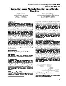
Example of genotypes and corresponding haplotypes.

Let T be the set of tag SNPs and fT (i, j) be equal to the predicted value of SNP j on genotype i using only the set T. Similarly, let AT (i, j) = 1 when fT (i, j) = gi,j and AT (i, j) = 0 otherwise. Hence, the prediction accuPi Pj racy (PA) of a set T is given by PA(T) = AT (i, j) over all i and j. 2.1

a set of n individuals with genotypes of length L (over L SNPs), we represent genotypes by an n ∗ L table and haplotypes by a 2n ∗ L table. Fig. 1 shows an example.

Multi-marker linkage disequilibrium

When using multi-marker LD, we restrict our attention to LD values between a pair of SNPs and a third marker. We denote this value by LD(S,k) (|S| = 2) which is calculated as follows (Liu et al, 2010): LD(S, SNPk) = LD({i, j}, k) = (P(XY)− P(X)P(Y))2 /P(X)P(x)P(Y)P(y)

Let Y and y be major and minor alleles of SNP k, respectively. The combination of SNPs i and j forms a group of haplotypes H. These haplotypes are subdivided into groups X and x such that: - H ∈ X if P(HY) > P(Hy) - H ∈ x otherwise Thus, the SNP set S is converted to a bi-allelic marker with two virtual alleles X and x. Then, P(XY) = Σ P(HY) for all H in X, P(X) = Σ P(H) for all H in X, etc.. 2.3

Prediction power

We propose a third measure denoted by Prediction Power PP(S, k) which estimates how well a group of SNPs S can predict SNP k. PP is based on knowledge discovery techniques which consist of mining frequent patterns and generating association rules. Again, we restrict our attention to finding interesting rules of the form {SNPx, SNPy} => SNPz. Similarly to LD calculations, we base this measure on haplotypes instead of genotypes. Therefore, every SNP triplet has 23 = 8 possible item-sets since each SNP is either 0 or 1. So, there exists 8 possible association rules between SNPs i, j and k ({0,0} => 0, {0,0} => 1, {0,1} => 0, etc.). PP(S, k) = confidence({0, 0} => 0)+ confidence({0, 0} => 1) + · · · + confidence({1, 1} => 1)

4

Interdiscip Sci Comput Life Sci (2014) 6: 1–9

where ‘confidence’ is the conditional probability P(0|{0,0}). PP(S, k) is then normalized to be in the range [0, 1]. 2.4

Linkage coverage

We define Linkage Coverage LC(SNPi, S) as the linkage coverage of SNPi over a set of SNPs S. This value is calculated by Σ LD(SNPi, SNPj) / |S| for all j ∈ S. In other terms, it is the average LD value between SNPi and every other SNP in S. In addition to its traditional usage, LC is used in the following 3 different contexts: • Two-marker TM-LC(T, S): For every SNPj in S, we find the SNPi in T such that LD(i,j) (linkage disequilibrium) is maximized. Summing up all these values and dividing by |S|, we obtain TM-LC(T, S). • Multi-marker MM-LC(T, S): For every SNPk in S, we find the pair {SNPi, SNPj} in T such that LD({i,j}, k) (linkage disequilibrium) is maximized. Summing up all these values and dividing by |S|, we obtain MM-LC(T, S). • Prediction-power PP-LC(T, S): For every SNPk in S, we find the pair {SNPi, SNPj} in T such that PP({i,j}, k) is maximized. Summing up all these values and dividing by |S|, we obtain PP-LC(T, S). The first measure, LC(SNPi, S), is used as an estimate of how well an SNPi covers the set S in terms of linkage disequilibrium. The remaining measures are required for the three different versions of our genetic algorithm and are discussed in Section 4.

3 Problem formulation Let L be a set of SNPs from which we wish to obtain a set T of tag SNPs. Let G = (V, E) be a complete undirected weighted graph such that V = L (there exists a one-to-one mapping between the vertices of the graph and the set L of SNPs). We denote by w(uv) the weight of edge uv. Since G is complete, E represents binary relationships between every pair of SNPs. The weight function can have several definitions. For example, w(uv) could be equivalent to LD(u, v) or w(uv) = F(u, v) where F is any quantity representing how good SNP v can be inferred from u or vice-versa. TSS asks for a minimum subset T satisfying the following properties: T dominates V - T (or L - T), |T| is minimized, and the summation of w(uv) for every u in T and v in V – T is maximized. The latter property can be neglected if a threshold is specified so that every edge uv whose weight is less than the threshold is deleted. This reduces TSS to the well-known NP-Complete Minimum Dominating Set problem (Sham and Cherny, 2011) which means that exact solutions are very hard to obtain especially on large instances. Note that a similar formulation still applies even if we consider multi-marker LD. The only difference is that V would be partitioned into two independent sets R and B (bipartite graph) where

R contains a vertex for every pair (or triplet) of SNPs, and B = L (the set of all SNPs). In this work, we use a slightly different formulation to the general problem. Given a parameter k, genotypes and haplotypes over L SNPs, we find a set T such that: |T| = k, which is less than or equal to L, and the coverage of T over L - T is maximized. We propose three different measures for coverage: two-marker linkage coverage TM-LC(T, L-T), multi-marker linkage coverage MM-LC(T, L-T), and prediction-power linkage coverage PP-LC(T, L-T).

4 Hybrid genetic algorithm Genetic algorithms (GAs) were developed by John Holland (Holland, 1992). They are based on the operations of population reproduction and selection for the purpose of achieving optimal results. Through artificial evolution, successive generations search for fitter adaptations in order to find optimal or good sub-optimal solutions. Each generation consists of a population of chromosomes, and each chromosome represents a possible solution. The Darwinian principle of reproduction and survival of the fittest and the genetic operations of recombination and mutation are used to create a new offspring population from the current population. The process is repeated for many generations with the aim of maximizing the fitness of the chromosomes. In this section, we present the main modules of our hybrid GA. Most of these modules are similar for the three versions of our algorithm and they include the chromosome encoding scheme, selection, crossover, mutation operations, population repair, and elitism with local improvement. The difference lays in the fitness function definition and prediction accuracy calculations. Fig. 2 depicts the sequence of steps taken by our hybrid GA. 4.1

Chromosome encoding scheme

We represent a chromosome for the Tag SNP Selection problem with a binary vector. A chromosome, denoted by Ci , is a sequence over {0, 1}L where L is the number of SNPs given in the input data. 0 represents a non-tag SNP and 1 represents a tag SNP belonging to T the set of tag SNPs. In a population P of size p we have Ci = {ci1 , ci2 ,ci3 , · · · , ciL } and cij is an element of {0, 1} where i = 1, 2, 3, · · · , p and j = 1, 2, 3, · · · , L. For example, assume chromosome Ci = 1,0,0,1,1,0 of 6 SNPs. From this encoding we can conclude that the number of tag SNPs is equal to 3, which are SNPs 0, 3 and 4 that belong to T. 4.2

Selection, crossover and mutation operations

Our selection mechanism is based on a ranking technique. Given a population P of p chromosomes and two

Interdiscip Sci Comput Life Sci (2014) 6: 1–9

5

Initial population

rate. Assume we want to crossover chromosomes Ci and Ci+1 . First, a random fraction between 0 and 1 is generated. If the fraction is greater than Xrate no crossover occurs and we move to the next pair. Otherwise, we generate two random integers, r1 and r2 between 0 and L-1 where L is the number of SNPs. Then we swap the interval [r1 ; r2 ] between the two chromosomes. For example, when Ci = 1,0,0,1,1,0, Ci+1 = 0,1,0,1,0,0, r1 = 0 and r2 = 2 the resulting chromosomes become Ci = 0,1,0,1,1,0 and Ci+1 = 1,0,0,1,0,0. In our experimental runs, we set Xrate to 0.8. Finally, the mutation procedure is executed on every SNP value (cij ) of every chromosome independently. Mutation is an essential part of any GA since it prevents premature convergence of the population. We used a mutation rate Mrate of 0.01 in this work. For every SNP of every chromosome, a random fraction between 0 and 1 is generated. If the rate is greater than Mrate no mutation occurs. Otherwise, the inclusion/exclusion value of this SNP is flipped (i.e., a 0 becomes a 1 and vice-versa). Note that crossover and mutation operations may generate illegal offspring which we deal with in the next section.

Start

Calculate fitness

Selection

Tag SNP set prediction accuracy

Crossover

Mutation End Repair

Elitisim local improvement Y

Fig. 2

Termination criteria met?

N

Flowchart representing the main steps of the GA.

4.3 user-parameter values Wdown and Wup , chromosomes are first sorted in increasing order such that the fitness value of the last chromosome is the greatest. The range between Wdown and Wup is divided into equal slots such that the number of slots is equal to the number of chromosomes. The best chromosome (having the greatest fitness value) is assigned rank Wup and the worst is assigned rank Wdown . The remaining chromosomes are assigned ranks between Wdown and Wup depending on their fitness values. In this work, we set Wdown = 0.8 and Wup = 1.2, in line with a previous successful genetic algorithm application (Mansour and Fox, 1994). The objective of this choice of values is to limit the differentiation among the pre-ranked values and, thus, provide more fair survival chances. The selection procedure copies all chromosomes having a rank greater than 1 to the next generation and then subtracts 1 from their current rank. The rank is used as a probability. When the rank is less than 1, a random fraction between 0 and 1 is generated and the chromosome is selected if the fraction is less than or equal to its rank. The process stops when p chromosomes are selected. This technique ensures that good chromosomes are selected at least once, while the other chromosomes still have a fair chance of being selected which helps keeping a diversified population. The selection operation is followed by crossovers which occur between randomly selected pairs of chromosomes. We implemented the well-known two-point crossover technique with Xrate denoting the crossover

Population repair procedure

Since we are dealing with a parameterized version of the Tag SNP Selection problem, chromosomes should have exactly k tag SNPs, where k is a user-parameter provided at startup. The initial population is generated stochastically. Genes are randomly set to 1 until a total of k genes are set to 1. After the crossover and mutation operations are performed on the population, a repair procedure considers every offspring separately and corrects every chromosome having more or less than k tags. When the number of tags in a chromosome is less than k, we randomly select additional tags until the value of k is satisfied again and the opposite is done when the number of tags is greater than k. 4.4

Fitness function

The core of our GA lies in its fitness function. The fitness of a certain chromosome, Ci , is denoted by Fitness (Ci ) and is defined for each algorithm as follows: - For GA-TMLD, Fitness(Ci ) = TM-LC(T, L - T) - For GA-MMLD, Fitness(Ci ) = MM-LC(T, L - T) - For GA-MMPP, Fitness(Ci ) = PP-LC(T, L - T) where T denotes the set of tag SNPs extracted from Ci and L - T is the remaining non-tag SNPs. In the three versions of the GA, we aim at maximizing Fitness (Ci ). 4.5

Elitism, local improvement, and termination criterion

A final technique employed in all versions of our algorithm is the concept of elitism. This technique consists of re-inserting the best-so-far chromosome into the population following every complete iteration. In addition,

6

Interdiscip Sci Comput Life Sci (2014) 6: 1–9

we introduce a local improvement module that tries to further increase the elite’s fitness value. In order not to negatively affect performance, the local improvement module restricts its attention to a specific set of SNPs. Before starting the evolutionary process, we calculate LC(SNPi, L) for each SNPi in L. LC is linkage coverage defined in Section 2.4 as Σ LD(SNPi, SNPj) / | L | for all j ∈ L. The greater the “linkage coverage” of an SNP, the more likely it is to be in T, the set of tag SNPs. After every iteration, the best chromosome is extracted and the algorithm tries to improve it by replacing one of its selected tag SNPs by another non-tag SNP that has at least as much “linkage coverage”. When this replacement increases the fitness value, the change is accepted and the number of local improvements is incremented. Otherwise, the change is rolled back. The purpose of incrementing the number of local improvements is also related to performance. A user-parameter denoted by NLI (number of local improvements) is required and whenever NLI is reached, the local improvement module terminates. Note that in some cases, no improvements are possible so the module stops after trying all possibilities. In our experiments, we heuristically set the value of NLI to 10, which allows for a fair number of improvements without causing a large increase in execution time. The whole evolution process of our genetic algorithms terminates if the best-so-far fitness value does not improve over 5 successive iterations. 4.6

Prediction accuracy

Once the termination criteria are met, the algorithm proceeds by calculating the prediction accuracy of the best solution found during the evolutionary process. Let function fT (i, j) be equal to the predicted value of SNP j on genotype i using only the set of known tag SNPs T. Similarly, we let AT (i, j) = 1 when fT (i, j) = gi,j and AT (i, j) = 0 otherwise. In other terms, Pi Pj AT (i, j) over all i and j is the sum of correctly predicted non-tag SNPs. The prediction accuracy of a certain solution, denoted by PA(Ci ), is given by: PA(Ci ) =

Xi Xj

AT (i, j)/Numberofpredictions

This definition of prediction accuracy is similar to the scoring function given in Halperin et al. (2005). The major difference between our method and the one presented in STAMPA is in the implementation of the prediction function fT (i, j). The authors of the STAMPA algorithm base their prediction algorithm on a common biological observation stating that the correlation between SNPs tends to decay as the physical distance increases (Halperin et al., 2005). Thus, their algorithm predicts a non-tag SNP value using only the value of the two closest tag SNPs to it (on both sides when possible). For example, let j1 and j2 , j1 < i < j2 be the positions of the tag SNPs closest to position i on both

sides. Their prediction procedure uses a majority vote in order to determine which value is more likely to appear in position i given that positions j1 and j2 have values a1 = {0, 1, 2} and a2 = {0, 1, 2}, respectively. Two majority votes using the phased genotypes (haplotypes) determine the two different alleles of the SNP. Note that the values a1 and a2 are taken from the genotype information directly which does not introduce another level of inaccuracy due to the phasing algorithm used. For instance, if a1 = 0 and a2 = 2, they find the most likely allele given that the alleles in positions j1 and j2 are both 0, and another allele given that the alleles in positions j1 and j2 are 0 and 1, respectively. What the authors are trying to achieve in STAMPA is to predict the value of a non-tag SNP i only using the values of tag SNPs j1 , j2 that are highly correlated with i. They use physical distance as a correlation indicator. The modification that we introduce in our prediction function fT (i, j) is that instead of using the two closest SNPs to j to predict it, we use: - The two SNPs that are in highest two-marker LD with j for the GA-TMLD algorithm; - The pair of SNPs that is in highest multi-marker LD with j for the GA-MMLD algorithm; or - The pair of SNPs that has the highest prediction power over j for the GA-MMPP algorithm. In the voting phase, the leave-one-out crossvalidation technique is used. This means that the two haplotypes of the genotype whose SNP is being predicted are not allowed to vote (the values of their alleles are not added to the total count). As we shall see in the experimental results, using our techniques provides prediction accuracies better than those of STAMPA.

5 Experimental results All variations of the GA were implemented in Java. Experiments were performed on a Linux operating system Quad Core 2 GHz PC using 500M cache. Reported results are the average of five consecutive runs unless stated otherwise. To obtain phasing of genotypes, we used the GEVALT algorithm from (Davidovich et al., 2007). Three published SNP data sets were downloaded from HapMap (http://www.hapmap.org/) for evaluating the prediction accuracies achievable by our method: • ENr112. 343 SNPs genotyped in population ASW (African ancestry in Southwest USA) on chromosome 2 from position 51512208 to 52012208. The genotypes of 83 individuals were used. • ENr113. 380 SNPs genotyped in population ASW on chromosome 4 from position 118466103 to 118966103. The genotypes of 83 individuals were used. • ENm013. 683 SNPs genotyped in population ASW on chromosome 7 from position 89621624 to 90736048. The genotypes of 83 individuals were used. The user-parameters’ values for all simulations were

Interdiscip Sci Comput Life Sci (2014) 6: 1–9

7

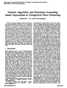
set as follows: Crossover rate = 0.8, Mutation rate = 0.01, Population size = 50, Number of local improvements (NLI) = 10, Wdown = 0.8, and Wup = 1.2. Since GA-TMLD and GA-MMLD both use linkage disequilibrium (two-marker and multi-marker LD) for evaluating the fitness function of chromosomes, we run the first set of simulations for comparing the best linkage coverage achieved by both algorithms using 2, 5, 10, 20, 40 and 100 tag SNPs on data-set ENr112. As shown in Fig. 3, multi-marker LD achieves considerably higher linkage coverage values. The exact values are given in Table 1. These results concur with previous work from the literature which established the fact that using multi-marker LD provides a better correlation indicator than two-marker LD (Wang and Jiang, 2008). We obtain similar results for the ENr113 (Fig. 5 and Table 3) and ENm013 data-sets.

1.00

0.95

0.90

0.85

0.80

0.75 2

Fig. 4

0.8

STAMPA GA-TMLD GA-MMLD GA-MMPP

5

10

20

40

100

GA-TMLD, GA-MMLD, GA-MMPP, and STAMPA prediction accuracy values with respect to the number of tag SNPs, on data-set ENr112.

0.7 0.6 0.5 0.8 0.4 0.7

0.3 0.2 0.1 0

Fig. 3

0.6

GA-TMLD GA-MMLD 2

5

10

20

40

0.5 100

GA-TMLD and GA-MMLD Linkage Coverage with respect to the number of tag SNPs, on data-set ENr112.

0.4 0.3 GA-TMLD

0.2

GA-MMLD

Table 1

Comparison of GA-TMLD and GAMMLD best fitness values using different number of tag SNPs on data set ENr112 GA-TMLD Max

GA-MMLD Max

Fitness

Fitness

2

0.1261

0.1420

5

0.1961

0.2517

10

0.2565

0.3406

20

0.3497

0.4549

40

0.4362

0.6103

100

0.5862

0.7603

# of Tag SNPs

We also compare prediction accuracies for all variations of our GA algorithm in addition to the STAMPA algorithm. From Fig. 4, we conclude that GA-MMLD outperforms all three in terms of prediction accuracy on data-set ENr112. Table 2 provides accurate readings for all simulations which places GA-MMLD in first

0.1 0 2

Fig. 5

5

10

20

40

100

GA-TMLD and GA-MMLD Linkage Coverage with respect to the number of tag SNPs, on data-set ENr113.

position, GA-MMPP second, STAMPA third, and GATMLD came in last. The results reported in Fig. 6 and Table 4 on the data-set ENr113 yields the same result, showing the best performance by GA-MMLD again. Table 5 also confirms the finding that GA-MMLD produces sets of tag SNPs which can predict the remaining non-tag SNPs with minimum error for the third data set ENm013. A major drawback of both the GA-MMLD and GAMMPP algorithms is time complexity. Calculating linkage coverage MM-LC(T, S) or MM-PP(T,S) alone runs in O(n3 ) where n is the number of tag SNPs. When |T|

8

Interdiscip Sci Comput Life Sci (2014) 6: 1–9

Table 2

Comparison of STAMPA, GA-TMLD, GA-MMLD, and GA-MMPP prediction accuracy using different number of tag SNPs on data set ENr112

# Tag SNPs

STAMPA

GA-TMLD

GA-MMLD

GA-MMPP

2

0.831007

0.8372

0.8422

0.8387

5

0.857364

0.8574

0.8598

0.8672

10

0.881309

0.8694

0.8868

0.8841

20

0.90436

0.8897

0.9123

0.8923

40

0.921826

0.9217

0.9317

0.9294

100

0.944866

0.9503

0.9603

0.9529

Table 3

0.98 0.96

Comparison of GA-TMLD and GAMMLD best fitness values using different number of tag SNPs on data set ENr113

0.94 # Tag SNPs

0.92

GA-TMLD Max

GA-MMLD Max

Fitness

Fitness

0.90

2

0.1206

0.1434

0.88

5

0.1815

0.2561

10

0.2475

0.3356

0.86

20

0.3551

0.4342

0.84

40

0.4375

0.5888

100

0.5775

0.7123

STAMPA GA-TMLD GA-MMLD GA-MMPP

0.82 0.80 0.78 0.76 1

Fig. 6

2

3

4

5

6

GA-TMLD, GA-MMLD, GA-MMPP, and STAMPA prediction accuracy values with respect to the number of tag SNPs, on data-set ENr113.

Table 4

is set to 100, it takes an average of 20 minutes for the algorithm to terminate on relatively small data-sets (less than 1000 SNPs) such as those we considered so far. For genome-wide tag SNP selection, there are around 4 million SNPs to consider and the number of tags required for reaching acceptable prediction accuracies might be in the order of thousands, which invites parallel implementation of our algorithm.

Comparison of STAMPA, GA-TMLD, GA-MMLD, and GA-MMPP prediction accuracy using different number of tag SNPs on data set ENr113

# Tag SNPs

STAMPA

GA-TMLD

GA-MMLD

GA-MMPP

2

0.8367

0.8335

0.8380

0.8378

5

0.8626

0.8556

0.8705

0.8646

10

0.8862

0.8740

0.8906

0.8806

20

0.9092

0.9010

0.9148

0.8990

40

0.9286

0.9160

0.9343

0.9302

100

0.9501

0.9422

0.9587

0.9565

Table 5

Comparison of STAMPA, GA-TMLD, GA-MMLD, and GA-MMPP prediction accuracy using different number of tag SNPs on data set ENm013

# Tag SNPs

STAMPA

GA-TMLD

GA-MMLD

GA-MMPP

2

0.7168

0.7181

0.7198

0.7191

5

0.7175

0.7180

0.7202

0.7180

10

0.7183

0.7189

0.7248

0.7176

20

0.7195

0.7189

0.7284

0.7203

40

0.7216

0.7206

0.7309

0.7229

100

0.7270

0.7237

0.7341

0.7237

Interdiscip Sci Comput Life Sci (2014) 6: 1–9

6 Conclusion In this work, we presented an approach for selecting tag SNPs based on a hybrid genetic algorithm that incorporates different linkage coverage measures. The experimental results suggest that the multi-marker linkage disequilibrium produces the best results in terms of linkage coverage and prediction accuracy in comparison with a well-known published method and other versions of the genetic algorithm. For future work, it is clear that a parallel implementation of our method is a must for addressing sequences with more realistic lengths.

References [1] Bafna, V., Halldorsson, B.V., Schwartz, R.S., Clark A.G., and Istrail, S. 2003. Haplotypes and informative SNP selection algorithms: don’t block out information. Proc. of the 7th Int. Conf. on Research in Computational Molecular Biology, 19-27. [2] Daly, M.J., Rioux, J.D., Schaffner, S.F., Hudson, T.J., and Lander, E.S. 2001. High resolution haplotype structure in the human genome. Nat Genet 29(2), 229-232. [3] Davidovich, O., Kimmel G., and Shamir, R. 2007. GEVALT: An integrated software tool for genotype analysis. BMC Bioinformatics 8, 36. [4] Devlin B., and Risch, N. 1995. A comparison of linkage disequilibrium measures for fine-scale mapping, Genomics 29(2), 311-322. [5] Gabriel, S.B., Schaffner, S.F., Nguyen, H., Moore, J.M., Roy, J., Blumenstiel, B., Higgins, J., DeFelice, M., Lochner, A., Faggart, M., Liu-Cordero, S.N., Rotimi, C., Adeyemo, A., Cooper, R., Ward, R., Lander, E.S., Daly, M.J., and Altshuler, D. 2002. The structure of haplotype blocks in the human genome. Science 296, 2225-2229.

9

[11] Ke, X., and Cardon, L.R. 2003. Efficient selective screening of haplotype tag SNPs, Bioinformatics 19, 287-288. [12] Kimmel, G., and Shamir, R. 2005. GERBIL: Genotype resolution and block identification using likelihood. Proc. Natl Acad Sci USA 102(1), 158-162. [13] Liu, G., Wang, Y., and Wong, L. 2010. FastTagger: an efficient algorithm for genome-wide tag SNP selection using multi-marker linkage disequilibrium. BMC Bioinformatics 11, 66. [14] Mansour, N., and Fox, G.C. 1994. Parallel physical optimization algorithms for allocating data to multicomputer nodes. Journal of Supercomputing 8(1), 53-80. [15] Qin, Z.S., Gopalakrishnan S., and Abecasis, G.R. 2006. An efficient comprehensive search algorithm for tag SNP selection using linkage disequilibrium criteria. Bioinformatics 22(2), 220-225. [16] Sham, P.C., and Cherny, S.S. 2011. Genetic architecture of complex diseases. In Zeggini, E., and Morris, A. (Ed.): Analysis of Complex Disease Association Studies, 1-14, Elsevier. [17] Sicotte, H., Rider, D.N., Poland, G.N., Dhiman, N. and Kocher, J.P.A. 2011. SNPPicker: High quality tag SNP selection across multiple populations. BMC Bioinformatics 12, 129. [18] Stram, D.O., Haiman, C.A., Hirschhorn, J.N., Altshuler, D.L., Kolonel, N., Henderson, B.E., and Pike, M.C. 2003. Choosing haplotype-tagging SNPs based on unphased genotype data using a preliminary sample of unrelated subjects with an example from the Multiethnic Cohort Study. Hum Hered 55(1), 27-36. [19] Thompson, D., Stram, D., Goldgar D., and Witte, J.S. 2003. Haplotype tagging single nucleotide polymorphisms and association studies. Hum Hered 56(1), 48-55.

[6] Halperin, E., Kimmel, G., and Shamir, R. 2005. Tag SNP selection in genotype data for maximizing SNP prediction accuracy. Bioinformatics 21, Supp l 1.

[20] Wang, W., and Jiang, T. 2008. A new model of multimarker correlation for genome-wide tag SNP selection. Genome Inform 21, 27-41.

[7] He, J., and Zelikovsky, A. 2006. MLR-tagging: informative SNP selection for un-phased genotypes based on multiple linear regression. Bioinformatics 22(20), 2558-2561.

[21] Xu, Z., Kaplan, N.L., Taylor, J.A. 2007. Tag SNP selection for candidate gene association studies using HapMap and gene resequencing data. Eur J Hum Genet., 15(10), 1063-1070.

[8] He, J., and Zelikovsky, A. 2007. Informative SNP selection methods based on SNP prediction, IEEE Trans Nanobioscience 6, 60-67.

[22] Zhang, K., Deng, M., Chen, T., Waterman, M.S., and Sun, F. 2002. A dynamic programming algorithm for haplotype block partitioning, Proc Natl Acad Sci 99, 7335-7339.

[9] Holland, J.H. 1992. Adaptation in Natural and Artificial Systems, MIT Press, Cambridge, MA, USA. [10] Jun J., and Mandoiu, I. 2006. Optimal tag SNP selection for haplotype reconstruction, University of Connecticut.

[23] Zhou, N., and Wang, L. 2007. Effective selection of informative SNPs and classification on the HapMap genotype data. BMC Bioinformatics 8, 484.