features for story boundary detection in broadcast news. The detection problem is .... a text, which are quite effective when story topics have salient variations in ..... ACL, 2009. [8] J. Yamron, I. carp, L. Gillick, and P. Mulbregt, âA Hidden Markov.
Multi-Modal Feature Integration for Story Boundary Detection in Broadcast News Mi-mi LU, Lei XIE, Zhong-hua FU, Dong-mei JIANG and Yan-ning ZHANG Shaanxi Provincial Key Laboratory of Speech and Image Information Processing, School of Computer Science, Northwestern Polytechnical University, Xi’an
Abstract—This paper investigates how to integrate multi-modal features for story boundary detection in broadcast news. The detection problem is formulated as a classification task, i.e., classifying each candidate into boundary/non-boundary based on a set of features. We use a diverse collection of features from text, audio and video modalities: lexical features capturing the semantic shifts of news topics and audio/video features reflecting the editorial rules of broadcast news. We perform a comprehensive evaluation on boundary detection performance for six popular classifiers, including decision tree (DT), Bayesian network (BN), naive Bayesian (NB) classifier, multi-layer peceptron (MLP), support vector machines (SVM) and maximum entropy (ME) classifier. Results show that BN and DT can generally achieve superior performances over other classifiers and BN offers the best F1-measure. Analysis of BN and DT reveals important inter-feature dependencies and complementarities that contribute significantly to the performance gain. Index Terms—story boundary detection, story segmentation, topic detection and tracking, multi-modal, feature integration
I. I NTRODUCTION A multimedia document is usually composed of multiple segments in different semantic granularities. For example, a broadcast news audio/video episode generally contains various news stories, each addressing a central topic. Story boundary detection (or story segmentation) aims to identify where one story ends and another begins in a stream of text, speech or video [1]. It serves as a necessary precursor to various tasks, such as topic detection and tracking, information extraction, indexing, retrieval and summarization, etc. A typical broadcast news retrieval system is able to locate the particular positions in a repository that match the user’s query, but lack the ability of determining where the user-interested stories begin and end. Story boundary detection exclusively targets to this purpose. As the overwhelming proliferation of multimedia documents, automatic story boundary detection is highly in demand. Story boundary detection approaches can be categorized to detection-based [2]–[7] and model-based [8]–[10]. The former directly detects story boundaries through intuitive cues/features. Based on the features, a detector or classifier is learned to make boundary decisions. The latter models a multi-topical document and segments it into story units under some optimal criterion. For detecting story boundaries in broadcast news, various boundary features have been studied in different modalities. Word similarity measures are frequently used as boundary indicators in textual documents due to the intuitive lexical cohesion phenomena, i.e., words in a story agglomerate together
via semantic relations. TextTiling [2] and lexical chaining [3] are two typical embodiments of lexical cohesion for story boundary detection. Different from textual features that reveal topic shifts by detecting semantic variations, audio/video cues are more heuristic and rely on editorial rules [5]. News transitions are signaled by a long silence or a musical break; two announcers report news stories in turn; a studio anchor leads in a news topic and a field reporter elaborates it the detail. Originated from editorial rules, major audio/video cues include anchor-face show-up, news-title show-up, significant pause, speaker change and music [4]–[6], [11]. Despite years of research, story boundary detection is far from practical applications because of its inferior performance. Due to the complexity and generality of the problem, no particular single feature is enough to handle story boundary detection for a large volume of broadcast news. Some recent efforts have shown that integrating different features is able to significantly improve the detection performance [4]–[6], [11]. Among these previous studies, decision tree (DT) and maximum entropy (ME) model are frequently used as the boundary classification scheme. Recently, support vector machines (SVM) [5] and naive bayesian (NB) classifier [7] were adopted for story boundary detection. However, despite these tremendous efforts, we notice that a comprehensive comparison on different classifiers for multi-modal feature integration is still missing and the potential state-of-the-art story boundary detection performances remain unknown. In this paper, we present an extensive evaluation and analysis of different classifiers for story boundary detection on broadcast news. Specifically, we use a diverse set of lexical, audio and video features automatically derived from broadcast news videos, which includes frequently-used typical features and newlyreleased features [12]. We conduct extensive experimentation on six popular classifiers, including generative classifiers (DT, NB and BN) and discriminative classifiers (SVM, MLP and ME). We investigate feature effectiveness and how different features complement with each other to push forward the stateof-the-art performance of story boundary detection. II. C ORPUS We experiment with the CCTV broadcast news corpus [10], which contains 71 Mandarin broadcast news videos (over 30 hours in duration) from China Central Television. Each video is associated with a large vocabulary continuous speech recognition (LVCSR) transcript. The speech recognition error
ISBN 978-1-4244-6245-2/10/$26.00 ©2010 IEEE
420
rates for word, character and base syllable are 25%, 18% and 15.5%, respectively. We divide the corpus into two portions: a set of 40 episodes for training (1209 boundaries) and a set of 31 episodes (892 boundaries) for testing. The reference story boundaries (i.e. real story boundary positions) were manually annotated. We compare the detected story boundaries with the reference boundaries in terms of F1-measure, i.e., the harmonic mean of recall and precision. In accordance with the topic detection and tracking (TDT) standard, a detected story boundary is considered correct if it lies within a 15second tolerant window on each side of a manually-annotated reference boundary. III. S TORY B OUNDARY D ETECTION S CHEME We adopt a detection-based method that involves three stages: candidate determination, feature extraction and boundary/non-boundary classification. We first determine the boundary candidates across the broadcast news stream. The principle of this stage is to reduce the boundary search complexity and to maintain a very low miss rate of story boundaries. For the video modality, we consider all the shot boundary positions as the story boundary candidates. All the silence positions are used as story boundary candidates for the audio and text modalities. For a candidate 𝜋, a set of features is then extracted. We aim to find the boundary class ℬ𝜋∗ with highest probability given feature set ℱ𝜋 for each candidate 𝜋: ℬ𝜋∗ = arg max 𝑃 (ℬ𝜋 ∣ℱ𝜋 ), ℬ𝜋 ∈ {Bnd, Non-Bnd}. (1) ℬ𝜋
To achieve this, a classifier is trained to assign ℬ𝜋 for each candidate. IV. M ULTI - MODAL F EATURE E XTRACTION A. Lexical Features 1) Lexical Similarity: Lexical cohesion describes that a story with a central topic is created by use of words with related meanings while different topics employ different sets of words [2]. As a result, a story boundary may accord with a lexical similarity minimum. Based on this intuitive assumption, we measure lexical similarity at each candidate across the broadcast news LVCSR transcript. The cosine similarity is calculated at each candidate 𝜋 across the transcript: ∑𝑁 𝑣𝑛,𝑙 𝑣𝑛,𝑟 (2) 𝑠𝜋 = cos(v𝑙 , v𝑟 ) = √∑ 𝑛=1 ∑ 𝑁 𝑁 𝑣 𝑣 𝑛=1 𝑛,𝑙 𝑛=1 𝑛,𝑟
where v𝑙 and v𝑟 are term (e.g. word) frequency vectors for the left and right text blocks of the candidate 𝜋, respectively, and 𝑣𝑛,𝜉 is the frequency of the term 𝑤𝑛 occurred in the block 𝜉 with a vocabulary size of N. Fig. 1 shows a lexical similarity curve calculated on a CCTV broadcast news transcript, from which we can observe clear similarity valleys at story boundary positions. 2) Chaining Strength: Lexical chaining is another embodiment of lexical cohesion [3]. A lexical chain links up term repetitions. A chain starts at the first appearance of a term and ends at the last appearance of the term. Lexical cohesion leads to the fact that chains tend to start at the story beginning and terminate at the end of the story. Therefore, a high
Fig. 1. Lexical similarity curve for a CCTV transcript. Vertical red lines denote reference story boundaries.
Fig. 2. Chain strength curve for a CCTV transcript. Vertical red lines denote reference topic boundaries.
concentration of starting and/or ending chains is an indicator of story boundaries [3]. We construct lexical chains for the LVCSR transcript and measure the chaining strength at each candidate 𝜋 by 𝑐𝜋 = 𝑒𝑛𝑑(𝑙) + 𝑠𝑡𝑎𝑟𝑡(𝑟)
(3)
where 𝑒𝑛𝑑(𝑙) and 𝑠𝑡𝑎𝑟𝑡(𝑟) denote the number of chains end at the left text block and the number of chains begin at the right text block of the candidate 𝜋, respectively. Since some chains may span across the text if two news report the related or similar topics, we set up a maximal chain length and beyond which no chains are allowed. Fig. 2 plots a chain strength curve of a CCTV broadcast news clip. We can clearly observe that story boundary positions tend to have higher chain strength. 3) Global Cohesiveness-based Boundary Indicator: Lexical similarity and chain strength depict local cohesiveness of a text, which are quite effective when story topics have salient variations in lexical distribution. However, sometimes topic transitions in broadcast news are smooth and the distributional variations are very subtle. Therefore, we use another boundary indicator that directly maximizes the total cohesiveness of all story fragments split out from the text [12]. This boundary indicator can effectively catch smooth topic shifts. We define the global cohesiveness of the text as the sum of cohesiveness value of all fragments split out from it, i.e. 𝒞(𝑡𝑒𝑥𝑡) =
𝐽 ∑
𝐶𝑜ℎ𝑠𝑐𝑜𝑟𝑒(𝑓𝑗 )
(4)
𝑗=1
where 𝑓𝑗 is the 𝑗th fragment. By maximizing 𝒞(𝑡𝑒𝑥𝑡), we can achieve the optimal segmentation. Due to the linearity of the segmentation problem, the maximization can be solved by an efficient dynamic programming solution. The lexical cohesiveness of a fragment 𝑓 is mainly affected by three factors: the repetition of terms − ℛ(𝑤), the specificity of terms − 𝒮(𝑤) and the length of the fragment − 𝒜(𝑙𝑒𝑛𝑔𝑡ℎ). We combine them by
421
0
200
400
600
800
1000
1200 Time (sec)
Fig. 3. The segmentation points (blue stars) versus reference story boundaries (vertical red lines) for a CCTV broadcast news transcript.
𝐶𝑜ℎ𝑠𝑐𝑜𝑟𝑒(𝑓 ) = 𝒜[𝑙𝑒𝑛𝑔𝑡ℎ(𝑓 )]
𝐼 ∑
[ℛ(𝑤𝑖 )𝒮(𝑤𝑖 )]
(5)
𝑗=1
where 𝑤𝑗 is the 𝑗th different term of fragment 𝑓 . ℛ(𝑤𝑖 ) − The basic idea is that each pair of identical words contained in fragment 𝑓 contributes equally to the cohesiveness of 𝑓 . Thus the total contribution of a certain word 𝑤𝑖 is given by 𝐹 𝑟𝑒𝑞(𝑤𝑖 )−1
ℛ(𝑤𝑖 ) =
∑
𝑘=1
𝑘=
1 𝐹 𝑟𝑒𝑞(𝑤𝑖 ) [𝐹 𝑟𝑒𝑞(𝑤𝑖 ) − 1] 2
(6)
where 𝐹 𝑟𝑒𝑞(𝑤𝑖 ) is the term frequency of 𝑤𝑖 in fragment 𝑓 . 𝒮(𝑤𝑖 ) − We introduce a specificity factor 𝐹 𝑟𝑒𝑞(𝑤𝑖 ) , (7) 𝑇 𝑜𝑡𝑎𝑙(𝑤𝑖 ) which measures the inter-fragment discriminativity for the term 𝑤𝑖 , reflecting the fact that the term appearing in more fragments are less useful in discriminating a specific fragment. 𝑇 𝑜𝑡𝑎𝑙(𝑤𝑖 ) is the number of times that term 𝑤𝑖 occurs in the whole text. 𝒜(𝑙𝑒𝑛𝑔𝑡ℎ) − A factor is introduced to reflect the reasonable fragment length. The length factor should be decreasing and decrease slowly when 𝑙𝑒𝑛𝑔𝑡ℎ(𝑓 ) is not very large as it should not offset cohesiveness gained by the increase of word repetition. That is to say, a term occurs intermittently within a short distance can be held in a same fragment. Besides, if the fragment is much beyond the typical topic length, 𝒜(𝑙𝑒𝑛𝑔𝑡ℎ) has to provide a considerable negative effect to the cohesiveness value as a penalty factor. We find that an exponential function with a base close to 1.0 suits our needs well. Formally, the length factor is defined as 𝒮(𝑤𝑖 ) =
𝒜(𝑙𝑒𝑛𝑔𝑡ℎ(𝑓 )) = 𝛼−𝑙𝑒𝑛𝑔𝑡ℎ(𝑓 )
Fig. 4. Relative frequency histograms of pause duration for boundary and non-boundary pauses for the CCTV corpus.
(8)
where 𝛼 is a constant parameter slightly larger than 1.0. The dynamic programming algorithm finally results in an optimal segmentation on the text transcript. Fig. 3 illustrates the segmentation points (blue stars) and the reference story boundaries (vertical red lines) for a CCTV broadcast news transcript. We align each segmentation point to its nearest pause (i.e. candidate) as the boundary indicator. B. Audio Features 1) Pause Duration: Pause duration is a salient speech prosodic factor relevant to discourse structures. Speakers tend to use a long silence pause at large semantic boundaries. Broadcast news producers usually insert a silence or a music clip between consecutive news stories. Previous work has shown that pause duration (i.e. silence and music duration)
Fig. 5. Detected speaker changes (blue stars) versus reference story boundaries (vertical read lines) for a brief news session in the CCTV corpus.
is quite effective for story boundary detection in broadcast news [5], [11]. Fig. 4 shows the relative frequency histograms of pause duration for story boundaries and non-story boundaries for the CCTV corpus. We can see that story boundaries have longer pause durations. Therefore, we use the pause duration at each candidate point as an audio feature. 2) Speaker Change: Broadcast news programs usually involve various speakers, such as anchors, reporters and interviewees, etc. Some news sessions are hosted by two anchors and they report news in turn. For example, in the CCTV brief news session, a male anchor and a female anchor usually alternate with each other to announce news. Fig. 5 shows the detected speaker changes for a brief news clip. We can clearly see that almost every story boundary is associated with a speaker change. Some news programs follow a clear syntax: a news story is led in by an anchor in the studio, and then followed by a detailed report from a field reporter or an interview. Therefore, in broadcast news, speaker changes may coincide with story transitions. We use a two-stage multi-feature integration approach [13] to automatically detect speaker changes from broadcast news audio. Speaker change is used as a binary feature (change/non-change for each candidate). 3) Speech Type: According to the editorial rules of broadcast news, studio-to-field transitions may coincide with news boundaries; a news story usually starts from clean speech (e.g. anchor speech in studio) and rarely start from noisy speech (e.g. field speech). Studio speech is clean in general while field speech is often contaminated with diverse background noises from news scenes such as streets, factories and buildings, etc. Therefore, speech type may indicate potential story boundaries. We use the speech type of the right side of a candidate point as a discrete audio feature (pure speech, speech with noise, speech with music).
422
Fig. 7. Appearance of detected title captions (blue boxes) versus reference story boundaries (vertical read lines) for a CCTV news episode.
V. E XPERIMENTS
Fig. 6. Anchor face counts (blue bars) versus reference story boundaries (vertical red lines) for a CCTV news episode.
A. Experiment Setup
C. Video Features 1) Shot Boundary: A shot is a continuous strip of motion pictures, consisting of a series of frames. In broadcast news video, story transitions usually happen at a shot boundary. Therefore, it is reasonable to detect whether there is a shot change at a story boundary candidate. We measure block histogram difference between two adjacent video frames to decide whether a shot boundary exists. First, a frame 𝑘 is divided into 𝑀 × 𝑁 blocks and gray-scale histogram h(𝑚, 𝑛, 𝑘) is calculated for each block (𝑚, 𝑛). The histogram difference between frames 𝑘 and 𝑘 + 1 is calculated by 𝐷(𝑘, 𝑘 + 1) =
𝑁 𝑀 ∑ ∑
∣h(𝑚, 𝑛, 𝑘) − h(𝑚, 𝑛, 𝑘 + 1)∣. (9)
𝑚=1 𝑛=1
A shot boundary is detected if the calculated distance 𝐷(𝑘, 𝑘+ 1) is larger than an empirically set threshold. 2) Anchor Face: With regards to the structural rules of broadcast news, quite a number of news stories begin with a studio anchor shot and then move to field shots. Previous research shows that anchor face presence is an important visual cue for story boundary detection [4], [5], [6]. We first use an AdaBoost detector to detect human faces in video frames, and then use a regression classifier to discriminate anchor faces from other detected non-anchor faces. Based on the characteristics of anchor appearances, e.g., face coordinates and size, the classifier labels video frames with anchor counts (0,1,2). Fig. 6 shows the anchor face counts for a CCTV news episode. We can clearly see the anchor count changes at some story boundary positions. Therefore, we use inter-frame anchor count difference at a candidate position as a visual feature for story boundary detection. 3) Title Caption: In broadcast news video, a news story is often accompanied by a caption describing the title of the news. Hence, the appearance of a title caption is a clear story boundary indicator. We detect title captions from broadcast news video based on caption region’s color and structural information. Since the title caption usually comes out later than the news and lasts for a short period, we employ a pair of numeric values to characterize this feature: distance from a candidate to its right nearest title caption appearance and the time duration of the title caption. In Fig. 7, the blue boxes indicate the appearance of title captions and their durations. We can clearly see that almost every story boundary is associated with a right-side appearance of a title caption.
We experimented with feature sets from a single modality (L,A,V) and integrated feature sets from multiple modalities (L+A, L+A+V), summarized in Table I. Note that the position of the candidate (to the beginning of the broadcast news episode), namely Pos, was inserted into all the feature sets in the experiments. The Pos feature was used as a timedependent heuristics. Table II reports the accuracies of our shot boundary detection, anchor counts, caption detection, speech type detection and speaker change detection, which are tested on an extra validation set from the same broadcast news source (CCTV). We chose the silence and music positions (labeled by the LVCSR and an audio classifier) as story boundary candidates for all the experiments except video feature experiments (V). Instead, shot boundaries were selected as story boundary candidates for video feature experiments. This ensures the videoonly experiments do not rely on an audio/lexical candidate (pause). After extraction, features such as GlbCoh, SpkChg and ShotBnd need to be aligned to an appropriate candidate since they are not likely to show up exactly at a corresponding pause. We aligned boundaries reported by GlbCoh to their nearest candidates. A shot boundary was also aligned to its nearest pause. Speaker change points were matched with their left nearest candidates due to a detection delay [13]. Note that all the lexical features were calculated on character unigram sequences for the Mandarin LVCSR transcripts due to the robustness of sub-word to speech recognition errors [10]. We tested several popular classifiers, i.e., C4.5 decision tree (DT), Bayesian network (BN), naive Bayesian classifier (NB), RBF-kernel support vector machines (SVM), multi-layer perceptron (MLP) and maximum entropy classifier (ME). The Weka toolkit (downloaded from http://www.cs.waikato.ac.nz/ml/weka/) was used to train DT, BN, NB, SVM and MLP classifiers and ME classifier was trained using the opennlp.maxent package (downloaded from http://maxent.sourceforge.net/). Since features may be redundant and some features may have low discriminativity, we performed a feature selection procedure to achieve the optimal feature subset with highest F1-measure. We adopted the backward elimination algorithm to seek the optimal subset by iteratively eliminating features whose absence do not decrease performance. All the parameter tuning, classifier training and feature selection were fulfilled on the training set. Experimental results are reported on the testing set.
423
TABLE III E XPERIMENTAL RESULTS IN TERMS OF F1- MEASURE FOR DIFFERENT FEATURE SETS AND CLASSIFIERS . L+A+V∗ : FEATURE SELECTION PERFORMED . Classifier
Lexical
Acoustic
Visual
L+A
L+A+V
L+A+V∗
Removed in feature selection
DT
0.5938
0.7133
0.7349
0.7673
0.8011
0.8103
ShotBnd AchrCnt ChStr
BN
0.6498
0.7185
0.6761
0.7644
0.8305
0.8335
SpTyp ShotBnd
NB
0.6491
0.7149
0.6188
0.7451
0.8097
0.8190
LexSim AchrCnt
MLP
0.6176
0.6926
0.6116
0.7679
0.7865
0.8029
SpTyp
SVM
0.6077
0.5540
0.4765
0.6976
0.7027
0.7105
CapDur AchrCnt LexSim SpTyp SpkChg
ME
0.5617
0.5691
0.6278
0.6685
0.7201
0.7330
CapDur ShotBnd SpTyp
TABLE I L EXICAL , AUDIO AND VIDEO FEATURE SETS USED IN THE EXPERIMENTS . Set
Feature
Abbreviation
Value
Lexical
Lexical Similarity Chain Strength Global Cohesiveness
LexSim ChStr GlbCoh
Continuous Continuous Binary
Audio
Pause Duration Speaker Change Speech Type
PseDur SpkChg SpTyp
Continuous Binary Triple
Shot Boundary Anchor Count Caption Distance Caption Duration
ShotBnd AchrCnt CapDist CapDur
Binary Triple Continuous Continuous
Video
TABLE II T HE ACCURACY RATES OF FEATURE EXTRACTION METHODS . Feature
ShotBnd
AchrCnt
Caption
SpTyp
SpkChg
Accuracy
0.935
0.967
0.948
0.96
0.813
B. Results and Discussions Experimental results are summarized in Table III. We notice that the best F1-measure for the lexical feature set (L), the audio feature set (A) and the video feature set (V) are 0.6498, 0.7185 and 0.7349, respectively. This shows that the features from three modalities can achieve comparable story boundary detection performance. When three feature sets are combined, F1-measure is increased to 0.8305. After feature selection, the performance is further increased to the highest F1-measure of 0.8335. Specifically, the integration of lexical and audio features (L+A) also achieve a pretty good F1-measure with 0.7679. We believe the complementarity between features from different modalities contributes to the considerable performance gain. When comparing different classifiers, we observe that DT and BN achieve superior performances over other classifiers in general. We notice that BN exhibits the best performance for story boundary detection, and SVM and ME show inferior performance as compared with other classifiers. Besides their outstanding performances, BN and DT offer the advantage of visual interpretability of features. We can interpret feature behaviors, their dependencies and interactions by observing the automatically learnt graph and tree. Bayesian network, a directed acyclic graph (DAG), represents a set of random variables (features) and their conditional dependencies. BNs are potentially valuable to take into account the inter-dependencies among the variables that
Fig. 8.
The Bayesian network for L+A+V∗ multi-feature set.
facilitates effective decision-making process. Fig. 8 demonstrates the BN graph achieving the best story boundary detection performance. We can easily understand the semantic dependencies among features by observing whether arcs exist between different features. We notice that features from the same modality are naturally grouped together through interfeature dependencies. Specifically, node ChStr is connected with node LexSim through a direct arc. This makes sense because a lower lexical similarity with a stronger chaining strength reinforces the probability that a topic shift takes place. A similar structural relation happens between node SpkChg and PseDur. Speaker change occurs more likely with a longer pause duration accompanied. Decision trees have been extensively used in various event detection tasks, including prosody-based story boundary detection [11]. The mechanism of a decision tree, i.e., split criterion, acts closely to human thinking mode. As compared with BN, DT offers more direct and clear interpretation of feature interactions. Figure 9 (left) shows the top levels of the DT that achieves the best performance. We notice that CapDist is the top node of the tree, reflecting its importance to the boundary decision. This is easy to interpret because almost every news story is accompanied by a news title. We also can observe the complementarity between features from different modalities. This may be summarized in terms of some major heuristic rules. For example, Path A in Fig. 9 comes out naturally: the occurrence of a speaker change near the end of the episode (Pos>1076) enhances the boundary
424
Fig. 9.
The decision tree for L+A+V∗ multi-feature set.
decision making when a candidate is close to the beginning of a title caption (CapDist