Multi-Modal Utile Distinctions - Semantic Scholar

M ULTI -M ODAL U TILE D ISTINCTIONS

Multi-Modal Utile Distinctions William Dabney

WDABNEY @ CS . UMASS . EDU

Department of Computer Science University of Massachusetts Amherst, MA 01003

Amy McGovern

AMCGOVERN @ OU . EDU

School of Computer Science, University of Oklahoma, Norman, Ok 73019 USA

Technical Report UM-CS-2010-065

Abstract We introduce Multi-Modal Utility Trees (MMU), an algorithm for autonomously learning decision treebased state abstractions in Partially Observable Markov Decision Processes with multi-modal observations. MMU builds the trees using the Kolmogorov-Smirnov statistical test. Additionally, MMU incorporates the ability to perform online tree restructuring, enabling it to build and maintain a compact state approximation. It then uses reinforcement learning over these abstractions to learn a control policy. We empirically evaluate the performance of MMU on the Tsume-Go subtask of Go, and show knowledge transfer from the single step Tsume-Go task to the multi-step Tsume-Go task. In the single step task MMU outperforms the best existing decision tree based methods and performs competitively with a Support Vector Machine method for solving Tsume-Go problems. We are unaware of existing work on multi-step Tsume-Go, but MMU reaches over 40% accuracy on subsequent gameplay steps. A random agent would achieve less than 9%, and thus there is a significant amount of knowledge transfer. The use of multi-modal observations allows us to use a variety of observation representations which are combined to form the abstractions learned by MMU. This provides flexibility in the choice of observation representation which is lacking in existing methods for the online learning of state abstractions.

1. Introduction This paper introduces Multi Modal Utility Trees (MMU), a tree-based function approximation technique for Partially Observable Markov Decision Processes (POMDPs). MMU autonomously constructs a compact task-dependent state representation using multi-modal observations with independent representations for each modality. Currently, tree-based methods for online state space approximation are restricted to working with a single representation, or modality, for observations. These include: propositional representations (McCallum, 1995; Jonsson and Barto, 2000; Brafman and Shani, 2004), deictic representations (Finney et al., 2002a), and relational representations (Blockeel and De Raedt, 1997; Laer and De Raedt, 2001; Driessens et al., 2001; Dzeroski et al., 2001; Dabney and McGovern, 2007; Ramon et al., 2007). MMU generalizes these past approaches to handle multiple modalities. This allows researchers to select the representation, or combination of representations which is most suitable for the desired task. The MMU algorithm autonomously builds a tree of ‘utile distinctions’ which distinguish between observations. The resulting tree contains many distinctions, with each distinction being made along a single modality of the observation. The leaves of the decision tree form a state space approximation over relevant features of the environment. Designing a state or observation space is critical to successfully applying reinforcement learning (RL) algorithms to new domains. An observation is a type of factored state descriptor, which may or may not be partially observable. Designing an observation for an RL agent first requires deciding on what representation to use. In current systems, this usually takes the form of a propositional, deictic, first-order, or relational graph based representation. Different domains lend themselves to different representations, and often can be 1

DABNEY & M C G OVERN

described most readily by a combination of different representations. For example, a robotic agent’s visual perceptions may be best described with a relational representation, while its built in GPS would be best described with a propositional representation. Multi-modal representations provide more control and flexibility in how observations are designed and sent to the agent. The use of multi-modal observations has advantages even when only a single form of representation is used. Consider using both high-level and low-level relational observations in a two player board game such as the game of Go. The high-level relational observation provides useful abstractions such as the Common Fate Graph (CFG) (Graepel et al., 2001). The low-level relational representation provides the details of the board by directly representing a portion of the board as stones connected through adjacency. Together, these form a multi-modal observation which provides both a high-level and low-level relational view of the Go board. This type of observation provides the agent with prior knowledge about useful highlevel abstractions, while allowing the agent to maintain access to low-level details of the domain. Multi-modal observations provide the flexibility to learn on observation representations which are best suited to the domain and task to be solved. Representation, both external in the form of observations and internal in the form of a state approximation, is a central concept of this work. The choice of representation directly affects the range of learnable concepts. Many methods rely upon a propositional representation for observations. This can be viewed as a vector of feature value pairs, which, while robust and well suited for many domains, is not a suitable representation for all domains. Specifically, there are many domains which are inherently relational, in that they are best represented by relational observations such as an attributed graph (McGovern et al., 2003), or using a first order representation (Dzeroski et al., 2001). Relational domains can be difficult to convert into propositional observations, and doing so often discards much of the useful information represented by the domain. Because of this, there has been a great deal of recent work on learning algorithms which use relational representations and are able to learn in relational domains (Driessens et al., 2001; Dzeroski et al., 2001; Finney et al., 2002a; Dabney and McGovern, 2007; Neville and Jensen, 2007). Reinforcement learning has been most successful in domains where the full state is of a reasonable size and is provided to the agent a priori. However, when the agent is presented with observations, which are either overly descriptive or only partially representative of the state of the environment, then the performance of classic reinforcement learning techniques degrades. These are the highly related problems of distractor features and perceptual aliasing. MMU addresses the problem of disambiguating the underlying state of the environment when given too little information, too much information, or a combination of both of these by building on previous work by McCallum (1995) and Dabney and McGovern (2007). Throughout this paper we will make use of the POMDP formalism (Kaebling et al., 1998), which provides a concise model of our motivating domains. Many successful techniques have been developed to solve POMDPs when a model of the environment is provided ahead of time (Thrun et al., 2000). However, this is assumption is difficult to satisfy in many real world domains. We assume that the domain is a POMDP, that the agent has no a priori model of the environment, and that the underlying states of the environment are hidden. These are some of the same motivations for recent work on alternatives to the POMDP, namely Predictive State Representations (PSRs) (Singh et al., 2003). The PSR makes no assumptions on the form of observations, but also only uses equality of observations instead of comparing aspects of observations. This has the advantage of not relying upon any particular observation representation, but may also miss generalizations that would otherwise be available. The algorithm we introduce in this paper accomplishes these goals while allowing increased generalization by comparing not just equality of observations but the structure of observations, regardless of the observations’ representation. Early decision tree based methods for reinforcement learning in POMDPs lacked the ability to reduce an overly complex model once it has been learned. This has previously been recognized as a key area for future research by other researchers (McCallum, 1995; Jonsson and Barto, 2000; Wierstra and Wiering, 2004; Driessens et al., 2006). We previously introduced an approach (Dabney and McGovern, 2007) to modify the tree online based on Iterative Tree Induction (Utgoff, 1995). This gives gives our algorithm the ability to refine an existing model, which allows the construction of more compact state space approximations.

2


Multi-Modal Utility Trees (MMU) are a generalization of the Relational Utree algorithm to multi-modal observations. We provide a proof that, given standard assumptions, the set of ‘utile distinctions’ are sufficient for learning the optimal policy in a POMDP. We describe MMU, an anytime online reinforcement learning algorithm which uses an approximation of the utile distinction test to build a decision tree based model of the underlying state space. In keeping with the Relational Utree algorithm, MMU refines the existing decision tree through tree restructuring (Dabney and McGovern, 2007). The contributions of this paper are to emphasize the benefits of multi-modaled observations within the reinforcement learning framework. We show that, compared to single representation observations, multimodaled observations provide a better framework within which to learn state abstractions, and present the MMU algorithm as an example of what is possible within this new perspective on observation representations. We empirically demonstrate that MMU, which extends and generalizes the concepts from Utree and Relational Utree, effectively learns on these multi-modaled observations. Specifically, that when MMU learns on multi-modal observations it will do better than Utree and Relational Utree provided that the additional observation modalities provide additional information useful for the task at hand, and that MMU will perform equivalently otherwise. We also show that the state abstractions learned by MMU provide a useful foundation for learning related tasks, and thus can be used for knowledge transfer. We demonstrate through related work and empirical evidence what type of domains would benefit from multi-modal observations, and what type of domains would not. We evaluate our first claim by comparing MMU to Relational Utree on a toy domain (Wumpus World) and on a challenging domain (Tsume-Go). We evaluate our second claim by using the learned state abstractions from the first set of experiments with Tsume-Go to choose actions in a related task (Multi-step Tsume-Go). Finally, we vary MMU’s parameters and evaluate its performance in the Wumpus World domain. This provides detailed information on how robust MMU is to varriations in its parameters, and what values for these parameters work well in that domain. Tsume-Go is ideal for evaluating MMU’s ability to handle multi-modal observations in a challenging POMDP domain. Specifically, we chose to use a square observation window to keep the observation size feasible but this choice makes the game board partially observable. This is similar to the roving eye of Stanley and Miikkulainen (2004) and the fixed-size pattern area of Ramon et al. (2000). We evaluate performance with different types of multi-modal observations, and show knowledge transfer by training on single step Tsume-Go and evaluating on multi-step Tsume-Go game play sequences. In Tsume-Go, MMU learns to choose the best one step move with a 55% success rate, which is competitive with a variety of state of the art machine learning methods. We then show the learned trees demonstrate significant transfer of learned knowledge when evaluated with Tsume-Go game play sequences.

2. Multi-Modal Observations A partially observable Markov decision process is given by the tuple: hS, A, T, R, Ω, Oi, which is unknown to the agent except through samples from the sets of actions, A, observations, O, and rewards, R. The tuple hS, A, T, Ri represents the underlying Markov decision process (MDP) of the environment, where S is the set of states in the environment and T is the set of transition probabilities between any two states in S given an action in A. Ω : S × A × O → [0, 1] is the set of observation probabilities, which map a given state, action, and observation to the probability of that observation when the action is taken from the given state. In a POMDP, an agent receives an observation and reward following each action performed. Following the notation of McCallum (1995) we use the term transition instance or instance to refer to the tuple at time t denoted Tt = hTt−1 , at−1 , ot , rt i. The tuple is made up of Tt−1 , the instance at the previous time step, at−1 , the previous action executed, ot , the resulting observation, and rt the resulting reward. We allow an observation to consist of an n-tuple of dimensional observations each along a different dimension of perception, and each having independent but not necessarily unique representations. We refer to such multi-dimensional, multi-representational observations as multi-modal observations. Thus, the modality of an observation is the representation of, and dimension along which, an observation comes to the agent. Before introducing the MMU algorithm, we discuss how the choice of observation representation inherently defines how transition instances of those observations can be distinguished. 3


Propositional RedOnGreen RedOnBlue BlueOnGreen BlueOnRed GreenOnBlue GreenOnRed ...

Deictic

False False False False False True

Relational: Attributed Graph

block_in_focus block_on(block_in_focus) color(block_in_focus) = Red ...

Colin

ear

Relational: First Order Logic

Color = Green

On

Color = Red

Block(A) Block(B) Block(C) Block(D) On(A,D) Color(A,Green) Color(D, Red) Colinear(A,B,C)

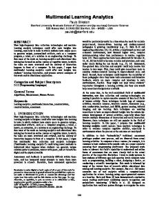
Figure 1: Example of observation representations for a blocks world 2.1 Observations Define Distinctions The MMU algorithm is a decision tree based method and relies upon distinctions to split instances at each node of the tree. In the remaining part of this section we will show how observations, regardless of representational choices, define the set of distinctions which can be used in the decision tree. Consider two distinct observations, o1 and o2 . Regardless of representation, we define o1 6= o2 if and only if there exists some aspect of o1 which is distinct from o2 . Generally, in a POMDP, we want to differentiate observations by including an arbitrarily large history window of past observations. In this case we say that o1 6= o2 if and only if there exists some aspect of o1 ’s history window of observations which is distinct from o2 ’s history window of observations. Such an aspect of an observation, which differentiates between two or more observations, is referred to as a distinction. The representation of the observation provides the aspects along which those two observations may differ. Because of this, the set of observations inherently defines a set of distinctions. Furthermore, this set of distinctions is paired to the set of observations, and specifically to the observations’ representation. Therefore, the set of distinctions defined by the observations along one dimension have no applicability to the observations of another dimension. Decision tree methods applied to first-order and attributed graph based relational representations often make use of variables defined by the distinctions in the tree to provide additional context for future distinctions (Ramon et al., 2000; Dabney and McGovern, 2007). In keeping with this past work we allow such variables, and refer to them as variable memory. Variable memories are dependent upon the tree structure and must be updated if the tree changes. In general, the variable memory created by a distinction contains a variable with the result of that distinction, which can then be referenced by future distinctions. How each type of distinction makes use of this feature will be discussed in detail below. With this in mind, as well as the concept of variable memories, we can now look at examples of the type of observation/distinction pairs possible for propositional, deictic, and relational representations. Figure 1 shows an example of each of the types of distinctions discussed below. 2.2 Propositional Observations The most common representation used for observations and state representations in reinforcement learning is propositional. In the most extreme case we can view this as a list of boolean statements about the world which indicate the state. In general, we define propositional observations, or a propositional representation as follows. A propositional observation consists of a vector of feature values, where the values may be either

continuous or discrete. We can denote this as: o = v0 , v1 , . . . , v|F| , where vi denotes the value of the ith feature and there are |F| + 1 features. These feature vectors have the advantage of being easy to understand, when |F| is small, and being well understood in the context of reinforcement learning. The set of propositional observations defines spanning sets of distinctions which are sufficient to distinguish between all distinct observations. One such spanning set of distinctions are of the form , where feature is a feature in the feature vector, threshold is a value for that feature, operator is a method for comparing values of the feature (such as ’’, ’≤’, and ’≥’), and

4


history index is the number of observations into the past to look for the observation that the distinction is applied to. The variable memory returned by a propositional distinction is simply the value of the feature in the observation. For instance, if a propositional distinction < F0, 0.75, was applied to the observation [0.55, 1.24, 0.01], where F0 indicates the first feature of the observation, then the observation would fall down the yes branch and have variable memory with the value 0.55. 2.3 Deictic Observations Deictic observations are an intermediate step between propositional observations and relational observations. Deictic observations represent the objects in a relational domain, with respect to the agent; for instance, the block that I am holding (Finney et al., 2002a). Deictic representations use egocentric pointers to reference objects in the environment as they relate to the agent. Properties of these objects can then be referenced using the pointers. This allows for some of the generalization of a relational representation, but with the added difficulty of deciding what objects the pointers should be assigned to. The advantage of deictic representations is that they can be used with existing reinforcement learning algorithms (Finney et al., 2002a; Ravindran et al., 2007). A difficulty with deictic representations occurs when the agent has control over the focus of the pointers and is simultaneously building an internal state representation (Finney et al., 2002b). For example, the object I am holding is a name for the pointer of the object being held. We can then reference properties and relationships of this object with color of(the object I am holding) or object next to (the object I am holding). These refer to the color of the object being held and the object next to the object being held respectively. Actions can also be integrated into these deictic representations, such as move toward(the object I am looking at). Variable memories for deictic distinctions are treated in the same way as with a propositional distinction. This is because a deictic representation is a special case of propositional representations. Thus, the variable memory is the value of the feature being tested, such as the value of “blue” for color of(the object I am holding). 2.4 Relational Observations: Attributed Graph We can represent a relational observation with an attributed graph, o = hV, E, A(V ), A(E)i (McGovern et al., 2003). The set V contains the vertices of the graph, which correspond to objects in the observation. Relationships between a set of objects are represented as edges, E, connecting two or more vertices of the graph. Thus, the attributed graph is a hyper-graph because the edges can connect any number of different vertices. Both objects and relationships can have continuous or discrete valued attributes, A(V ) and A(E) respectively. The Relational Utree algorithm uses a set of relational distinctions over observations represented with attributed graphs to build a decision tree based state approximation (Dabney and McGovern, 2007). These distinctions are low level, in that they only test the properties and structure of the attributed graph, without any additional processing. Relational Utree’s distinctions include existence of an object type, whether a certain type of relationship exists between a set of two objects, and attributes of an object or relationship. Because this set of distinctions are so low level, they rely upon the variable memories in order to combine multiple simple distinctions into more complex queries. We now show that these complex queries formed by Relational Utree’s distinctions are a spanning set of distinctions on attributed graphs. Distinctions made by Relational Utree are in one of the following forms: 1. Existence of objects of a certain type, with variable memory containing references to all of the objects of that type. Example: ∃ Object(ob j) such that type(ob j) = stone 2. Existence of a relationship between objects referenced by a set of variable memories. The variable memory returned by this distinction contains the relationships that match this query, as well as pointers to the related objects. Example: ∃ Relationship(rel, ob j1 , . . . , ob jn ) such that type(rel) = adjacency 3. Value of an attribute of a given object or relationship referenced through a variable memory. The variable memory returned by this distinction contains the object or relationship references which match 5


the attribute value. Example: For a object or relationship variable memory V , ∃v ∈ V such that v.color = ”red” 4. Size of the variable memory of a previous distinction. The variable memory returned by this distinction is the same as the one it references, except when the query on its size is false. Example: For a given variable memory V , |V | > 3. This will be true if the number of elements in V is greater than three, and false otherwise. Theorem 1. The set of distinctions made by Relational Utree are sufficient for distinguishing between any pair of relational observations represented using an attributed graph. Proof. Let o1 , o2 be a pair of relational observations represented using attributed graphs. For o1 and o2 to be distinct we mean that o1 6= o2 , which implies that there is one or more elements of the attributed graphs which are different between the two observations. From the definition of an attributed graph given above we construct the following exhaustive list of base cases for which o1 6= o2 , followed by the distinction which distinguishes between that case: 1. Different number of objects of some type. Let |Ob j(o1 , T )| and |Ob j(o2 , T )| be the number of objects of type T for observations o1 and o2 respectively. Then the application of the object existence distinction for type T , followed by a distinction on the size of the resulting variable memory which tests for size equal to |Ob j(o1 , T )| results in o1 and o2 falling into different leaves of the tree when |Ob j(o1 , T )| 6= |Ob j(o2 , T )|. 2. Different attribute values of objects. Let a ∈ V (o1 ) and b ∈ V (o2 ) be objects which are of the same type T , but have different attribute values on the attribute f in the two observations. An object existence distinction on type T , followed by an attribute value distinction on the attribute f equal to the value of a results in distinguishing between o1 and o2 . 3. Different relationship types between a set of objects. Using the above two cases the objects can be identified, providing variable memory pointers to each object in the relationship. Thus, for objects ob j1 , ob j2 , . . ., ob jn existing in both observations, a relationship distinction is created for type T , the type of the relationship between the objects in o1 . This distinguishes between o1 and o2 whenever the type of relationship amongst the objects is different between o1 and o2 , and when the objects in the relationship are different. 4. Different attribute values, for attribute f , of a relationship common among the two observations o1 and o2 . Follow the above case to give the variable memory referencing the relationship in question. Add an attribute value distinction, using the previously created variable memory, on the attribute f for the value of that attribute for the relationship in o1 . This distinguishes between o1 and o2 when the value of attribute f on this relationship is different. The key fact to recognize is that if observations do not differ in one of the above ways then the way in which they are intended to differ is not represented in the attributed graph. In particular, if differentiating between two observations requires the use of a special identifier or label on objects which is not included as an attribute, then observations differing in this way are identical to the agent which can only perceive the attributed graphs. Thus, the Relational Utree’s set of distinctions is sufficient for distinguishing between any pair of distinct observations represented using an attributed graph. 2.5 Relational Observations: First Order Logic Another representation for relational observations is First Order Logic (FOL). In a first order representation, the observation is given by a set of ground facts and supported by a set of background knowledge (Laer and De Raedt, 2001). An example of how a set of ground facts can represent an observation is shown in Figure 1. This type of representation has been widely used for representing relational knowledge, with extensive work 6


oi

oi+1

oi+2

oi+3

oi+4

Si

Si+1

Si+2

Si+3

Si+4

ri

ri+1

ri+2

ri+3

ri+4

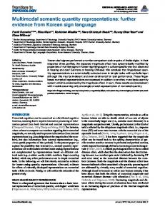
Figure 2: HMM defined by a POMDP on learning relational decision trees with first order observations (Blockeel and De Raedt, 1997; Laer and De Raedt, 2001; Driessens et al., 2001). Among these, the RRL-TG algorithm has been shown to be effective at learning in relational domains using first order representations (Dzeroski et al., 2001). When dealing with first order representations we will use the terminology and set of distinctions used by Dzeroski et al. (2001). First, we show that this set of distinctions on the first order observations is sufficient for distinguishing all first order observations. A distinction for FOL representations will test if the predicate exists, and will use variable memories for variables in the predicates. The size distinction on variable memories is not required in this case because observations can be differentiated based solely upon the predicates each one contains. Theorem 2. The set of distinctions composed of first order predicates with combinations of bound and unbound variables is a spanning set of distinctions for relational observations with a first order representation. Proof. For any two first order observations o1 and o2 , such that o1 6= o2 , there exists one or more ground facts contained in one observation and not in the other. Let this ground fact be denoted as p(X), where X is the variable or variables used in the predicate. The tree containing a distinction on p(X), along with other distinctions for X as necessary will distinguish between o1 and o2 . 2.6 Multi-Modal Distinctions Each of the representations described above can be used for multi-modal observations. Multi-modal distinctions must be able to distinguish between all unique multi-modal observations. A multi-modal observation at time t is denoted ot = hot1 , ot2 , . . . , otn i, where each dimensional observation oti has a independent representation. We then say that a multi-modal distinction is given by the pair made up of a dimensional distinction, such as one of those given above, and an index indicating which dimensional observation the distinction should be applied to. We denote a multi-modal distinction as d = hdi , ii, where di is the dimensional distinction which is applied along dimension i. The set of all such multi-modal distinctions is given by the union of the sets of dimensional distinctions, Di for each dimension i, and is denoted DM = {∪d∈Di hd, ii |1 ≤ i ≤ n}. Because each set of dimensional distinctions is sufficient to distinguish among the observations along its dimension, we can see that the set of multi-modal distinctions will also satisfy our requirement of distinguishing between all multi-modal observations. Throughout the rest of this paper, when we refer to distinctions we mean a multi-modal distinction. Additionally, each distinction will include a history index pointer which indicates a past transition instance at some arbitrarily large distance into the past.

3. Distinction Selection A POMDP defines the Hidden Markov Model (HMM) shown in Figure 2 (Kaebling et al., 1998). This HMM has state transition probabilities, P : S × A × S → R, and probability functions for emission of observations and rewards, O : S → R and R : S × A × R → R respectively. The task for our agent is to observe transition 7


instances, whose observations and rewards are generated from this HMM, and to infer an approximation to the set of states S. In doing so the agent should also be able to approximate the emission probabilities for rewards and use reinforcement learning to learn to perform a control task. Since the primary goal for our agent is to learn an optimal control policy, we want the agent to learn a state approximation which is necessary and sufficient for learning the optimal policy for a task in a given environment. As we saw above, there are distinctions which differentiate between observations. The set of all such distinctions partitions the set of observations into some maximal state approximation Smax , such that Smax ≥ S, where S is the set of states in the POMDP. As a base case we require that Smax be sufficient for learning the optimal policy of the POMDP. This reduces to our base assumption; we assume that for some arbitrarily large, finite history window of transition instances the domain becomes Markovian. The central problem addressed in this paper is the problem of selecting a set of distinctions, such that the resulting set of aliased states is minimal but still sufficient for learning the optimal policy. Ideally, this would mean the state approximation is necessary and sufficient for learning the optimal policy, but as we will soon see our method maintains sufficiency but does not guarantee necessity. We also require that the problem be solved in an online and incremental manner, allowing it to be an anytime algorithm. Finally, the state approximation should be used with a reinforcement learning algorithm to learn the optimal policy of the POMDP. 3.1 Utile Distinctions We present a solution to the above task based upon McCallum’s (1995) utile distinction test. The utile distinction test provides a method for selecting distinctions. Definition 1. “The utile distinction test distinguishes states that have different policy actions or different utilities, and merges states that have the same policy action and same utility.” McCallum (1995) We show in Theorem 4, included in the appendix, that the set of utile distinctions, those distinctions selected by the utile distinction test, are sufficient but not necessary for learning the optimal policy. We make the assumption that for some arbitrarily large history window of the observations the domain becomes Markovian. We consider this a valid assumption because the window size can be arbitrarily large, and does not need to be specified in advance. However, significant performance gains can be achieved by providing a reasonable estimate at the largest history window needed. Now, we show that this set of distinctions can be represented as a decision tree whose leaves define a state approximation which maintain sufficiency. Theorem 3. The set of utile distinctions, D, can be represented as a decision tree which defines a set of states sufficient for learning the optimal policy. Proof. For a given set of utile distinctions, D, which define a set of states D(S) sufficient for learning the optimal policy, define a discrete feature vector F. Each feature, fi ∈ F, has values defined by the branching factor of a distinction in D. Thus, fi can take values between 1 and the number of leaves in the distinction subtree di ∈ D. Then there exists a decision tree which fully divides the set of possible data points in F. Such a tree will therefore form a set leaf nodes which subsumes the set of states D(S), and is therefore sufficient for learning the optimal policy. 3.2 Areas of Approximation Because the agent must learn online, with limited experience with which to judge distinctions, we define an algorithm which is based upon the above theoretical foundations but makes approximations where necessary to learn online. With infinite experience each distinction could be judged purely by the utile distinction test. However, because the amount of experience available is limited by memory, our algorithm uses a heuristic function which approximates the utile distinction test. The heuristic is the one used by the Relational Utree algorithm, and is very similar to that used by the original Utree (McCallum, 1995; Dabney and McGovern, 2007). The heuristic is the negative logarithm of the p-values of the Kolmogorov-Smirnov statistical test

8


p(h | χ) − Using Cosines and varying values of χ 0.5

0.45

0.45

0.4

0.4

0.35

0.35

0.3

0.3

p(h | χ)

p(h | χ)

p(h | χ) = p(h) − Simple method for random history index 0.5

0.25

0.25

0.2

0.2

0.15

0.15

0.1

0.1

0.05

0.05

0

0

5

10

15

20

25

30

35

40

45

50

χ = 10 χ = 20 χ = 30 χ = 40

0

0

5

10

15

20

h

(a) p(h|χ) = p(h) =

25

30

35

40

45

h

1 2h+1

(b) p(h|χ) =

cos π∗h 2∗χ π∗i ∑hi=0 cos 2∗χ

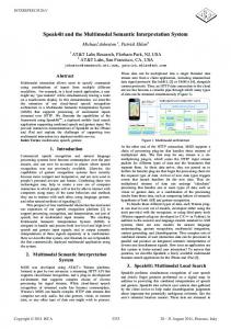
Figure 3: Comparison of the probabilities of different history indices for random sampling methods. between the expected future discounted rewards of instances in potential states. The Utree algorithm used the p-values without first taking the logarithm. We make this change to bias the values so that small p-values have greater effect on averages. Furthermore, depending upon the distinction representation, the number of possible distinctions can be large enough to necessitate the use of stochastic sampling during distinction selection. Finally, to allow arbitrary window sizes we must ensure that it is possible for any history index value to be selected. Thus, we sample values for the history index, choosing a given value h with probability p(h|χ) where χ is a bias term indicating the largest possible history index. The results given in this paper were achieved using the equation in Figure 3 (a), which is independent of the bias term. However, we note that the use of other distributions for h can improve the performance by increasing the likelihood of considering distinctions with relevant history indices. Such a potential replacement distribution is given in Figure 3 (b). The probabilities of choosing some value h are shown in the figures above each equation.

4. MMU Algorithm Based upon the above approximations to the utile distinction test and methods for generating random history indices we will now outline the MMU algorithm itself. First, we should note that Utree, Relational Utree, and MMU are essentially learning regression trees which predict distributions of future discounted rewards. The leaves of the resulting regression tree are then treated as states for a reinforcement learning agent. The intuitive reason behind doing this is that in order to maximize expected reward the reinforcement learning agent only needs to distinguish between states which have different distributions of expected future discounted reward (utility) or different optimal policies. This intuitive explanation is equivalent to the definition of the utile distinction test, which is sufficient for learning the optimal policy in a POMDP. The Utree algorithm is a decision tree based method for learning a state approximation which uses propositional observations. It builds a decision tree using the utile distinction test as a heuristic for choosing distinctions (McCallum, 1995). The MMU algorithm is similar to Utree, but requires additional steps for the tree restructuring and stochastic distinction generation. At an algorithmic level MMU differs from Relational Utree in the way that it generates random history indices, handles observations and how distinctions are applied to these observations. For the results presented here we have not strictly used Relational Utree as a comparison. Instead

9

50


we have used MMU using only the low-level relational observation representation used by Relational Utree. This is done because the comparison we are interested in is the use of multi-modal versus purely relational representations. The Multi-Modal Utility Tree Algorithm builds an approximate state space for an RL agent within the classical RL update cycle in which the environment provides an observation and reward signal to the agent, and the agent responds with an action to be taken. The basic structure of the MMU algorithm contains a very simple cycle: Generate experience and then update the tree based on these experiences. This tree forms the state abstraction for the agent where it is able to take an observation as input and output an action. The tree update reconsiders the distinctions at every node, which can result in tree restructuring. This includes considering distinctions for leaf nodes, which can also result in tree expansion. We describe this below and a detailed description is given in pseudocode in Appendix A. Multi-Modal Utility Tree uses several parameters to control its behavior. A list of these parameters and their meanings is given in Table 1.

Symbol α, k c γ ε d p ϕ maxH e

Table 1: The parameters used by MMU with a brief description of each. Description Stochastic sampling’s confidence, α, of finding a distinction in the top (k × 100)% of possible distinctions temporal sampling rate, is the number of experience steps kept for every one step ignored discount rate used during the reinforcement learning portion of the algorithm probability of choosing an exploratory action and is used by the ε-greedy action selection maximum depth of distinction trees to generate during distinction selection probability of incorrectly rejecting the null hypothesis in the Kolmogorov-Smirnov statistical test uncertainty multiplier, multiplicative decrement to uncertainty of distinction nodes found to be most utile maximum amount of experience to hold in memory at any time number of steps of experience to generate between tree updates

Multi-Modal Utility Tree Algorithm: Overview MMU is a decision tree algorithm which is trained iteratively and receives experience one step at a time. Each step of experience contains an observation, ot , and a reward, rt . Combined with the previous action performed, at−1 , this experience is used to create a transition instance, Tt = hTt−1 , at−1 , ot , rt i, to represent this step of experience. The first transition instance in an episode will not have values for Tt−1 and at−1 because no previous actions or experience exists in that episode. The transition instance is dropped down the tree using standard decision tree methods. It is then stored at the correct leaf of the tree. The state-action values are then updated using the process described below. After processing e instances, MMU performs a tree update, which updates the tree to reflect the data that has been received so far. The tree update process is described in detail below. The tree update portion of the algorithm can be viewed as learning a regression tree to estimate the expected future discounted rewards of the transition instances stored in the leaves. However, instead of rebuilding a new tree at each update, the nodes which are considered stale are re-evaluated and updated based on the experience gathered up to this point. This involves changing internal nodes of the tree, and to do this without losing the tree’s structure we have adopted the tree restructuring algorithm of Utgoff (1995). Thus, MMU goes through cycles of collecting experience using the current tree to generate actions, and then updating the entire tree based on these new experiences. Because of tree restructuring, the tree used by MMU may grow larger or smaller from update to update. Value Iteration: Update State Values ˆ a) and Pr(s ˆ 0 |s, a). These To update the state-action values the value-iteration algorithm is used with R(s, are estimated values for the reward function R(s, a) and the transition probabilities Pr(s0 |s, a), which are unknown to the agent. The update equations are given by Equations 1 - 4 (McCallum, 1995; Sutton and Barto, 1998). For these equations, s and s0 represent leaves of the decision tree, and a ∈ A is an action in the set of possible actions. Other reinforcement learning algorithms may be used instead of value-iteration, but we used value-iteration in our experiments because the tree updates require maintaining Rˆ and Pˆ and thus using value-iteration resulted in no additional memory requirements. 10


ˆ 0 |s, a)U(s0 ) ˆ a) + γ ∑ Pr(s Q(s, a) ← R(s,

(1)

U(s) = max Q(s, a)

(2)

s0

a∈A

ˆ a) = R(s,

∑Ti ∈T (s,a) ri+1 |T (s, a)|

0 ˆ 0 |s, a) = |∀Ti ∈ T (s, a) s.t. L(Ti+1 ) = s | Pr(s |T (s, a)|

(3) (4)

Multi-Modal Utility Tree Algorithm: Tree Update Updating the tree involves updating each stale node in the tree individually, which is done with Algorithm 3. A node is stale with probability equal to the node’s uncertainty if that node has been marked as potentially stale. 1. Stochasticly generate n, where n ≥ d.

ln (1−α) ln (1−k)

(Srinivasan, 1999), distinction trees up to a maximum depth

2. For each generated distinction tree φ, compute the distribution of expected future discounted rewards at each leaf node of φ and compare the distributions following the method given in McCallum (1995). This gives a set of p-values, pφ , for the Kolmogorov-Smirnov statistical tests performed. 3. Choose φbest as the distinction tree with the smallest mean log p-values on the KS-test (highest quality). 4. If the quality of φbest is not above the threshold, −1 ∗ log pks , then prune the tree at the current node, creating a leaf node in its place. Otherwise, bring φbest to replace the current node in the tree through a series of tree restructuring transpositions which will retain as much of the tree’s structure as possible. This is done by Algorithm 6, and the details of these restructuring operations are shown in Figure 16. For more information on how this is done refer to Utgoff (1995). 5. Mark φbest as not stale. If φbest was the same as the previous distinction tree at this node, then reduce the uncertainty of this distinction tree, making it less likely to be considered stale in the future. 6. Repeatedly update the state-action values until they converge. Once all nodes have been updated, then while the number of instances is greater than maxH , remove the oldest episode of experience. MMU As A Generalization of Previous Algorithms As described above, Utree is an instantiation of the MMU algorithm in which DM contains only propositional distinctions and action distinctions, and where ϕ = 0. Additionally, Relational Utree is an instantiation of MMU in which DM contains only relational distinctions and action distinctions, and where ϕ = 1.0.

5. Empirical Results As mentioned previously, the problem solved by the Multi-Modal Utility Tree algorithm is to infer a state space approximation and learn a control task on that state approximation in a POMDP with no model provided to the agent. We begin by examining performance as key parameters of MMU are varied. For this parameter search we use the Wumpus World domain. This study of how the parameters affect performance allows us to analyze the effects of different parameter values as well as the robustness of the performance to parameter value selection. We then apply this algorithm to problem domains that lend themselves to a multi-modal observation. The game of Go is a two player board game, played on a 19x19 grid. Each player places stones

11


of a single color, black for one player and white for the other, attempting to capture the opponents stones as well as capture territory on the game board. Go is a challenging problem for machine learning because of the complexity of strategies, difficult representational choices, and large branching factor (Muller, 2002; Bouzy and Cazenave, 2001). Within the Tsume-Go domain, we begin by examining MMU’s performance on the single step Tsume-Go subtask, which allows us to compare to machine learning algorithms which are the most similar to MMU (Ramon et al., 2000; Dabney and McGovern, 2007). We use the Tsume-Go domain to examine representational choices for observations, using first a simple single representation that allows the most direct comparison to related work and then using a multi-modal representation that allows the agent to take advantage of the lowlevel relational structure (stone positions), high-level relational structure (full board shapes), and high-level propositional features. We then evaluate how well these learned abstractions and value functions extend to a multiple step version of Tsume-Go in which the agent must choose successive moves, each one responding to another move by the opponent. 5.1 Wumpus World Wumpus World is a simple domain introduced by Michael Genesereth and further elaborated on by (Russell and Norvig, 1995). It is set in a grid world in which there lives a ferocious wumpus, which when encountered kills the agent. However, the agent is not defenseless against the wumpus. It has a single arrow, which when shot in the direction of the wumpus, will kill the wumpus and remove it from the world. Additionally, the world contains pits and gold. If the agent moves into a square with a pit, the agent falls to its death. If the agent moves into the square with gold on it, the agent succeeds in the task. Additionally, both the wumpus and the pits give off observable features that warn the agent that they are nearby. The wumpus has a stench that can be sensed one square away in all directions, while the pits give of breezes that can also be sensed up to one square away in all directions. Thus, the agent must learn to navigate the world, avoiding pits and avoiding or killing the wumpus, in order to find the gold. We created a multi-modal version of this domain, by making the ability to sense the breeze and stench features of a modality separate from the rest of the observation. The multi-modal observation has two dimensions. The first uses a relational representation in which the objects are empty space, the wumpus, a pit, and the gold. The relationships is the adjacency between these objects. The second dimension is a high level propositional representation, which contains the features listed in Table 2. Table 2: The propositional features used in the Wumpus domain. Feature x position of agent in grid y position of agent in grid is there a stench above the agent? is there a stench below the agent? is there a stench left of the agent? is there a stench right of the agent? is there a breeze above the agent? is there a breeze below the agent? is there a breeze left of the agent? is there a breeze right of the agent? We then used this simple domain to do a parameter search to study how variation in the parameter values affect performance. We varied the parameters used by MMU within reasonable ranges for the parameters. For instance, extremely low or extremely high values of some parameters would make learning either impossible (e = 10−50 ) or require too much time (e = 1 or d = 100). However, whenever possible we chose broad ranges in values to demonstrate the effects of the parameter on learning.

12


5.2 Wumpus World/Parameter Search Results In this section, we perform an exploration of the performance of MMU on the Wumpus World domain while varying each parameter within a range of typical values. The first variable we examine is the sample rate, c, parameter which controls how often observations are sampled. A value of −1 means sampling is disabled and all observations are used. For all other (positive) values the parameter value is how frequently observations are ignored. Thus, a value of 10 indicates that for every 10 observations received, one will be ignored by the algorithm. SImilarly, a value of 1 means that only every other observation is used. Figure 4 shows how the sample rate parameter affects performance. Interestingly, it appears that a very small amount of sampling actually leads to improved performance in this domain, while moderate amounts of sampling and none at all both outperform a parameter value of 1. This makes sense based on how we would expect this parameter to affect things. However, it is important to keep in mind that the effects of sampling are completely dependent on what the domain, and that in different domains different sample rates are more or less appropriate.

0.020 0.015

sample_rate -1.000000 100.000000 10.000000 1.000000

0.010

Y

0.005 0.000

-0.005 -0.010 -0.015 -0.0200

5000

10000 X

15000

20000

Figure 4: sample rate parameter, c As the MMU algorithm runs the tree it has learned naturally becomes more stable, and less prone to drastic changes near the root of the tree, as the algorithm finds the best possible distinctions near the root. The stability parameter allows the algorithm to back off how frequently these ’stable’ distinctions are checked for being the best distinction at that particular node. Each distinction, upon creation, is given a baseline probability (1.0) of being checked upon next tree update. Each time that same distinction is found to still be the best distinction at a particular node the probability of it being checked again is reduced by multiplying the probability by the stability parameter, ϕ. Thus, stability parameter values that are very near 1.0 lead to the tree only very slowly tending to stop checking distinctions that are very unlikely to ever change, while values near 0.0 very quickly crystalize and are no longer checked very often. A stability value of 1.0 means every node is reconsidered every tree update, while a value of 0.0 means tree restructuring is effectively disabled and nodes are never reconsidered (this is more similar to the behavior of the original Utree). Figure 5 shows how several values of this parameter affect performance. If we, for the moment, ignore the values of 1.0 13


and 0.0 there is a general trend that values nearer 1.0 perform better than values closer to 0.0. Now, for the boundary cases this pattern is reversed. We think that this is because a value of 0.0 allows for much faster tree growth, and thus many more states, which in this domain has lead to improved performance. Conversely, a value of 1.0 leads to constant uncertainty about nodes and less tree growth. Not shown here however, is the fact that run time is increased by larger values of the stability parameter. Thus, this should be considered carefully when choosing what value to use for this parameter in a given experiment.

stability 0.025 1.000000

0.020

0.990000 0.900000 0.800000

0.015

0.500000 0.000000

0.010

Y

0.005

0.000

-0.005

-0.010

-0.015

-0.020 0

5000

10000

15000

20000

X

Figure 5: stability parameter, ϕ When the MMU algorithm considers a leaf node for expansion by splitting on a new distinction at that leaf it will only consider leaf nodes which contain at least a certain number of instances. This minimum number of instances that a leaf node much have before it may be split is controlled by the minimum instances parameter. Figure 6 shows how performance changes as this is varried. It appears that for all the relatively small values (between 1 and 100) performance is about equivalent, but for the fairly large value of 1000 learning takes much longer and is slower overall than for the other values. This is reasonable because there is a direct limitation on how fast the tree can grow and how large of a tree can be grown when this parameter becomes large. The only downside to having very small (values around 1) values for this parameter is that the resulting trees may become larger than is strictly necessary to learn the concepts.

14


0.025 0.020

min_node 1.000000 10.000000 100.000000 1000.000000

0.015 0.010 Y

0.005 0.000 -0.005 -0.010 -0.015 -0.0200

5000

10000 X

15000

20000

Figure 6: minimum instances in a node parameter When deciding which distinction to use to split instances at a node the Kolmogorov-Smirnov statistical test is used. The critical value, p, is a parameter which controls at what level of statistical significance a distinction will be allowed to be used in the tree. Specifically, it is a threshold which a distinction’s p-value must be below (probability of incorrectly rejecting the null hypothesis) in order to include the distinction into the tree. Figure 7 shows a variety of values for this parameter and how performance is affected. This figure shows a very clear trend that larger values of this parameter have better performance. This may seem confusing, why would accepting distinctions into the tree that are probably not very good actually improve performance? The answer comes from one of the benefits of MMU, which is that distinctions are continually being reconsidered. So long as the agent continues to do tree updates the MMU algorithm will continue to improve on the existing tree. What unusually high values of this parameter allow the algorithm to do is essentially bootstrap its representation learning more effectively resulting in faster learning, at the cost of having a tree that is significantly larger than is required.

15


pks 0.025 0.005000

0.020

0.050000 0.100000 0.200000

0.015

0.300000 0.500000

0.010

Y

0.005

0.000

-0.005

-0.010

-0.015

-0.020 0

5000

10000

15000

20000

X

Figure 7: critical value for KS-Test, p When generating distinctions to split instances at a node the MMU algorithm begins by generating single distinctions, subtrees of depth 1, but if no statistically significant split is found at this depth (see the critical value parameter above) then the depth of subtrees generated increases by one and the process begins again. The maximum depth parameter determines what the maximum depth for these subtrees should be. For instance, a subtree of depth 3 would contain up to seven distinctions, and as few as three. Figure 8 shows what we would expect, that larger values of the maximum depth improve performance. The drawback to increasing the maximum depth parameter very much is that it significantly increases the run time because it has a multiplicative effect on both the number of distinctions generated overall as well as the number of subtrees considered for inclusion in the tree.

16


depth 0.04 1.000000 2.000000 3.000000

0.03

Y

0.02

0.01

0.00

-0.01

-0.02 0

5000

10000

15000

20000

X

Figure 8: maximum depth of distinction trees to generate, d One of the primary way that MMU uses memory is by storing the observation instances that has received. The maximum instances, maxH , parameter sets an upper limit on how many such observations are stored. Once this limit is reached instances are removed one episode of experience at a time until the total number of lower than the maximum allowed by the parameter. Figure 9 shows that a very low value of this parameter, which strictly limits the number of instances allowed, has a significant negative effect on performance. However, it also shows that performance increases as this maximum increases, which follows what we would expect precisely.

17


max_inst

0.025

10000.000000 50000.000000 100000.000000

0.020 0.015

Y

0.010 0.005 0.000 -0.005 -0.010 -0.0150

5000

10000 X

15000

20000

Figure 9: Maximum number of instances to hold in memory, maxH The MMU algorithm uses reinforcement learning to learn a value function and learn to act optimally in a given domain. The γ parameter is a standard discount rate parameter in reinforcement learning, and in Figure 10 we show how it effects performance. Values of γ nearer 1.0 improve performance over lower values nearer 0.0.

18


0.020 0.015

gamma 0.090000 0.900000 0.999000

0.010

Y

0.005 0.000

-0.005 -0.010 -0.015 -0.0200

5000

10000 X

15000

20000

Figure 10: Discount rate parameter, γ Another reinforcement learning based parameter, ε, determines how frequently random actions are taken. We have chosen to start ε off with a value of 1.0 and then decrement it after every tree update until it reaches a minimum value of 0.1. The amount ε is decremented by is determined by the epsilon decrement parameter. We show the performance for different values of this parameter in Figure 11. Interestingly, large values of this parameter seem to do very well compared to smaller values, indicating that moving very quickly away from mostly exploration and towards mostly exploitation is very effective in this domain (Wumpus World). However, this is another parameter which is highly domain dependent.

19


epsilon_dec 0.025 0.010000

0.020

0.100000 0.300000 0.500000 0.900000

0.015

0.010

Y

0.005

0.000

-0.005

-0.010

-0.015

-0.020 0

5000

10000

15000

20000

X

Figure 11: Amount to reduce ε by after each tree update To determine the number of stochastic samples of the distinction space to take the parameters α and k are used. However, they work together to vary a single value and so instead of varying both values we were able to, without loss of generality, search only along α. Figure 12 shows that as α approaches 1.0, that is as more distinctions are generated for consideration at each tree node, performance increases. Not shown here, however, is the fact that as the number of distinctions generated increases so too does the run time. Thus, as with other parameters, a trade off between learning performance and runtime must often be made.

20


alpha 0.03 0.090000 0.900000 0.990000 0.999000

0.02

Y

0.01

0.00

-0.01

-0.02 0

5000

10000

15000

20000

X

Figure 12: Stochastic sampling’s confidence in finding a test in the top 5% of tests, α As the MMU algorithm executes, receiving experience from the domain and taking actions in it the tree must periodically be updated to reflect the new information provided by new experiences. How frequently this occurs, in terms of how many time steps between tree updates, is controlled by the update interval, e, parameter. Figure 13 shows that low values of the parameter, and thus very frequent updating, results in the best performance. Thus, more frequent updates will have clear benefits on learning performance but will also significantly increase run time, as the tree updates are the most CPU intensive part of the algorithm.

21


update_interval 0.020 2000.000000 5000.000000

0.015

10000.000000

0.010

Y

0.005

0.000

-0.005

-0.010

-0.015

-0.020 0

5000

10000

15000

20000

X

Figure 13: Update interval parameter, e 5.3 Tsume-Go Tsume-Go is a subtask of the game of Go in which stones are setup to form a Tsume-Go problem, also known as a life and death problem. The player is presented with a board setup containing stones of both colors, and is asked to choose the strongest move. We first train MMU on the one step Tsume-Go task, where the player is only asked for the first move. We demonstrate knowledge transfer using multi-step Tsume-Go tasks where the player follows the first move with successive moves which counter the continued attacks by the opponent. Like the full game of Go, Tsume-Go is simple to represent relationally and difficult to propositionalize. This is because many of the patterns of stones, referred to as shapes, are identified by the way a set of stones are positioned relative to each other. This lends itself well to a relational representation and makes propositional representations overly complex or lacking in essential details. Tsume-Go has been the focus of past research in heuristic search (Wolf, 1994), support vector machines on higher level features of the game (Graepel et al., 2001), and relational reinforcement learning (Ramon et al., 2000; Dabney and McGovern, 2007). For comparison, we use Wolf’s (1994) GoTools database of Tsume-Go problems used by these related methods. We train and evaluate with two different representations. The first is a low-level relational representation using attributed graphs. The second is a multi-modal representation containing three different representations, low-level relational, high-level relational, and high-level propositional observations. The low-level relational representation uses attributed graphs with object types for stones, empty board positions, and off the board locations. The attribute graphs have binary relationships between any pair of objects indicating the two objects are adjacent. There are object types for black stones, white stones, empty board positions, and off-board positions. The high-level relational representation uses the Common Fate Graph (CFG) of Graepel et al. (2001) and Ralaivola et al. (2005). This contains background knowledge that stones of the same color which are connected by an adjacency should be conceptually treated as one “group”. Another advantage of this representa-

22


Actual Go Board State

High-Level Relational (CFG)

High-Level Propositional

Low-Level Relational

3x3 Mean = 0.88 3x3 Stdev = 0.74 5x5 Mean = 0.40 5x5 Stdev = 0.69 Mass Black = 2 Mass White = 4

Figure 14: Far left: a 19x19 Go board with some initial moves by both players. Right: A graphical representation of the different observation representations given to the agent (For these figures, the agent’s focus is on the fourth row, fifth column, of the board).

tion is that it allows important concepts such as liberties, the number of empty board positions surrounding a continuous block of stones, and atari, indicating if a block of stones are in atari and thus able to be captured in a single move, to be easily identified. The high-level propositional representation uses a vector of features which provide a high-level account of the relative strengths of both players in the area surrounding the agent’s focus. Treating the board as an array of zeros, ones, and twos corresponding to empty spaces, black stones, and white stones we include the mean and standard deviation for values in both 3x3 and 5x5 square windows centered on the agent’s focus. We also include the number of stones of each color which are in the connected groups in direct contact with the agent’s focus location. An example of a Tsume-Go problem with these three observation representations is shown in Figure 14. We use the GoTools database with training and testing sets of 2,600 and 1,000 problems, sampled randomly without replacement. We use algorithm parameters of: α = 0.93, k = 0.1, c = ∞, γ = 0.99, ε = 0.15, d = 1, p = 0.2, pU = 0.95, maxH = 90000, and e = 10000. These parameters were chosen based upon limitations on time and computer hardware. For instance, with larger memory it is reasonable to make maxH larger to avoid throwing away old observations. But for each such change it should be considered against the domain itself. Again using maxH as an example, if past observations are less likely to be relevant then smaller values of maxH would make sense. In this case, past Tsume-Go problems continue to be relevant and we would prefer to have large values of maxH to avoid forgetting past problems when training on new ones. There did not seem to be a problem of temporal autocorrelation and so we set c = ∞. The parameters that the algorithm is most sensitive to are α, k, and p. These have the most bearing on the size and quality of the trees learned. They also directly affect the run time, because increasing the number of distinctions considered will naturally take longer. Thus, we chose these to find a trade-off between runtime, memory consumption, and the learning performance. With greater runtime and computational hardware we would choose a larger α, smaller k, and a small value for p. We would expect this to give smaller trees, with as good or better performance on the Tsume-Go problems. 5.4 Tsume-Go Results Figure 15 shows the average performance across thirty runs of MMU on 1, 000 randomly sampled problems from the GoTools database, test set. In each of the runs, MMU was trained on an independent set of 2, 600 randomly sampled problems and was evaluated on independent test sets by using the state values from the learned state approximation. Because MMU requires a history of observations, rather than a single observation, we randomly generated 5 trajectories which ended with the board position to be evaluated and averaged the state values obtained from each trajectory. We ranked board positions for each possible move using the obtained state values at that position. We found that MMU ranked a correct move as the best possible move 55% of the time, using both the relational and multi-modal representations. As more moves are considered the performance differences between these two increase. The area under the curve (AUC) for MMU on the Tsume-Go task was 0.9547 for low-level relational observations, and 0.9592 for multi-modal observations.

23


Multi-Modal Utree on GoTools Database Test Set 0.9 0.8

Success Percentage

0.7 0.6 0.5 0.4 0.3 0.2 0.1 0.0 0

Relational Utree Multi-Modal Utree 1

2

3

4

5

6 7 8 9 Move Attempts

10

11

12

13

14

Figure 15: MMU applied to Tsume-Go. Horizontal axis shows number of moves until a correct move is found. Vertical axis shows percentage of problems correctly answered. Averaged over 30 runs.

Table 3: A comparison among machine learning approaches to Tsume-Go System Test Set (size) 1 2 3 4 MMU Relational Only GoTools (1000) 55% 73% 80% 84% MMU Multi-Modal GoTools (1000) 55% 75% 83% 87% Support Vector Machine a GoTools (3166) 65% TILDE Relational b GoTools (1000) 35% 58% 73% 79% Flexible rules with Weights c Basic (100) 36% 51% 63% 73% Flexible rules with Weights 3 dan (100) 31% 57% 67% 74% Flexible rules with Weights 5 dan (100) 26% 46% 55% 69% Neural Network d Subset Basic (61) 41% 60% 63% 68% Neural Network Subset 3 dan (43) 27% 56% 79% 81% Neural Network Subset 5 dan (47) 21% 43% 55% 60% Neural Network A-E (1000) 35% 50% 59% 65% a. b. c. d.

(Graepel et al., 2001) (Ramon et al., 2000) (Kojima and Yoshikawa, 1998) (Sasaki et al., 1998)

24

5 85% 90% 87% 79% 80% 77% 75% 83% 62% 69%


Table 3 shows the two MMU results compared to other machine learning approaches to Tsume-Go. Of those listed, SVM and TILDE used the same database of Tsume-Go problems. MMU is able to do as well or better than the methods shown. When compared on the same database to the TILDE based method, MMU scores much higher for the first few moves. However, after five moves TILDE is able to significantly narrow the gap. This suggests that both methods find the characteristics of the Tsume-Go problems that make certain moves important, but that MMU does a better job of correctly ordering the best of these moves. Compared against the SVM method of Graepel et al. (2001), the MMU based approach performs competitively. The representation used by Graepel et al. (2001) is a deictic propositionalization of their Common Fate Graph. Thus, the similarity between these two methods’ performance is unsurprising because the CFG was the high-level relational representation used in the multi-modal observations. A possible explanation for the lower performance of MMU compared to the work using SVMs and the Common Fate Graphs by Graepel et al. (2001) is the differences in training set and test set sizes. The results in this paper were obtained using a training set of 2,600 problems and a test set of 1,000 problems. Graepel et al. (2001) uses 5,400 problems for the training set and 3,166 problems for the test set. The larger training set could provide better exposure to the range of problems in the database.

6. Discussion and Conclusion The Multi-Modal Utree algorithm builds appropriate state abstractions over a set of multi-modal observations. It then uses reinforcement learning to learn a state-action value function over these abstractions. MMU is able to learn useful abstractions for the task of single step Tsume-Go. The differences between Relational Utree and Multi-Modal Utree are relatively small, suggesting that the low-level relational observations are mostly sufficient for learning the abstractions needed. However, the tree sizes and required number of training observations for MMU was significantly smaller than for Relational Utree. In the above experiments the MMU trees had on average 260 leaves, while the trees for Relational Utree had an average of 528 leaves. This shows that MMU is able to take advantage of the high-level representations where possible to reduce the size of tree needed. With only low-level relational observations, the MMU algorithm still performs well compared to other relational decision tree methods. We have previously discussed reasons for this difference (Dabney and McGovern, 2007). Primarily, it is the ability to reconsider previous distinctions and efficiently restructure the tree based upon new experiences. However, there has been recent work which allows tree restructuring with the TG algorithms relational decision trees (Ramon et al., 2007). We have not yet seen if this has resulted in an improvement over past performance on Tsume-Go. Another interesting aspect of MMU is that these abstractions and the value functions learned for the task of single step Tsume-Go can be used to choose moves in a multi-step Tsume-Go task. Figures ?? and ?? demonstrate that MMU is able to transfer learning across similar tasks. Although the transfer is far from perfect, the learning transfered from the single step task can provide a starting point for future learning in the more challenging multi-step task. These results suggest that through a combination of transfer learning and additional training MMU can be scaled up to increasingly challenging tasks. This would allow the abstractions to be refined as the domain becomes more difficult, requiring more sophisticated abstractions and trees. This approach to scaling up depends on MMU’s ability to continually restructure the decision tree as necessary. This is something that SVM and neural network approaches are unable to do. In future work, we plan to continue our study of knowledge transfer by applying MMU to the full game of Go, in combination with the Upper Confidence bounds applied to Trees (UCT) algorithm. There has been recent progress on the Computer Go domain, as methods based upon the UCT method have resulted in stronger Go playing programs (Gelly et al., 2006). This relies upon a search tree with Monte Carlo rollouts. There is additional evidence that an agent trained with reinforcement learning can be used during move generation to improve performance of such algorithms (Gelly and Silver, 2007). We will use the UCT algorithm to perform Monte-Carlo (MC) style roll-outs in Go game trees. For the move generation we will use MMU trees trained during the Tsume-Go experiments to evaluate potential moves on a Go board, and then select randomly among the top 10 of these moves. We expect that this will 25


provide higher quality moves, while maintaining a large amount of randomness, than the random generation methods used in recent UCT based algorithms (Gelly and Wang, 2006; Gelly and Silver, 2007).

7. Acknowledgments This material is based upon work supported by the National Science Foundation under Grant No. NSF/CISE/REU 0453545.

8. Appendix: Algorithm Pseudo-Code Algorithm 1 step(ot , rt ) if t == 0 then Tt−1 ⇐ NULL at−1 ⇐ NULL else if t%e == 0 then UpdateTree() end if if t%(c + 1) == 0 then return end if end if Tt = hTt−1 , at−1 , ot , rt i state ⇐ dropDownTree(Tt ) updateStateValues() return state.chooseAction()

Algorithm 2 dropDownTree(TransitionInstance Tt ) memories = [] node = tree.root while !node.isLeaf() do node.setStale(True) varmemory = node.evaluate(Tt ) memories.append(varmemory) if varmemory then node = node.leftChild else node = node.rightChild end if end while node.addInstance(Tt ) return node

26


Algorithm 3 Update Tree for all node ∈ Tree do if !node.isStale() then continue end if best ⇐ findDistinctionTree(node) if best then pullupTree(node, best) else pruneTree(node) end if updateStateValues() end for removeOldEpisodes() Algorithm 4 isStale returnnode.stale and random() < node.uncertainty Algorithm 5 setStale(stale) if stale then node.stale ⇐ True else node.stale ⇐ False node.uncertainty ⇐ node.uncertainty ∗ ϕ end if Algorithm 6 pullupTree(node, best) if node.isLea f then node ⇐ splitLeaf(node, best) else pullup(node, best.Distinction) pullupTree(node.le f tChild, best.le f tChild) pullupTree(node.rightChild, best.rightChild) end if Algorithm 7 pullup(node, best), the tree restructuring types and operations are shown in Figure 16 if node.isLea f OR node.Distinction == best then return end if pullup(node.le f tChild, best) pullup(node.rightChild, best) type ⇐ GetTreeRestructureType(node, best) if type == T RANSPOSIT ION then doTransposition(node) else if type == DELET ION then doDeletion(node) else if type == REPLACEMENT then doReplacement(node) end if

27


Algorithm 8 findDistinctionTree(node) n ⇐ ln (1 − α)/ ln (1 − k) for depth = 1 to d do best ⇐ node.DistinctionU pToDepth(depth) best quality ⇐ 0 for sample = 1 to n do test ⇐ RandomDistinctionTree(depth, node.getInstances()) best, best quality ⇐ EvaluateDistinction(test, best) end for if best quality ≥ −1 ∗ log(pks ) then return best end if end for return NULL

Algorithm 9 RandomDistinctionTree(depth, instances), where DM is the set of all possible distinctions if d == 0 then return Leaf(instances) end if tree ⇐ random.choice(DM ) le f tInstances, rightInstances ⇐ tree.split(instances) tree.le f tChild ⇐ RandomDistinctionTree(depth − 1, le f tInstances) tree.rightChild ⇐ RandomDistinctionTree(depth − 1, rightInstances) return tree

Algorithm 10 Evaluate(test, best) test.pvalues ⇐ Kolmogorov-Smirnov Test(test) best.pvalues ⇐ Kolmogorov-Smirnov Test(best) if meanLog(best.pvalues) > meanLog(test.pvalues) then return test else return best end if

28


Transposition (a) ϕN

ϕ'

ϕ'

A

ϕN

ϕ'

B

C

D

A

Deletion (b) ϕN

ϕN

C

B

D

Replacement (c) ϕ'

ϕN ϕ'

Leaf

A'

Leaf A

ϕ'

B'

Leaf

Leaf

Leaf

B

Figure 16: Let N be the current node, and C(N) = {N1 , N2 } denote the children of N. a) φN1 = φN2 = φ0 . / Perform tree transposition by setting φ0N1 = φ0N2 = φN and φ0N = φ0 . b) φN1 = φ0 and C(N2 ) = 0. Set φN = φ0 and C(N) = C(N1 ). Reclassify the instances T (N2 ) using the N0 subtree. c) C(N1 ) = / Set φN = φ0 , and use φ0 to reclassify the instances T (N1 ) ∪ T (N2 ) C(N2 ) = 0.

9. Appendix: Proofs A proof that the utile distinctions are the set of distinctions that are necessary and sufficient for learning the optimal policy would be very interesting. However, I currently have no such proof. McCallum (1995) Definition 2. A Markov Decision Process (MDP) is a tuple consisting of hS , A , P, Ri, where:

S is the state space A is the action space P are the transition probabilities R is the reward function Definition 3. A distinction d is a single feature which distinguishes one state from another in the state space S . The loss of a distinction causes an aliasing of two or more states. Definition 4. For a set of distinctions D on the underlying MDP with state space S , D defines a set of aliased states denoted D(S ). We define Dmax as the set of distinctions whose set of aliased states is S . Thus: Dmax (S ) = S / |D(S )| = 1 For D = 0, Definition 5. A transition instance, Tt = hTt−1 , at−1 , ot , rt i, represents one step of the agent’s experience. The set of instances contained in a leaf node s is denoted T (s), and we denote the set of instances contained in a leaf node s, where the next action is a, as T (s, a). The time ordered set of all transition instances is H = {T0 , T1 , ..., T|H| }. The state to which a specific transition instance belongs is denoted by L(Tt ). Definition 6. The values of utility and policy, U(s) and π(s) respectively, are those obtained once Equation 1 has converged, using Equations 1-4. It has been proven that MDPs of the type used here converge to an optimal policy for that MDP (Bertsekas, 1987; Jaakkola et al., 1994). However, it has not been previously shown in what situations the optimal policies learned will be equivalent. 29


Definition 7. A set of distinctions D is sufficient for learning the optimal policy if and only if, π(s) = π(x0 ) = · · · = π(xn ), ∀s ∈ D(S ), where s = {x0 , x1 , . . . , xn } is an abstracted state over x0 , x1 , . . . , xn . Theorem 4. Let D be the set of utile distinctions applied to a state space S in an underlying MDP M . Then let D (S ) define a set of aliased states, on S , created using the distinctions D . Then D (X) is sufficient, but not always necessary, for learning the optimal policy of M . Proof of Main Theorem. Sufficient for learning the optimal policy 1. For the trivial case of D0 = Dmax we have D (S ) = S , and by the definition of S , D0 (S ) is sufficient for learning the optimal policy. 2. Let Dk be a set of distinctions which is sufficient for learning the optimal policy. Then define Dk+1 = Dk \{d}, where d ∈ Dk is not a utile distinction, to be the set of distinctions Dk with the non-utile distinction d removed. By definition, d distinguishes two or more states, say d(S ) = {s0 , s1 , · · · , sn }, such that U(s0 ) = U(s1 ) = · · · = U(sn ) and π(s0 ) = π(s1 ) = · · · = π(sn ). Then the effects of removing d from Dk are as follows: (a) All states in d(S ) are aliased together into a single state, sa , and by Lemma 1 the utility values and policy actions are preserved during the aliasing. (b) By the equations shown below, the updated values and policies, Q0 (si , a) and π0 (si ) respectively, of states in Dk+1 (S )\{sa } are unaffected by the change in aliasing. ∀si ∈ Dk+1 \{sa } , ∀a ∈ A , Q0 (si , a) = R(si , a) +γ ∑s0 Pr(s0 |si , a)U(s0 ) = R(si , a) +γ ∑s0 6=sa Pr(s0 |si , a)U(s0 ) +γP(sa |si , a)U(sa ) Note that: Pr(sa |si , a) is equivalent to the sum of Pr(s00 |si , a), and U(sa ) = U(s00 ), over all aliased states s00 ∈ d(S ). Thus, Q0 (si , a) = R(si , a)

+γ ∑s0 6=sa Pr(s0 |si , a)U(s0 ) +γU(sa ) ∑s00 ∈d(S ) Pr(s00 |si , a)

= R(si , a)

+γ ∑s0 6=sa Pr(s0 |si , a)U(s0 ) +γ ∑s00 ∈d(S ) Pr(s00 |si , a)U(s00 )

= R(si , a)

+γ ∑s0 ∈Dk (S ) Pr(s0 |si , a)U(s0 )

= Q(si , a) =⇒ π0 (si ) = π(si ), ∀si ∈ Dk+1 (S )\{sa } Therefore, Dk is sufficient for learning the optimal policy implies Dk+1 is sufficient for learning the optimal policy. 3. By the principle of induction all Dk are sufficient for learning the optimal policy, when only distinctions that are not utile are removed. This includes D , the case where only utile distinctions remain. Therefore, D is sufficient to learn the optimal policy. Disproof of necessity for learning the optimal policy

30


We disprove the necessity of utile distinctions for learning the optimal policy by the use of a counter example, shown in Figure 17. Let A, B, and C be states in the underlying state space S . The MDP is set such that the reward for going from state B to state A with action 1 gives the agent a reward of r = 1.0. While going from state C to state A with action 1 gives the agent a reward of r = 2.0. State A is an absorbing state. Obviously this results in U(C) > U(B) > U(A).

Figure 17: States A, B, and C are distinguished by utile distinctions. State X is an aliasing across B and C, caused by the removal of the utile distinction distinguishing them. The distinctions distinguishing these three states are utile because U(A) 6= U(B) 6= U(C), although π(B) = π(C). If the utile distinction which distinguishes between states B and C is removed, they will be aliased into a single state X. The aliased state X will have unique utility value such that U(X) 6= U(B) 6= U(C), but will still have the same policy π(X) = π(B) = π(C). And because no other state is dependent upon the utility values at B or C, the resulting optimal policy is the same. Thus, the system is still capable of learning the optimal policy and utile distinctions are not always necessary for learning the optimal policy. Lemma 1. Let sa be a state aliasing across a non-empty set of states S = {s0 , s1 , · · · , sn }, such that ∀si , s j ∈ S, U(si ) = U(s j ) and π(si ) = π(s j ). Then U(sa ) = U(si ) and π(sa ) = π(si ), ∀si ∈ S. Let the state sa be defined by (∀a ∈ A ):

T (sa , a) =

[

T (si , a)

(5)

si ∈S

In the last step of each of the following derivations the definitions of R(si , a), Pr(s0 |si , a), and Q(si , a) are used to simplify the equations. For instance, in the first derivation the transition from Equation 7-8 is achieved by replacing ∑Ti ∈T (si ,a) ri by |T (si , a)| × R(si , a)). ∑Ti ∈T (sa ,a) ri |T (sa , a)| ∑s ∈S ∑Ti ∈T (si ,a) ri = i ∑si ∈S |T (si , a)|

R(sa , a) =

=

∑si ∈S (|T (si , a)| × R(si , a)) ∑si ∈S |T (si , a)|

31

(6) (7) (8)


|∀Ti ∈ T (sa , a) s.t. L(Ti+1 ) = s0 | |T (sa , a)| ∑s ∈S |∀Ti ∈ T (si , a) s.t. L(Ti+1 ) = s0 | = i ∑si ∈S |T (si , a)|

Pr(s0 |sa , a) =

=

∑si ∈S Pr(s0 |si , a) × |T (si , a)| ∑si ∈S |T (si , a)|

Q(sa , a) = R(sa , a) + γ ∑ Pr(s0 |sa , a)U(s0 )

(9) (10) (11)

(12)

s0

=

∑si ∈S Q(si , a) × |T (si , a)| ∑si ∈S |T (si , a)|

(13)

Therefore, by Equation 13 the Q-values for sa are the weighted averages of its aliased states. Let S0 be the set of states being aliased together as sa . Then note, in Equation 18, what effects this has on the utility and policy values for the aliased state. Hence, sa represents an equivalent utility and policy as the states it aliases over, U(sa ) = U(si ) and π(sa ) = π(si ), ∀si ∈ S0 . ∀a ∈ A , Q(sa , a) ≤ max Q(si , a) si ∈S

∀si , s j ∈ S0 , U(si ) = max Q(si , a) = U(s j ) a∈A

(14)

(15)

=⇒ U(si ) = Q(si , π(si )) = Q(s j , π(s j )) and π(si ) = π(s j )

(16)

=⇒ Q(sa , π(si )) = Q(si , π(si )) = Q(s j , π(s j ))

(17)

=⇒ π(sa ) = π(si ) and U(sa ) = U(si )

(18)

References Bertsekas, D. (1987). Dynamic programming: deterministic and stochastic models. Prentice-Hall, Inc. Upper Saddle River, NJ, USA. Blockeel, H. and De Raedt, L. (1997). Top-down induction of logical decision trees. Technical report. Technical Report CW 247. Bouzy, B. and Cazenave, T. (2001). Computer go: An AI oriented survey. Artificial Intelligence, 132(1):39– 103. Brafman, R. I. and Shani, G. (2004). Resolving perceptual aliasing in the presence of noisy sensors. In NIPS-04. Dabney, W. and McGovern, A. (2007). Utile distinctions for relational reinforcement learning. In Proceedings of Twenteith International Joint Conference on Artificial Intelligence (IJCAI-07). Driessens, K., Ramon, J., and Blockeel, H. (2001). Speeding up relational reinfocement learning through the use of an incremental first order decision tree learner. In Proceedings of ECML - European Conference on Machine Learning, pages 97–108. Driessens, K., Ramon, J., and Croonenborghs, T. (2006). Transfer learning for reinforcement learning through goal and policy parametrization. In Proceedings of the ICML’06 Workshop on Structural Knowledge Transfer for Machine Learning. 32


Dzeroski, S., Raedt, L. D., and Driessens, K. (2001). Relational reinforcement learning. Machine Learning, 43(1/2):5–52. Finney, S., Gardiol, N., Kaelbling, L., and Oates, T. (2002a). The thing that we tried didn’t work very well : Deictic representation in reinforcement learning. In Proceedings of the 18th Annual Conference on Uncertainty in Artificial Intelligence (UAI-02), pages 154–161. Finney, S., Gardiol, N. H., Kaelbling, L. P., and Oates, T. (2002b). Learning with deictic representation. Technical report, Massachusetts Institute of Technology - AI Lab. AIM-2002-06. Gelly, S. and Silver, D. (2007). Combining online and offline knowledge in uct. In In International Conference on Machine Learning (2007). Gelly, S. and Wang, Y. (2006). Exploration exploitation in Go: UCT for Monte-Carlo Go. NIPS-2006: On-line trading of Exploration and Exploitation Workshop, Whistler Canada. Gelly, S., Wang, Y., Munos, R., and Teytaud, O. (2006). Modification of uct with patterns in monte-carlo Go. Technical report, INRIA. Technical Report 6062. Graepel, Goutrie, Kruger, and Herbrich (2001). Learning on graphs in the game of go. In In Proceedings of the International Conference on Artificial Neural Networks 2001. Jaakkola, T., Jordan, M., and Singh, S. (1994). On the convergence of stochastic iterative dynamic programming algorithms. Neural Computation, 6(6). Jonsson, A. and Barto, A. G. (2000). Automated state abstraction for options using the u-tree algorithm. In NIPS, pages 1054–1060. Kaebling, L. P., Littman, M. L., and Cassandra, A. R. (1998). Planning and acting in partially observable stochastic domains. Artificial Intelligence, 101(1–2):99–134. Kojima, T. and Yoshikawa, A. (1998). A Two-Step Model of Pattern Acquisition: Application to Tsume-Go. Proceedings of the First International Conference on Computers and Games, pages 146–166. Laer, W. V. and De Raedt, L. (2001). How to upgrade propositional learners to first order logic: A case study. Lecture Notes in Computer Science, 2049:235–261. McCallum, A. K. (1995). Reinforcement Learning with Selective Perception and Hidden State. PhD thesis, University of Rochester. McGovern, A., Friedland, L., Hay, M., Gallagher, B., Fast, A., Neville, J., and Jensen, D. (2003). Exploiting relational structure to understand publication patterns in high-energy physics. SIGKDD Explorations, 5(2):165–172. Muller, M. (2002). Computer Go. Artificial Intelligence, 134:145–179. Neville, J. and Jensen, D. (2007). Relational dependency networks. Journal of Machine Learning Research, 8:653–692. Ralaivola, L., Wu, L., and Baldi, P. (2005). SVM and Pattern-Enriched Common Fate Graphs for the Game of Go. European Symposium on Artificial Neural Networks, Bruges, Belgium, 119. Ramon, J., Driessens, K., and Croonenborghs, T. (2007). Transfer Learning in Reinforcement Learning Problems Through Partial Policy Recycling. Proceedings of European Conference on Machine Learning. Ramon, J., Francis, T., and Blockeel, H. (2000). Learning a go heuristic with TILDE. In Computers and Games, pages 151–169.

33


Ravindran, B., Barto, A. G., and Mathew, V. (2007). Deictic option schemas. In Proceedings of Twenteith International Joint Conference on Artificial Intelligence (IJCAI-07). Russell, S. and Norvig, P. (1995). Artificial Intelligence A Modern Approach. Prentice Hall. Sasaki, N., Sawada, Y., and Yoshimura, J. (1998). A neural network program of tsume-go. Proceedings of the First International Conference on Computers and Games (CG-98), 1558. Singh, S., Littman, M., Jong, N., Pardoe, D., and Stone, P. (2003). Learning predictive state representations. In In The Twentieth International Conference on Machine Learning (ICML-2003). Srinivasan, A. (1999). A study of two probabilistic methods for searching large spaces with ilp. Data Mining and Knowledge Discovery, 3(1):95–123. Stanley, K. and Miikkulainen, R. (2004). Evolving a roving eye for Go. Proceedings of the Genetic and Evolutionary Computation Conference (GECCO-2004). Sutton, R. S. and Barto, A. G. (1998). Reinforcement Learning: An Introduction. MIT Press. Thrun, S., Beetz, M., Bennewitz, M., Burgard, W., Creemers, A., Dellaert, F., Fox, D., Hahnel, D., Rosenberg, C., Roy, N., et al. (2000). Probabilistic Algorithms and the Interactive Museum Tour-Guide Robot Minerva. International Journal of Robotics Research, 19(11):972–999. Utgoff, P. (1995). Decision tree induction based on efficient tree restructuring. Technical report, University of Massachusetts. Wierstra, D. and Wiering, M. (2004). Utile distinction hidden markov models. In In Proceedings of the Twenty-first International Conference on Machine Learning (ICML-2004). Wolf, T. (1994). The program gotools and its computer-generated tsume go data base. In Matsubara, H., editor, Game Programming Workshop in Japan ’94, pages 84–96, Computer Shogi Association, Tokyo, Japan.

34

Multi-Modal Utile Distinctions - Semantic Scholar

Multi-Modal Utile Distinctions - Semantic Scholar

Suggest Documents

The Thing We Tried That Worked: Utile Distinctions ... - Semantic Scholar

DISTINCTIONS, SYSTEMS, RELATIONSHIPS ... - Semantic Scholar

Understanding top-level ontological distinctions - Semantic Scholar

Information Status Distinctions and Referring ... - Semantic Scholar

Information Status Distinctions and Referring ... - Semantic Scholar

Structural Distinctions Between Hypermedia ... - Semantic Scholar

Distinctions Among Agency, Communion, and ... - Semantic Scholar

Multimodal Learning Analytics - Semantic Scholar

Multimodal Speech Synthesis - Semantic Scholar

MOBILTEL - Mobile Multimodal ... - Semantic Scholar

Learning Multimodal Dictionaries - Semantic Scholar

MULTIMODAL COMMUNICATION BETWEEN ... - Semantic Scholar

Generating Multimodal References - Semantic Scholar

Perceptual multimodal interfaces - Semantic Scholar

Multimodal Speech Synthesis - Semantic Scholar

managing multimodal and multilingual semantic ... - Semantic Scholar

Multimodal semantic quantity representations - Semantic Scholar

Speak4it and the Multimodal Semantic ... - Semantic Scholar

Are the Distinctions between Debt and Equity ... - Semantic Scholar

Entandrophragma utile

Dispositional Trust and Distrust Distinctions in ... - Semantic Scholar

Distinctions and Confusions: A Catalogue Raisonne - Semantic Scholar

Multimodal Medical Image Fusion using ... - Semantic Scholar

Digital watermarking based secure multimodal ... - Semantic Scholar