ARTICLE International Journal of Advanced Robotic Systems
Multi-Mode Radar Target Detection and Recognition Using Neural Networks Regular Paper
Janette C. Briones1,*, Benjamin Flores1 and Raul Cruz-Cano2 1 University of Texas at El Paso, El Paso, TX, USA 2 University of Maryland, College Park, MD * Corresponding author E-mail:
[email protected]
Received 20 Jun 2012; Accepted 03 Aug 2012 DOI: 10.5772/52073 © 2012 Briones et al.; licensee InTech. This is an open access article distributed under the terms of the Creative Commons Attribution License (http://creativecommons.org/licenses/by/3.0), which permits unrestricted use, distribution, and reproduction in any medium, provided the original work is properly cited.
Abstract In typical radar systems, the process of recognizing a target requires human involvement. This human element makes radar systems not fully reliable due to unstable performance that varies between operators. This paper describes an intelligent radar system which addresses this problem in a border surveillance environment. The proposed radar system is capable of automatically detecting and then classifying different targets using an artificial neural network trained with the Levenberg‐Marquardt algorithm. The training and test sets presented to the neural network are composed by high‐resolution Inverse Synthetic Aperture Radar pictures obtained by the radar’s detection module. Simulation results show that the intelligent radar system can reliably detect and distinguish the different objectives. Moreover, the radar system can outperform human operators and another radar system that deals with similar objectives. These results indicate that future intelligent systems can potentially replace human radar operators in this critical security setting. Keywords Neural Networks, automatic radar target recognition, surveillance, high range resolution, Doppler information www.intechopen.com
1. Introduction In typical radar systems, target detection is fully automated, but target recognition usually requires human involvement. In these cases, the radar system is not fully reliable due to unstable human performance that varies between operators. The motivation for adding automatic detection and recognition capabilities to a radar system is to increase and stabilize the radar system performance by reducing the human intervention. The system proposed in this research can shift critical decision‐making responsibilities from human operators to the radar itself. An intelligent radar system emulates the functionality of an expert human operator by combining a cognitive engine (e.g., a neural network) and the radar. In 2006, motivated by the echolocation system of a bat, Simon Haykin introduced the novel idea of intelligent radar in [1]‐[2]. The idea was expanded to intelligent radar networks in [3]. This system included several radars working together in a cooperative manner and it has the capability to preserve environment information much better than what the radar components are capable of achieving individually. In 2007, the application of cognitive radar for remote sensing was described [4].
Int J Adv Robotic Flores Sy, 2012, 177:2012 Janette C. Briones, Benjamin and Vol. Raul9,Cruz-Cano: Multi-Mode Radar Target Detection and Recognition Using Neural Networks
1
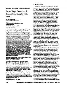
Figure 1. Radar signal concept.
Although the automatic detection/tracking [5]‐[19] and recognition of targets [20]‐[25] has been addressed previously, the problem of automatically identifying objects commonly encountered in a desert border surveillance environment has not been analysed before this study. Since border security remains a key issue in homeland security it is imperative to develop radar systems that can help to optimize the capabilities of the border guards, surveillance operators and command staff assigned to secure this strategic region. Given the lack of sufficient coverage from sensors and cameras, it is especially important to build systems able to detect threats at an acceptable rate without overloading the overall surveillance system with false alarms. The targets used in this research come from one of the following classes: human, truck and low flying Cessna Airplane, hence the research presented in this paper could help to alleviate the problems encountered in this vital national security environment. It is also worth noting that this paper is one of the few existing research works that contributes to the study of radar target classification in distinct travel mediums, in this case land and air. The operation modes used for target detection in a typical radar are described in more detail in the next section. A generic neural network for radar target classification is also discussed in Section II. Finally, in Section III the results of simulating the radar detection of targets commonly encountered in a border surveillance environment and their automatic classification using an artificial neural network are presented. 2. Intelligent radar system Overview 2.1 Radar Target Detection In general, the first basic operation of radar is to transmit an RF signals that is analysed and processed to obtain the range, velocity and direction of the target. The radar is capable of detecting, locating and identifying moving targets such as a person, vehicle, etc. [26]. The radar has four modes of operation: 1) initial target detection and estimation, 2) Doppler, 3) high resolution and 4) inverse
2
Int J Adv Robotic Sy, 2012, Vol. 9, 177:2012
synthetic aperture radar. The radar must be adjusted from one mode to the next in order to obtain the final high‐resolution images that will be used by the neural network for recognition purposes. First Mode 1 should be chosen to detect an object in the environment. Once a target has been detected, it is desirable to track its velocity. The radial speed of the target can be directly estimated in Mode 2 using the Doppler principle, which states that the speed of a moving object will affect the frequency of the return signal. After determining the target’s velocity by measuring the Doppler shift of the reflected signal, the system should change to Mode 3 or Mode 4 depending on the velocity output. Mode 3 can provide a high‐resolution range profile as a one‐dimensional signature of the target of interest, while Mode 4 is an imaging technology that can provide a high‐resolution two‐dimensional image of the target. In this research it is assumed that the targets are moving at speeds which allow using Mode 4, hence Mode 3 is not described in this manuscript. The operating modes used in this research are described in more detail next. 2.2 Initial Target Detection and Estimation (Mode 1) The most fundamental problem in radar is detection of a target. This requires determining whether the receiver output is an echo from a reflecting target or only noise. This mode uses the moving target indicator principles to detect the targets of interest. The moving target indicator can distinguish between slowly moving or stationary targets and fast moving targets. For this research, target detection is accomplished by the radar receiver employing an envelope detector followed by a threshold decision to detect the presence of a target. The input signal to the receiver is composed of the radar signal to be detected, and additive zero‐means white Gaussian noise, the return signal is describe in (1). r (t ) s (t ) n(t ) (1)
where s(t)=sin(ω0t) is the transmitted signal, ω0=2πf0, f0 is the frequency and n(t) is the zero‐means white Gaussian noise. Target detection is based on two hypotheses, either the target is present or it is not [27]. In other words, a target is detected when r(t) exceeds the threshold value, vT. The two decision hypotheses are H 0 : r (t ) n(t ) No target detected
H 1 : r (t ) s(t ) n(t ) Target detected (2)
where H0 is hypothesis zero, no target is present, only noise, and H1 is hypothesis one, for which a target is www.intechopen.com
present with noise. The Neyman‐Pearson criterion is used to derive the decision rule as described in [27]. The receiver should choose the correct hypothesis with high probability. The objective is to maximize the probability that a target is detected in the presence of noise, while minimizing the probability that a receiver mistakenly declares a target present when only noise is present. To maximize the probability that the receiver will detect a target in the presence of noise is known as the probability of detection and is defined in (3).
where n(t) is the zero‐means white Gaussian noise, σ is the attenuation factor and D is the time delay in which the signal travel from the transmitter to the target and back to the receiver. A common method of calculating the time delay is to compute the cross‐correlation function of the received signal with the transmitted signal as shown in (8).
Rrs ( ) r (t )r * (t )dt (8)
To find the range of the target, equation (9) is used
Pd P( D0 | H1 ) p1 (r )dr (3) VT
To minimize the probability that the receiver will miss, declaring a target present when only noise is present, is to minimize the probability of false alarm, which is defined in (4) and can be expressed in terms of the Neyman‐Pearson threshold.
Pfa P( D1 | H 0 ) p0 (r )dr (4) VT
These two conditional probabilities are related to each other. Expressing these quantities in terms of the decision region and the likelihood function one can determine the decision rule.
H1 p (r ) (5) Vn 1 VT p0 ( r ) H0
where p0 and p1 represent the prior probabilities for the data given hypotheses 0 and 1, and VT is the threshold value. It is important to know that increasing Pd by lowering the detection threshold results in an increase in the Pfa. The desire to maximize Pd to improve performance will be accomplished by using a likelihood ratio test. The transmitter sends a transmitted signal, hits the target and is reflected back with a time delay , as shown in Figure 1. If a target is detected, the range of the target it determined by estimating the time delay between the transmitted s(t) and the returned signal r(t). The signals are describe in equation (6) and (7). s(t ) sin(2f 0t ) (6)
r (t ) * sin(2f 0 (t D)) n(t ) (7)
www.intechopen.com
R
c 2
(9)
where R is the target’s range, c is the speed of light, c= 3*108 m/s, and τ is the delay. The factor of ½ is needed to account for the two‐way time delay. For range processing, the return signal must first be filtered in order to reduce the effects of noise that get into the signal. A proper filter to use on the signal is a “matched filter” to the original signal. To get the range, it is necessary to know the time that elapsed between sending the signal and receiving the return signal. The distance to the target can be determined by using equation (9). 2.3 Doppler (Mode 2) The radial speed of the target can be measured directly using the Doppler principle, which states that the speed of a moving object will affect the frequency of the return signal. The Doppler frequency determines the target radial velocity and can distinguish between moving and stationary targets [26]. If the target happens to be moving, the reflected signal will have a different frequency from the one that was transmitted. The difference between these frequencies is referred to as a Doppler shift. The Doppler shift can be positive or negative depending on whether the target is coming toward or is moving away from the radar. If the signal bounces off the target and if the object is moving towards the radar, then the signal is compressed and the frequency is shifted up. If the target is moving away from the radar, then the frequency is shifted down. A typical signal for this mode is a series of pulses as the transmitted signal. The series of pulses hits the target and is reflected back with a Doppler shift on the return signal. The returned signal is then multiplied by a complex exponential with a certain phase. The reflected signal is of the form
r (t ) s(t 0 )e j 2f d ( t 0 ) (10) where fd the Doppler is shift and τ0 is the delay associated with the target. Janette C. Briones, Benjamin Flores and Raul Cruz-Cano: Multi-Mode Radar Target Detection and Recognition Using Neural Networks
3
In order to detect the frequency shift between the transmitted signal and the received signal, the Fourier Transform (FT) of both the transmitted and received signals is obtained, and the analysis of the spectrum of the two signals is performed. The shift of the spectrum shows the Doppler shift. To calculate the velocity given the Doppler shift, the carrier frequency of the radar and the speed of light is calculated by:
fd
2v f c (11) c
where fd is the Doppler shift, v is the target radial velocity, c is the speed of light and fc is the carrier frequency. Equation (12) is used when there is an angle between the radar line of sight and the target, for this equation, 2vcosθ, is the radial velocity and θ is the total angle.
fd
2v cos (12)
Having established the target detection and range, the velocity needs to be obtained. The velocity processing is determined by means of measuring the change in frequency if the target is moving. This shift in frequency is known as the “Doppler shift” [26]. From the Doppler shift in frequency, the velocity of the target can be found by (12). Unless the target is moving at an extremely high speed relative to the speed of light, the Doppler shift will be small and very difficult to detect from one pulse. The solution to this is to transmit a signal containing repeated pulses, therefore, a series of pulses is needed to measure the Doppler shift. Once the target’s velocity is obtained by measuring the Doppler shift of the reflected signal, the system can intelligently change the mode of operations depending on the velocity output. It can go to the next mode of operation, which is the high resolution, or get the Inverse Synthetic Aperture Radar (ISAR) immediately depending how fast the target is moving. 2.4 Inverse Synthetic Aperture Radar (Mode 4) Inverse Synthetic Aperture Radar (ISAR) is an imaging technology that is used to obtain high‐resolution 2‐D images [26] using advanced signal processing techniques, to give a detailed image of the target. ISAR is basically an edition of SAR that can be used to provide images of targets like aircraft. ISAR processing techniques are used for this mode because of its advantages when it comes to imaging targets at high resolutions. It works by emitting a signal and then recording the strength of the reflected signal. The pulses are emitted at an angle and very little of the signal will be reflected back towards the radar, which corresponds to a darker spot on the scattering image. 4
Int J Adv Robotic Sy, 2012, Vol. 9, 177:2012
CHARACTERISTICS
DESCRIPTION
Value
Detection ranges: Air targets Detection ranges: Land targets
Cessna Pedestrian Vehicle
RCS =10m2 RCS =1 m2 RCS =5 m2
Table 1. Typical characteristics and description of the three targets.
The image generation and processing is performed using MATLAB scripts. The simplest way to implement a target model is to represent it as a collection of point scatterers. Each scatterer, therefore, will be characterized by a distance from the radar and by the strength of reflection. The Radar Cross Section (RCS) is enhanced by a larger number of point scatterers and is dependent upon aspect angle to radar. Mode 4 uses a stepped frequency waveform of M burst and each burst is in the form of N stepped frequency pulses to form a matrix of pulses. To find the frequency of the nth pulse in a burst, the following equation was used
f n f o nf (13)
where fo is the initial frequency in a burst and Δf is the frequency step between pulses. Range resolution is a metric that describes the radar system’s ability to detect target in close proximity to each other as a different target [26] and is defined as
r
c 2B
(14)
If we consider N pulses stepped frequency by f, the slant range resolution is define by equation (15)
r
c (15) 2(N 1)f
The Doppler resolution is approximately 1/T where T is the integration time, thus we can conclude the cross range resolution to be
rc
cfd 2w c f c 2w c T
(16)
This equation can help us to form an image by simulation. The matrix of the form m x n dimension represents the range‐Doppler which in turn can be the ISAR image of the objects. To form the image we consider the transfer function to be the sum of the hot spot steady state responses:
n
H AL e i2fTL (17) 1
where TL =2RL/c, AL=1 and H is the sum of phasors. www.intechopen.com
By obtaining the Inverse Discrete FT (IDFT), the target’s reflectivity is obtained as a function of time. Using the IDFT will give the RCS of the scatterer and its location. Table 1 describes typical characteristics and descriptions of the three targets. A parametric representation of the target outline is used as a feature set for classifying the targets. The IDFT of the matrix H(k,j) is taken for each row. After the IDFT, the discrete Fourier transform DFT is computed for each column of N 1
h(k,n) H(k, j)e i2f / N
(18)
j 1
The output images will be represented by D(m,n) and is of the form
D(m,n)
M 1
h(k,n)e
i2m / M
(19)
The ISAR technique will generate a 2‐D high‐resolution image of a target. The matrix obtained will then be used in the neural network to classify the targets. Although the research presented in this manuscript includes different radar operation modes, it does not explore how to automatically switch among them to accomplish the detection and classification of the targets. This problem will be addressed in future research by using fuzzy logic to model the rules necessary to perform these complex decisions in an intelligent manner. Fuzzy logic has proved to be an efficient tool in problems that also have to deal with decision‐making for classification problems [28]‐[30], hence it seems to be a promising approach. 2.5 Target Recognition Using Neural Networks The objective of cognitive radar in this paper is to provide the intelligent system with the capability to not only detect, but also to recognize and classify targets in the appropriate class. The application in this research is surveillance radar that is capable of detecting the different targets listed in Table 1: walking humans, ground vehicles and Cessna aircraft.
Figure 2. Neural network classification model.
www.intechopen.com
Symbol
Description
Value
A Fs fo N t
Amplitude Sampling Frequency Carrier Frequency Number of samples Sampling period Delay
1 V 1000Hz 50Hz 1024 0.001 2 sec
Table 2. Radar System Parameters
The classification of the targets will be performed using a neural network trained with high‐resolution images of these classes. The automatic recognition can be implemented using neural networks because they have proved to be able to correctly classify objects based on noisy images [20]‐[21]. Moreover, there are multiple examples in which neural networks have played an integral part in controlling complex electromechanical systems [31]‐[35]. A neural network is defined as an interconnected group of artificial neurons that uses a computational model for information processing and performs useful computation through a process of learning to obtain knowledge [36]. The knowledge obtained is stored using interneuron connection strength, commonly known as synaptic weights. A learning algorithm is a function that modifies the synaptic weight of the network in an orderly fashion and is used to perform the learning process and to obtain a desired design objective. Once the optimal operation mode has been determined, its parameters are fed into a neural network which determines the type of object being detected by the radar. The output of the kth neuron is defined by
yk ( j 0 wkj x j ) (20) p
where φ is the transfer function, are the input signals, are the synaptic weights of neuron k. The model of a neural network to classify the targets included in this research is shown in Figure 2. This model is based on a feed‐forward neural network that consists of a single hidden layer with 60 neurons in the hidden layer, with a tangent sigmoid as the transfer function and a linear function in the output layer. The input vectors consisted of 2‐D images of the Cessna, truck and human targets, which are transformed into a one‐dimensional vector before being presented to the neural network. There is only one target value associated with each input vector. The target output is the corresponding classification of the target shown in the 2‐D image. A more detailed description of the approach followed to design, train and test the neural network is included in Section III B. Janette C. Briones, Benjamin Flores and Raul Cruz-Cano: Multi-Mode Radar Target Detection and Recognition Using Neural Networks
5
Target\# of Hidden Neurons Truck (0) Plane (1) Pedestrian (2) Overall
50 91% 97% 58% 82%
55 97% 94% 58% 83%
60 94% 97% 94% 95%
65 100% 90% 80% 90%
Table 3. Percentage of correct classification for different numbers of hidden neurons for each of the target classes for the training set.
Figure 3. Cross‐correlation Rrs(τ).
3. Results 3.1 Radar Target Detection Simulation and Results It is assumed that the walking human and the ground vehicle are in the radar line of sight, while the air target, Cessna, is about 5 miles outside. It is also assumed that 20dB SNR is a reasonable detection threshold. The human and the vehicle have the maximum Doppler frequency, since the targets are in the radar’s line of sight. The system uses typical and different waveforms for different modes of operations. As mentioned previously, it is assumed that the operation modes are selected appropriately to perform the target detection task. Table 2 shows the parameters used for the detection radar system simulation. To test the detection of the target, a sinusoidal signal was used as the transmitted signal. The radar return consisted of this signal with a time delay and noise added to the signal. The MATLAB script was run and if a target was detected, the range of the target was determined from the time delay between the transmitted and the returned signal.
For this paper we intended to develop a radar system that operated with a 99% probability of detection and a probability of false alarm of 0.01%. That is the probability that a target was detected in the presence of noise. The probability of false alarm was minimized so that the target is found when noise is present. To achieve the specified performance, the signal to noise ratio (SNR) was obtained. A simulation was performed in MATLAB and a signal was successfully detected using the procedure described next.
The general detection performance of the radar was addressed in the previous section. In this subsection we provide a detailed example of how the detection of a single target is performed. Presenting the complete detection processes for a single target will not only help to clarify Section II’s radar theory, but it will also help to understand how the detection elements produce that information necessary to feed the neural network in charge of classifying the target. Although the results shown in this subsection are for a Cessna airplane, they illustrate the process followed to detect the other types of targets. The reader should keep in mind that that there are many detection techniques and the procedure described in this section is just one of them.
Figure 3 shows the plot of the cross‐correlation between the transmitted and the received signal, and the computed delay for a typical detection. The plot shows the cross‐correlation which is used for obtaining the range information. The cross‐correlation function of the received signal with the transmitted signal is shown in Equation (8).
Figure 5. Cessna image.
Figure 4. Autocorrelation of the signal.
6
Int J Adv Robotic Sy, 2012, Vol. 9, 177:2012
The cross‐correlation allows assessment of the degree of similarity between the signals and identifying the radar return signal in heavy noise. The large peak in the cross‐correlation function indicates that the target detection simulation has been successful and the radar has recognized the presence of a target. The position of the peak carries information about the range for the target. www.intechopen.com
NN Classification\ Actual Class Truck Plane Pedestrian
Truck 83% 17% 0%
Plane 29% 71% 0%
Pedestrian 14% 0% 86%
Table 4. Classification for each of the target classes for the test sets.
The autocorrelation of the signal can be obtained by doing the inverse Fourier transform of the power spectral density of the return signal. The spectral was obtained by performing the discrete time Fourier transforms on the spectra average time autocorrelation of the signal realizations. This formula for the autocorrelation is equivalent to dividing a single signal realization into independent segments correlating each segment and averaging the correlation bin by bin, which was the process used in this research. The autocorrelation of the return signal is shown in Figure 4. It can be observed that the autocorrelation has one peak, proving once again that the simulation of the radar was successful and a target has been detected. Two features were required for high range resolution: 1) the autocorrelation of the frequency modulated signal had to have a spike at the origin similar to Figure 4 and 2) the side lobes of the autocorrelation needed to be shallow and die out with increase time lag. To obtain the range profile, matched filtering of the returned signal, using a simulated version of the transmitted pulse, was performed. The inverse synthetic aperture radar provides high‐resolution maps of remote targets like a terrain. ISAR was used to provide target images, like those of aircraft or ground vehicles. In order to simulate the Cessna, an equation was established for the range of each hotspot. We used 18 hotspots as shown in Figure 5 in order to visualize the Cessna by adding the distance between each hotspot to the reference point. A 2‐D image provided by the ISAR for a Cessna airplane is shown in Figure 6.
3.2 Target Recognition Using Neural Networks Once the target has been detected using the information provided in Figures 3 to Figure 6, a neural network was implemented in MATLAB to classify the objects based on the ISAR’s 2‐D image. Each figure is represented by a 60 by 60 matrix in which each of the 3600 input values represent the range profiles. The dataset used for the training and testing of the neural network consisted of 40 images for each of the three types of objects. Each image has a different signal‐to‐noise‐ratio for the returning signal. For each of the three classes 17.5% of the dataset was reserved for testing. The network used the Levenberg‐Marquardt algorithm [37] for training due to its superior speed and performance compared to the classic back‐propagation algorithm. MATLAB’s Neural Network toolbox includes these training algorithms and hence is was unnecessary to develop custom programs that implement them. To find the optimal number of hidden neurons for the neural network, an exhaustive search was performed over a wide range of possible values. Although preliminary experiments include as few as two or five neurons, and as much as 100 hidden neurons, it was fairly clear that the best performance was obtained by setting the number of hidden neurons in the range shown in Table 3. Given the results presented in this table it was decided to use 60 hidden neurons for the test set. The classification performance for the different types of targets is shown in Table 4. The percentages of correct classifications are in bold. A direct comparison with the correct classification rates provided using other methods (Table 5) is not possible given that this is the first time that this set of targets has been used. Both land targets can be correctly identified more than 80% of the time, which is a performance similar to those listed for other works that deal exclusively with land targets [23]‐[25]. Another set of desirable characteristics of the neural network produced for this research is that vehicles are never mistaken for pedestrians and pedestrians can only be mistaken for other land targets. Target Commercial aircraft [22] Tanks [25] Pedestrians, animals, tracked or wheeled vehicles and clutter [24] Military vehicles [23] Border surveillance Pedestrians, planes and boats [26] Pedestrians, wheeled and tracked vehicles (human performance) [24]
Figure 6. Cessna 2‐D image.
www.intechopen.com
Performance 96%‐98% 96% 88%‐96% 88%‐91% 80% 67% 39%
Table 5. Comparison of performances with other automatic radar recognition systems.
Janette C. Briones, Benjamin Flores and Raul Cruz-Cano: Multi-Mode Radar Target Detection and Recognition Using Neural Networks
7
More importantly, the overall performance is far superior to the human performance mentioned in [24] and to the performance reported in [26], which is the only other work that includes a combination of objects that operate in land and air. These results show that this paper not only presents an original contribution (addressing the border surveillance environment for the first time), but also that the approach selected and its implementation compare well against others works in the research area of radar target classification. 4. Summary A radar system for sending and receiving signals reflected from objects commonly encountered in a border surveillance environment (Cessna airplanes, trucks and pedestrians) was simulated in MATLAB. The returning signals contained noise making the detection and identification of the target difficult. The cross‐correlation of the returned signal was accurately calculated providing the information necessary to asses if the target was successfully detected. The spectrum of the autocorrelation of the signal was also obtained and then used by the ISAR technique to obtain 2‐D high‐resolution images of three different types of targets relevant in border surveillance. The target classification of the images was implemented using neural networks trained using the Levenberg‐Marquardt algorithm. The classification rates were better than those reported for human operators, proving the potential of the proposed approach to alleviate the problems caused by the unreliability of manned radar systems. Before proceeding to the next step, more analysis and comparison of neural network architectures and training methods must be performed in order to discover the optimal method for target classification in this border surveillance environment. In the future, the elements required for a complete and fully automatic cognitive radar will be created and integrated as part of the first author’s dissertation work. 5. References [1] Gini F, Rangaswamy M, (2006) Knowledge Based Radar Detection Tracking and Classification, A John Wiley & Sons, Inc. pp. 9‐29. [2] Haykin S, (2005) Cognitive radar: A way to the future. IEEE Signal Processing Magazine. m. 23:30‐41. [3] Haykin S, (2005) Cognitive Radar Networks. IEEE Journal of Quantum Electronics. j.24. no. 2. [4] Haykin S, (2007) Cognitive Dynamic Systems. IEEE International conference on Acoustics, Speech and Signal Processing. vol. 4, pp. IV‐1369 ‐ IV‐1372, Honolulu, HI
8
Int J Adv Robotic Sy, 2012, Vol. 9, 177:2012
[5] De Maio A, Farina A, and Foglia G, (2007) Design and experimental validation of knowledge‐based constant false alarm rate detectors. IET Radar, Sonar and Navigation. vol 1, issue 4. [6] Romero R and Goodman N.A, (2008) Information‐theoretic matched waveform in signal dependent interference. . IEEE Radar Conference, 2008, pp. 1 – 6, Rome, Italy [7] Butler T.B and Goodman N.A, (2008) Multistatic target classification with adaptive waveforms. IEEE Radar Conferences, pp. 1 – 6, Rome, Italy [8] Zhou F, Zhou D, and Yu G, (2008) Target Tracking in Interference Environments Reinforcement Learning and Design for Cognitive Radar Soft Processing. Congress on Image and Signal Processing. vol. 4, pp. 73 – 77, Sanya, China. [9] Haykin S, Yanbo X, and Davidson T.N, (2008) Optimal waveform design for cognitive radar. 42nd Asilomar Conference on Signals. Systems and Computers, pp. 3 – 7, Pacific Grove, CA. [10] Wang B, Wang J, Li J, (2008) ADP‐Based Optimal Adaptive Waveform Selection in Cognitive Radar. IEEE International Symposium on Intelligent Information Technology Application Workshops, pp. 788 – 790, Shanghai, China. [11] Inggs M, (2009) Passive Coherent Location as Cognitive Radar. International Waveform Diversity and Design Conference, pp. 229 – 233, Kissimmee, FL. [12] Wang B, Wang J, Song X and Han Y, (2009) Optimal Adaptive Waveform Selection Based on ADP in Cognitive Radar. World Congress on Computer Science and Information Engineering. vol. 5, pp. 332‐334, Washington, DC. [13] Wei Y, Meng H, and Wang X, (2009) Adaptive single‐tone waveform design for target recognition in cognitive radar. IET International Radar Conference, vol. 2009, issue CP551, pp.707, Guilin, China. [14] Jiu B., Liu H.W, and Wu S.J, (2009) A method of waveform design based on multi‐eigenvector selection. IET International Radar Conference, vol. 2009, issue CP551, pp.608, Guilin, China [15] Bin Wang B, Wang J, Song X, and Han Y (2009) Temporal difference learning waveform selection. ISECS International Colloquium on Computing, Communication,. Control and Management, vol. 4, pp. 533 – 536, Sanya, China [16] Romero R.A and Goodman N.A, (2009) Waveform design in signal‐dependent interference and application to target recognition with multiple transmissions. IET Radar, Sonar and Navigation, vol.3. issue 4, pp. 328 – 340, [17] Wang B, Wang J, Song X, Han Y, and Liu L, (2009) An Improved Algorithm for Waveform Scheduling. 2nd International Conference on Intelligent Computation Technology and Automation,. vol.1, pp. 541 – 544, Changsha, China.
www.intechopen.com
[18] Fan L, Wang J, and Wang B, (2009) Time Allocation in Cognitive Radar for Multiple Target Detection. 3rd International Symposium on Intelligent Information Technology Application. vol. 2, 169 – 172, Nanchang, China. [19] Wang B, Wang J, Song X, and Han Y, (2009) A New Waveform Design Method for Cognitive Radar”. 3rd International Symposium on Intelligent Information Technology Application. vol. 2, pp. 176 – 179, Nanchang, China. [20] Rogers S.K, Colombi J.M, Martin C.E, Gainey J.C, Fielding K.H, Burns T.J, Ruck D.W, Kabrisky M, Oxley M, (1995) Neural networks for automatic target recognition, Neural Networks, vol. 8, Issues 7–8, 1995, pp. 1153–1184. [21] Roth M.W (1990) Survey of neural network technology for automatic target recognition, Neural Networks, IEEE Transactions on , vol.1, no.1, pp.28‐43, Mar 1990. [22] Zyweck A, Bogner R.E, (1996) Radar target classification of commercial aircraft, Aerospace and Electronic Systems, IEEE Transactions on , vol.32, no.2, pp.598‐606, April 1996 [23] Alaee M, Amindavar H, (2008) Chirplet‐based target recognition using RADAR technology, 5th IEEE Sensor Array and Multichannel Signal Processing Workshop, vol., no., pp.451‐454, Darmstadt, Germany. [24] Bilik I, Tabrikian J, Cohen A, (2006) GMM‐based target classification for ground surveillance, IEEE Transactions on Doppler radar, Aerospace and Electronic Systems, vol.42, no.1, pp. 267‐ 278, Jan. 2006 [25] Li Y, Gong H, (2010) An Effective Method for SAR Automatic Target Recognition, Artificial Intelligence and Computational Intelligence, Lecture Notes in Computer Science, 2010, Volume 6319/2010, 440‐447, DOI: 10.1007/978‐3‐642‐16530‐6_52, [26] Mahafza B.R, (2005) Radar Systems Analysis and Design Using MATLAB. 2nd edition, Chapman & Hall/CRC. [27] Whalen A.D, (1971) Detection of Signals in Noise. Orlando, Academic Press.
www.intechopen.com
[28] Melin P, Castillo O, (2005) Hybrid Intelligent Systems for Pattern Recognition Using Soft Computing ‐ An Evolutionary Approach for Neural Networks and Fuzzy Systems Springer 2005: 1‐256 [29] Mendoza O, Melin P, Castillo O, (2009) Interval type‐2 fuzzy logic and modular neural networks for face recognition applications. Appl. Soft Comput. vol.9, issue 4, pp. 1377‐1387. [30] Melin P, Mendoza O, Castillo O, (2010) An improved method for edge detection based on interval type‐2 fuzzy logic. Expert Syst. Appl. 37(12): 8527‐8535 (2010) [31] Fei J, Ding H, Hou S, Wang S, Xin M, (2012) Robust Adaptive Neural Sliding Mode Approach for Tracking Control of a MEMS Triaxial Gyroscope, International Journal of Advanced Robotic Systems, vol. 9, issue 24.. [32] Qiu‐Bo Z, Song‐Hao P, and Chao G, (2010) Motion Planning for Humanoid Robot Based on Hybrid Evolutionary Algorithm, International Journal of Advanced Robotic Systems, vol. 7, No. 3, pp. 209‐216. [33] Gutierrez A, Tuci E and Campo A, (2009) Evolution of Neuro‐Controllers for Robotsʹ Alignment using Local Communication, International Journal of Advanced Robotic Systems, International Journal of Advanced Robotic Systems, vol. 6, No. 1, pp. 25‐34 [34] Chatchanayuenyong T and Parnichkun M, (2008). Time Optimal Hybrid Sliding Mode‐PI Control for an Autonomous Underwater Robot, International Journal of Advanced Robotic Systems, vol. 5, No. 1, pp. 91‐98 [35] Shafiei S.E and Soltanpour M.R, (2009). Robust Neural Network Control of Electrically Driven Robot Manipulator using Backstepping Approach, International Journal of Advanced Robotic Systems, vol. 6, No. 4, pp. 285‐292 [36] Haykin S, (1994) Neural Networks A Comprehensive Foundation. IEEE Press. Macmillian College Publishing Company, Inc. [37] Hagan M.T, Menhaj M.B, (1994) Training Feedforward neural networks with the Marquardt Algorithm. IEEE Transaction on Neural Networks, vol. 5, issue 6, pp.989‐993.
Janette C. Briones, Benjamin Flores and Raul Cruz-Cano: Multi-Mode Radar Target Detection and Recognition Using Neural Networks
9