Multi-objective aggregate production planning model with fuzzy ...

Life Science Journal 2013;10(4)

http://www.lifesciencesite.com

Multi-objective aggregate production planning model with fuzzy parameters and its solving methods Navid Mortezaei, Norzima Zulkifli, Tang Sai Hong, Rosnah Mohd Yusuff Department of Mechanical and manufacturing Engineering, Universiti Putra Malaysia, Serdang 43400, Malaysia [email protected] Abstract: Aggregate production planning (APP) is considered as mid-term decision planning. The purpose of multiperiod APP is to set up overall production levels for each product category to meet fluctuating or uncertain demand in the near future and to set up decisions and policies on the subject of hiring, lay-offs, overtime, backorder, subcontracting, facilities and inventory. In this study, we develop a new multi-objective linear programming model for general APP for multi-period and multi-product problems. We assume that, there is uncertainty in critical input data (i.e., market demands and unit costs). This model is suitable for 24-hour production systems. To show practicality of our model, we will implement this model in a case study. Finally, we propose an interactive solution procedure for achieving the best compromise solution. [Navid Mortezaei, Norzima Zulkifli, Tang Sai Hong, Rosnah Mohd Yusuff. Multi-objective aggregate production planning model with fuzzy parameters and its solving methods. Life Sci J 2013;10(4): 2406-2414] (ISSN:10978135). http://www.lifesciencesite.com. 322 Keywords: fuzzy aggregate production planning; fuzzy AHP; genetic algorithm; TOPSIS used to the task. Then, if that worker is transferred to operate a different task, their skill with the new task would likely be lower than that with the old task. This also impacts productivity. A feasible way to evaluate the extent to which productivity falls is to evaluate training cost and cost due to the loss of production. Therefore, they add to their model cost of transferring workers as a cost parameter. They compared two situations: 1) the worker cannot transfer among production lines, and 2) the worker can transfer between lines. The results of APP model showed that the total cost increases about 5% when the workers did not transfer among production lines; however, the goals and model inputs in these APP models were assumed to be crisp. In the real world, APP problems with deterministic parameters are unsuitable for yielding an effective solution. In the real word, APP problems, input data or parameters such as demand, resources, and costs, are generally imprecise due to incomplete or unobtainable information (Baykasoglu, and Gocken, 2010; Wang, and Liang, 2004). These imprecise parameters can be defined as random numbers with probability distribution, fuzzy numbers or interval numbers (Baykasoglu, and Gocken, 2010). Recently, several researches have been conducted on fuzzy APP. Mula et al. (2006) reviewed more than 87 articles focused on production planning under uncertainty. The results of their study revealed that, most of the analytical models were crisp or mentioned only one type of uncertainty and assumed the simple structure of the production process. Therefore, they suggested that more researches need to be done in the future about production planning under uncertainty. Aliev, et al. (2007) proposed an APP model in a supply chain. In this model, market demand, production capacity and

1. Introduction Aggregate production planning (APP) determines the best way to meet forecast demand in the intermediate future, often from 3 to 18 months ahead, by adjusting regular and overtime production rates, inventory level, labor levels, subcontracting and backorder rates, and other controllable variables. APP aims to identify production, inventory and work force levels to meet fluctuating demand requirements over an intermediate-range planning horizon (Chase and Aquilano 1992). Other forms of family disaggregation plans that are derived from APP are master production schedule, material requirement planning and capacity plan. In this research, we will develop a multiple objective APP model for multiproduct and multi-period. Also, in this model, we will assume that costs and demand and resources are imprecise which have triangular possibility distributions. In this section, we review some pervious researches. Baykasoglu (2001) extended Masud’s (1980) model by adding subcontracting and setup decisions or setup cost of product, setup time of product, and subcontracting cost of product. He developed a multi-objective linear goal programming model that with the following model objectives: 1) maximization of profit, 2) minimization of workforce changes, 3) minimization of inventory investment, and 4) minimization of backorder. To solve the model, he applied Tabu search, due to the high complexity of the model and the large number of model constraints. Techawiboonwong and Yenradee (2003) developed a linear model for multi-product APP that enabled workers to be transferred among production lines. Their model had only one objective function or minimizing total cost. In reality, when a worker performs any task for a long time, they get

2406

Life Science Journal 2013;10(4)

http://www.lifesciencesite.com

storage capacity in production environment were uncertain. They solved their model by using the genetic algorithm to achieve near- optimal solutions. They compared their fuzzy model with crisp and disintegrated approaches. Comparison of the results of fuzzy and crisp integrated production-distribution aggregate planning showed that the profit achieved by the fuzzy model was 5-10% higher than the crisp model, especially, when the actual demand declined from the forecasted value or the capacity plummeted over the planning horizon. Torabi et al. (2009) developed a fuzzy hierarchical production planning comprised of two decision-making levels. Their proposed model attempted to maximize total profit or maximize the difference of the revenue and operation costs. In their model, all cost parameters were imprecise. Their results showed that hierarchical production planning models with fuzzy data are more practical than hierarchical production planning models with crisp data. Other APP models are Fung et al. (2003), Wang et al. (2003), Sillekens et al. (2011). However, the majority of APP models have cost-related objectives, whereas non-cost objectives are often sought by managers. This article is organized as follows: Section 2 introduces the problem and lays the frameworks for problem formulation of multi-objective APP model. Section 3 proposes a procedure for solving fuzzy APP model. Implementation of APP model (case study) is given in Section 4. Finally, Section 5 gives some conclusions and suggestions for further studies.

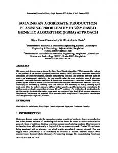
2003). Therefore, forecast demand-related operating costs, and machine and labor capacities are fuzzy over the planning horizon. In this research, we assume that our imprecise input data are triangular positive fuzzy numbers R= (R1, R2, R3) as shown in Figure 1. The membership function is as follows:

µ(x)=

[(x-R2) /(R2-R1)]+1 (R1≤ x ≤ R2), [(x-R2) /(R2-R3)]+1 (R2≤ x ≤ R3) 0 (x≤R1 OR x≥R3)

where x is decision variable (1) Other assumptions are: 1) Average hiring and firing cost are considered; 2) Raw materials are always available without shortage; Appendix 1: Transformation method (Okada et.al 1991, Gen et.al 1992) Suppose we have fuzzy multi-objective model as follows: Max zk= Σ ckj xj, k=1,2,.., q1 Min zk= Σ ckj xj, k=q1+1,.., q=q1+q2 Subject to: Σ aij xj ≤ bi i= 1,2,…,m1 Σ aij xj ≥ bi i= m1+1,…, m2 Σ aij xj = bi i= m2+1,…,m=m1+m2+m3 xj≥0 j= 1,…,n where

2. Fuzzy aggregate production planning model In this section, we develop a new mathematical model for APP problem. The characteristics and assumptions of the model can be described as follows.it is assumed that company produces N types of products to fulfil market demand over planning horizon T. A manufacturer wants to find, for each product and each planning period, the ‘best’ production level and inventory level. It also wants to find the workforce level for each period. The forecasted maximum demands for each product do not necessarily remain constant from period to period. In addition, a portion of the forecasted demand (which can also vary from period to period) must be satisfied in that particular period. The rest of the forecasted demands can either be backordered or not satisfied at all; however, all backorders must be fulfilled within the next period. Assigning a set of crisp values for model parameters is inappropriate for dealing with ambiguous APP decision problems; thus, we assume that environmental coefficients and related parameters are uncertain (Gen et al., 1992; Wang and Liang, 2004; Alive et al., 2007; Torabi et al., 2009; Baykasouglu et al., 2010; Tang et al.,

ckj=(ckj1,ckj2,ckj3) is a fuzzy coefficient of the k-th objective function and j-th decision variable aij =(aij1,aij2,aij3) is a fuzzy technical coefficient of the i-th constraint and j-th decision variable bi =(bi1,bi2,bi3) is a fuzzy available resource of i-th constraint xj is decision variables. All fuzzy parameters in this multi-objective model are triangular fuzzy numbers. Crisp multi-objective linear model can be computed by following formulation: Max zk= Σ [(1-α)ckj3+α ckj2] xj, k=1,2,.., q1 Min zk= Σ [(1-α)ckj1+α ckj2 ]xj, k=q1+1,.., q=q1+q2 Constraint: Σ [(1-α)aij1+α aij2] xj ≤ (1-α)bi3+α bi2,

2407

i= 1,2,…,m1

Life Science Journal 2013;10(4)

http://www.lifesciencesite.com

Σ [(1-α)aij3+α aij2 ]xj ≥ (1-α)bi1+α bi2, i= m1+1,…, m2 Σ [(1-α)aij1+α aij2 ]xj ≤(1-α)bi3+αbi2,

I22 –B22 –I23 +B23+ P23 < 2660000; I22 – B22 – I23 + B23 + P23 > 2620000; I23 – B23- I24 +B24 +P24 < 1940000; I23 – B23 – I24 + B24 + P24 > 1920000; End.

i= m2+1,…,m

Σ [(1-α)aij3+ α aij2 ] xj ≥(1-α)bi1+αbi2, i= m2+1,…,m xj≥0 j= 1,…,n where α is a cutoff value between zero to one, α=[0,0.1,0.2,0.3,…,1]. Appendix 2: A sample of input data (α= 0) for Shahab Shishe company example (max-min method) Max λ λ-((1/189023)*(395587-(0.016p11 + 0.016p12 + 0.016p13 + 0.016p14 + 0.007p21 +0.007p22 +0.007p23 + 0.007p24 + 440w1 +440w2+ 440w3+440w4+ 0.003I11+ 0.003I12+ 0.003I13 + 0.003I14+0.0008I21+ 0.0008I22+ 0.0008I23+ 0.0008I24))) 1600000; P14+ I13-B13 > 1500000; P21 > -4540000; P22+I21-B21> 2650000; P23+I22-B22>2550000; P24+I23-B23> 1880000; 0.018p11+0.013p21- 744w1 < 0; 0.018p12+0.013p22744w2 < 0; 0.018p13+0.013p23- 744w3 < 0; 0.018p14+0.013p24- 744w4 < 0; 0.0002p11+0.00015p21 1580000; P21 – I21 + B21 < -4480000; P21 – I21 + B21 > -4500000; I21 – B21 –I22 + B22 + P22 < 2740000; I21 – B21 –I22 + B22 +P22 > 2700000;

3) Production system cannot operate with less than a certain number of workers (minimum workforce level); 4) Overtime and subcontracting are not allowed.

Figure 1. Triangular fuzzy number R After reviewing the literature and considering practical solutions, the proposed fuzzy APP model selected total cost, changes in work force level, and customer service as objective functions (for total costs, see Gen et al., 1992; Wang and Liang, 2004; Alive et al., 2007; Baykasouglu et al., 2010; Tang et al., 2003; for changes in workforce level, see Gen et al., 1992; Baykasouglu et al., 2010; Masud, 1981; and for customer service, see Chen and Liao, 2003). The three objective multi-period multi-product APP model with fuzzy parameters can be formulated as follows: Indices: n product type t planning period Decision variables: pnt units of production for product n in period t (units) wt work force level in period t (man-day) Int inventory level for product n in period t (units) Bnt backorder level for product n in period t (units) wht worker hired in period t (man-day) wlt worker lay-off in period t (man-day) Parameters and constants: N total number of products T total number of planning periods in the planning horizon cpnt production cost for product n in period t ($/unit) ct labor cost in period t ($/man-period) cint inventory carrying cost for product n in period t ($/unit-period) cht cost to hire one worker in period t ($/man-day) clt cost to lay off one worker in period t ($/manday) csnt cost of stock out product n in period t ($/unitperiod)

2408

Life Science Journal 2013;10(4)

http://www.lifesciencesite.com

Hn hours of labor needed for each unit for product n Unt hours of machine usage per unit of nth product in period t (machine-hour/unite) Rt maximum working hours in period t (a month), equal to regular working hours per worker per day* working shift in per day* working days for period t In0 initial inventory level for product n (units) Bn0 initial backorder level for product n (units) w0 initial work force level (man-day) Dnt forecasted demand for product n in period t (units) Dmin,n minimum demand for product n in period t (units) wmax maximum workforce level available in period t (man-day) wmin minimum workforce level available in period t (man-day) Mt max maximum machine capacity available in period t (machine-hour) cpnt, ct, Dnt, Dmin,n, wmax,Unt and Mt max are triangular fuzzy numbers. Objective functions: (1)Minimize total cost:

3. Solving procedure For solving our fuzzy APP model, the following steps are required: Step 1: Formulate a fuzzy model Step 2: Transform fuzzy model into crisp model by using the transformation method proposed by Okada et al. (1991), (see Appendix 1). Step 3: Solve the crisp multi-objective linear model after setting α (α-cut) parametrically through multiobjective genetic algorithm. Step 4: Determine the weight of each objective function by using fuzzy AHP method proposed by Chang (1996). Step 5: Finding the best compromise solution by using TOPSIS method proposed by Hwang and Masud (1980). 3-1. Fuzzy AHP In this study, we used fuzzy AHP method proposed by Chang (1996) for determining the weight of each objective or minimizing total cost, minimizing the change in workforce level and maximizing customer service. For these purposes, managers of the company evaluated three objectives. As a result of their evaluation, the metrics of pairwise comparison are given in Table 1. Then, we calculated fuzzy synthetic extent by Equation 12. Si= ∑ mgij. [ ∑ ∑ mgij ]-1 (12) where all mgij (j=1,…,m) are triangular fuzzy numbers. mgi1, mgi2,… mgim are values of extent analysis of ith objective for m goals.

N T

min Z1= ∑ ∑ cp~t pnt + ct wt + Int cint

(2)

n=1 t=1

(2) Minimize the changes in work force level: T

min Z2= ∑ ( wht + wlt )

(3) 3-2. Genetic algorithm The genetic algorithm is a powerful method for combinatorial optimization problems. Our implementation of genetic algorithm is presented as follows.

t=1

(3) Maximize customer service: N

T

N

T

max Z3=( 1 - ∑ ∑ Bnt / ∑ ∑ Dnt ) n=1 t=1

(4) 3-2-1. Selection Selection provides the opportunity to deliver the gene of a good solution to the next generation. In this study employs the pareto tournament method proposed by Horn, Nafpliotis and Goldberg in 1994. In this method, two candidates for selection are picked at random from the population. A comparison set of individuals is also picked randomly from population. If one candidate is dominated by comparison set but the other is not dominated, the non-dominated candidate is selected for reproduction. If both candidates are either non-dominated or dominated, a sharing method according to the niche count is used to choose the winner. Candidate with the smaller niche count is selected as the winner. In this research, tournament size is equal 2.

n=1 t=1

The constraints: wmin≤wt ≤ wmax wt= wt-1 + wht – wlt

(5) (6)

N

ΣHn pnt ≤ Rt wt

(7)

n=1

Int – Bnt = In,t-1 – Bn,t-1 +pnt -Dnt

(8)

pnt + In,t-1 – Bn,t-1 ≥ Dmin,n

(9)

N

Σ Unt pnt ≤ Mt max

(10)

n=1

pnt, wt, Int, Bnt,wht, wlt ≥ 0; n=1,…,N; t=1,…,T

(11)

2409

Life Science Journal 2013;10(4)

http://www.lifesciencesite.com

Table 1. Pairwise comparison of three objectives Z1 Z2 Z3 Z1 (1, 1, 1) (3/2, 2, 5/2) (5/2, 3, 7/2) Z2 (2/5, 1/2, 2/3) (1, 1, 1) (2/5, 1, 3/2) Z3 (2/7, 1/3, 2/5) (2/3, 1, 5/2) (1, 1, 1) Where Z1= minimize total cost, Z2=minimize changes in workforce level and Z3= maximization customer service. Degree of possibility of M1 ≥ M2 is calculated by Equation 13. V (M1≥M2) =1 if m1≥m2, V (M2≥M1) = l1-u2/ (m2-u2) – (m1-l1), otherwise (13) When M1= (l1, m1, u1) and M2= (l2, m2, u2) are triangular fuzzy numbers. The results of computation are: s1= (0.35, 0.55, 0.8), s2= (0.12, 0.22, 0.36), and s3= (0.14, 0.21, 0.44); and V (s1≥s2)=1, v (s1≥s3)=1, v (s3≥s2)=1, v (s2≥s1)=0.14, v (s3≥s1)= 0.2, v (s2≥s3)=0.94. Finally the weights of each objective after normalization are W= (0.75, 0.1, 0.15). 3-2-2. Reproduction The best chromosomes that have a lower fitness function are selected for reproduction. 3-2-3. Crossover Scattered crossover is used in this study. Scattered crossover creates binary vectors randomly. It then selects the genes where the binary vector is one from the first parent, and genes where the vector is a zero from the second parent and then combines them to form the child. For example, parent1= [2 3 4 5] and parent2= [1 2 3 4] and the random crossover vector is [11 0 0], and the child will be [2 3 3 4]. 3-2-4. Mutation In our implemented GA, we used adaptive feasible mutation. Adaptive feasible mutation randomly generates directions that are adaptive with respect to the least successful or the unsuccessful generation. 3-2-5 Fitness function The objective functions are chosen as the fitness function that it defined in Section 2. 3-2-6. Termination condition The search process stops if the number of generations exceeds the maximum number of generations, or if some specified number of generations is reached without improving upon the of best-known solution. Solutions or individuals are real decision variables such as production, inventory and backorders. 3-3. TOPSIS Among the many famous multiple-criteria decision-making methods for ranking and selecting numerous possible alternatives through the measuring Euclidean distances, TOPSIS (technique for order performance by similarity to ideal solution) is a practical and useful technique first introduced by Hwang and Yoon (1981).(Goyal et al., 2012). TOPSIS is based on the concept that a chosen alternative should not only be nearest to the positive ideal solution (PIS) but also should be furthest from the negative ideal solution (NIS) (Goyal et al., 2012,

Sajedi et.al, 2013).To determine a compromise solution, we will use TOPSIS method as follows: q

Uj+= ( ∑ Wk (Zk j- ZkB)2 / Zk*2)1/2, K=1

j = 1,..., v

q

(14)

Uj- =( ∑ Wk (Zkj - ZkW)2 / Zk*2)1/2, K=1

j = 1,..., v

(15)

v

Zk* = ( ∑ Zkj2 )1/2 j=1

k= 1, 2,..., v

(16)

ZkB : the best value of k-th objective function ZkW : the worse value of k-th objective function Wk weight of k-th objective function which is obtained in Section 4-1. We obtain the nearest nondominated solution to best value using the following equation. ej* = Uj- / Uj+ + Uj-, 0 < ej* < 1, j = 1, 2,..., v (17) The greater value of ej* will be selected as a compromise solution. 3-4. Multi-objective technique There are several ways to solve multi-objective linear programming models in the literature; among them, the fuzzy programming approaches are more common. Zimmermann (1978) proposed the first fuzzy approach for solving multi-objective linear programming problems, called max–min approach. Max-min is single-phase method which tends to maximize overall satisfaction degree of objective (surrogate objective of λ). In this method, the following formulation is used for solving multiobjective linear problems: Max λ Subject to: λ≤ (zk(x)-zkNIS) /(zkPIS-zkNIS), k=1, …, L λ≤ (wsNIS-ws(x)) / (wsNIS-wsPIS), s=1, …, r,

2410

Life Science Journal 2013;10(4)

http://www.lifesciencesite.com

λ ϵ [0,1], x ϵ X, where k is maximum objectives and s is minimum objectives. The linear membership function of these objective functions can now be computed as follows:

µz1=

1 (z1NIS – z1) / (z1NIS- z1PIS) 0

if z1< z1PIS if z1PIS≤ z1≤ z1NIS if z1> z1NIS

µz2=

1 (z2NIS – z2) / (z2NIS- z2PIS) 0

if z2< z2PIS if z2PIS≤ z2≤ z2NIS if z2> z2NIS

There is a four-period planning horizon of four months based on the Iranian calendar. The model includes two types of product or tubes and bulbs. The forecast demand, minimum demand, production cost, payroll cost, maximum machine capacity and maximum workforce level are fuzzy numbers with triangular possibility distributions from period to period. Table 2-3 summarizes the forecast demand, minimum demand and cost data used by Shahab Shishe Company. Other relevant data are as follows. The hours of labor needed for each unit production are 0.018 for tubes and 0.013 for bulbs. Hours of machine usage for each of four planning periods are (0.0002, 0.00023, 0.00026) and (0.00015, 0.00018, 0.0002) for tubes and bulbs respectively. Maximum machine capacities are (700, 720, 744) for tubes and bulbs in each of the four planning periods. We have 31 working days per period (month), three working shifts of eight hours each, and 24 working hours per day. The initial workforce is 68 workers and the maximum workers allowed are (60, 70, 80) for periods 1 to 4.

1 if z 3> z3PIS NIS PIS NIS µz3= (z3- z3 ) / (z3 – z3 ) if z3PIS≤ z3 ≤ z3NIS 0 if z 3> z3NIS In this research, besides solving our model by multi objective genetic algorithm, we will use max-min formulation to convert multi-objective problem into single-objective problem and then solve this singleobjective problem through the simplex method (exact method). To compare the objective values obtained by LINGO with the results of the multi-objective genetic algorithm, a quality measure, the percent deviation of solution, is defined according to the following equation (Ramezanian et al. 2012): % deviation = (objective function value of GA objective function value LINGO/ objective function value LINGO)*100 (19) 4. Implementation of model (Case study) 4.1. Case description Shahab Shishe Company is used as a case study to demonstrate the practicality of the proposed methodology. Shahab Shishe Company produces two types of products, tubes and bulbs, which are used for producing lamps. The APP decision problem for Shahab Shishe Company is described as follows.

Product Tubes Bulbs

cpnt ($/unit) (0.016, 0.02, 0.024) (0.007, 0.009, 0.011)

Table 2. Forecast demand and minimum demand data Item D1t

D2t

Dmin1 Dmin2

1 (2040000, 2060000, 2080000) (2500000, 2510000, 2520000) (1900000, 1960000, 2060000) (2460000, 2480000, 2500000)

Period 2 (2070000, 2100000, 2130000) (2700000, 2720000, 2740000) (1970000, 1990000, 2010000) (2650000, 2670000, 2700000)

Table 3. Cost data csnt ($/unit) cint ($/unit) ct ($/worker) 0.015 0.003 0.004 0.0008 (440, 465, 480)

Also, the minimum workforce level is 58 workers. Furthermore, the company has 2400000 beginning inventory for tubes and 7000000 for bulbs. 4.2. Results of problem We transformed fuzzy model into crisp model by using the transformation method proposed by Okada et al. (1991) by 11 different α from zero to one. The genetic algorithm was coded in MATLAB R2009 (a), and all tests were conducted on a laptop computer with a core i5-2410m processor 2.3 GHz

cht 30

3 (1700000, 1730000, 1760000) (2620000, 2640000, 2660000) (1600000, 1650000, 1700000) (2550000, 2580000, 2620000)

($/worker)

4 (1580000, 1620000, 1660000) (1920000, 1930000, 1940000) (1500000, 1550000, 1580000) (1880000, 1900000, 1920000)

clt($/worker) 5

with 4 GB of RAM. The results of solving crisp models by using multi objective genetic algorithm and run times (second) are given in Table 4. For this example the population size is equal to 180 and the number of generations is equal to 360. The computational times recorded in table 4 can be considered reasonable times for a problem of this size.

2411

Life Science Journal 2013;10(4)

http://www.lifesciencesite.com strategy results. Optimum solutions for this problem in α=0 are as follows. P1t = [0, 1710000, 1700000, 1500000] or production units for tubes. P2t = [0, 0, 978234, 1721766] or production units for bulbs. Wt = [67, 67, 67, 67] or workforce level in the four periods. I1t = [360000, 0, 0, 0] or inventory level for tubes in four months. I2t = [4500000, 1800000, 158234, 0] or inventory level for bulbs in four months. B1t = [0, 0, 0, 80000] or backorder level for tubes per period. B2t = [0, 0, 0, 40000] or backorder level for bulbs per period. Wht =[0, 0, 0, 0] or workers hired per period. Wlt =[1, 0, 0, 0] or workers laid off per period. Z1 = 221626, Z2 = 1, Z3 = 0.993 Satisfaction degree of each objective function is: µz1=0.92, µz2=0.95 and µz3=0.79. %Deviation between optimum result (max-min) and GA result z1=2.9%. It can be concluded for a problem of this size, that max-min approach is most suitable.

Table 4. Values of objective functions at different levels of α α Z1 Z2 Z3 Run time(s) 0 228172 4 0.981 2 0.1 231673 4 0.981 3 0.2 235232 4 0.982 2 0.3 238710 5 0.982 2 0.4 240878 5 0.982 3 0.5 245792 5 0.982 3 0.6 249984 5 0.984 2 0.7 253076 5 0.984 4 0.8 256213 5 0.983 3 0.9 258046 4 0.986 3 1 276802 4 0.962 3 By using TOPSIS, we can obtain compromise solutions (α = 0) among dominated solutions. The solutions in α = 0 are as follows: P1t = [416666, 1193334, 1700000, 1600000] or production units for tubes P2t = [0, 0, 810000, 1950000] or production units for bulbs Wt = [68, 68, 69, 72] or workforce level in the four periods I1t = [776666, 0, 0, 0] or inventory level for tubes in four months I2t = [4480000, 1740000, 0, 0] or inventory level for bulbs in four months B1t = [0, 100000, 99999, 81104] or backorder level for tubes per period B2t = [0, 0, 70000, 40000] or backorder level for bulbs per period Wht =[0, 0, 1, 3] or workers hired per period Wlt =[0, 0, 0, 0] or workers laid off per period. Z1 = 228172, Z2 = 4, Z3 = 0.981

5. Conclusion In this paper, we formulated aggregate production planning with fuzzy parameters. To transformation a fuzzy APP model into a crisp model, we used the transformation method suggested by Okada et al. (1991). We solved crisp APP models (11 crisp models with 11 different α values ranging from zero to one) by using genetic algorithm. Then, we combined fuzzy AHP and TOPSIS to achieve the best compromise solution. This model is more suitable for 24-hour production systems. We used real-world problems to illustrate the practicality of our model. For further studies, we can extend this model in a supply chain and develop a fuzzy multi-objective production/distribution planning model with some modification of the proposed model.

Now, we compute exact solutions by maxmin method and compare the results. Table 5 shows the total degree of satisfaction of the decision maker (λ) for this example, achieved through max-min method. Table 5. Total degree of satisfaction at different levels of α α λ 0 0.79 0.1 0.73 0.2 0.6 0.3 0.54 0.4 0.58 0.5 0.61 0.6 0.54 0.7 0.59 0.8 0.6 0.9 0.56 1 0.52

Corresponding Author: Mr. Navid Mortezaei Department of Mechanical Engineering, Universiti Putra Malaysia, Serdang 43400, Malaysia [email protected] References 1. Aliev. R. A, Fazlollahi.B, Guirimov. B.G, Aliev. R.R, 2007. Fuzzy-genetic approach to aggregate production-distribution planning in supply chain management. information sciences 177, 4241-4255. 2. Baykasoglu A, 2001. MOAPPS 1.0: aggregate production planning using the multiple objective tabu search. International journal of production research, 29:3, 685–3702.

As demonstrated above, maximum degree of satisfaction is 0.79(for α=0), which confirms our proposed solution

2412

Life Science Journal 2013;10(4)

3.

4.

5.

6.

7.

8.

9.

10.

11.

12.

13.

14.

http://www.lifesciencesite.com

Baykasoglu A, Gocken. T, 2010. Multiobjective aggregate production planning with fuzzy parameters. Journal of advances in engineering software, 41(2010) 1124-1131. Behnamian. J and Fatemi Ghomi.s, 2011. Hybrid flow shop scheduling with machine and resource-dependent processing times. Journal of Applied Mathematical modelling 35 (2011), 1107-1123. Chang.D.Y, 1996. Application of the extent analysis method on fuzzy AHP. European journal of operational research 95(1996) 649655. Chase, R.B. and Aquilano, N.J. 1992. Production & operations management: a life cycle approach. Boston, MA: Richard D. Irwin. Chen, Y.K, Liao, H.C. 2003. An investigation on selection of simplified aggregate production planning strategies using MADM approaches. International Journal of Production Research, 41:14, 3359-3374. Fung. Y. K, Tang. J, Wang. D, 2003. Multi product aggregate production planning with fuzzy demand and fuzzy capacities. IEEE Transactions on systems, man and cyberneticspart A:system and humans, 33(3) 2003, 302313. Gen. M, Tsujimura. Y, Ida. K. 1992. Method for solving multi objective aggregate production planning problem with fuzzy parameters. Journal of computers and industrial engineering 23(1992), 117-120. Goyal, k, Jain, P.K and Jain, M 2012. Optimal configuration selection for reconfigurable manufacturing system using NSGAII and TOPSIS. International journal of production research, 50:15, 4175-4191. Hwang, C.L. and Yoon, K.S., 1981. Multiple attribute decision making: Method and application. New York: Springer. Horn, J., Nafpliotis, N., and Goldberg, DE. A niched pareto genetic algorithm for multiobjective optimization. In: proceeding of first IEEE Conference on Evolutionary computation, 1994, 82-87. Liu, Z, Chua, D and Yeoh, K.W. 2011. Aggregate production planning for shipbuilding with variation-inventory trade-offs. International Journal of Production Research. 49:20, 6249-6272. Masud, A.S.M.and Hwang, C.L., 1980. An aggregate production planning model and application of three multiple objective decision methods. International journal of production research, 18, 741-752.

15. Mula, J, Poler, R, Garcia-sabater, J.P, Lario, F.C, 2006. Models for production planning under uncertainty: A review. International journal of production economics 103:1, 271285. 16. Murata, T, Ishibuchi, H and Tanaka, H, 1996. Multi-objective genetic algorithm and its application to flow shop scheduling journal of computers and industrial engineering.30, 957968. 17. Okada, S.,Y. Nakahara, M. Gen, and K. Ida.1993. A method for transforming multiple objective linear programming problems with trapezoidal fuzzy coefficients. Electronics and Communications in Japan (Part III: Fundamental Electronic Science), 76:10, 73-84. 18. Ramezanian,R, Rahmani,D, and Barzinpour, F, 2012. An aggregate production planning model for two phase production systems: solving with genetic algorithm and tabu search. Expert systems with Applications, 39, 1256-1263. 19. Sajedi, M.A, et.al, 2013. An improved TOPSIS/EFQM methodology for evaluating the performance of organizations. Life Science Journal, 10(1), 4315-4322 20. Sillekens,T, Koberstein, A and Suhl, L. 2011. Aggregate production planning in the automotive industry with special consideration of workforce flexibility, International Journal of Production Research, 49:17, 5055-5078. 21. Tang. J, Fung. Y. K, Yung.K.L, 2003. Fuzzy modelling and simulation for aggregate production planning. International journal of systems science 34:12-13, 2003, 661-673. 22. Techawiboonwong. A, Yenradee.p, 2003. Aggregate production planning with workforce transferring plan for multiple product types. Journal of production planning & control 15(5), 447-458. 23. Torabi. S. A, Ebadian. M, Tanha.R, 2009. Fuzzy hierarchical production planning (with a case study). Journal of fuzzy sets and systems 161(2010),1511-1529. 24. Wang, C.H, Liang, T, F, 2004. Applying possibilistic linear programming to aggregate production planning. International journal of production economics 98 (2005) 328-341. 25. Wang R-C, Liang T-F, 2004. Application of fuzzy multi-objective linear programming to aggregate production planning. Journal of computers and industrial engineering, 2004, 46:17-41. 26. Zimmermann, H.J. Fuzzy programming and linear programming with several objective functions, Fuzzy sets and Systems 1 (1978) 4555.

2413

Life Science Journal 2013;10(4)

http://www.lifesciencesite.com Max λ λ-((1/189023)*(395587-(0.016p11 + 0.016p12 + 0.016p13 + 0.016p14 + 0.007p21 +0.007p22 +0.007p23 + 0.007p24 + 440w1 +440w2+ 440w3+440w4+ 0.003I11+ 0.003I12+ 0.003I13 + 0.003I14+0.0008I21+ 0.0008I22+ 0.0008I23+ 0.0008I24))) 1600000; P14+ I13-B13 > 1500000; P21 > -4540000; P22+I21-B21> 2650000; P23+I22-B22>2550000; P24+I23-B23> 1880000; 0.018p11+0.013p21- 744w1 < 0; 0.018p12+0.013p22744w2 < 0; 0.018p13+0.013p23- 744w3 < 0; 0.018p14+0.013p24- 744w4 < 0; 0.0002p11+0.00015p21 1580000; P21 – I21 + B21 < -4480000; P21 – I21 + B21 > -4500000; I21 – B21 –I22 + B22 + P22 < 2740000; I21 – B21 –I22 + B22 +P22 > 2700000; I22 –B22 –I23 +B23+ P23 < 2660000; I22 – B22 – I23 + B23 + P23 > 2620000; I23 – B23- I24 +B24 +P24 < 1940000; I23 – B23 – I24 + B24 + P24 > 1920000; End.

Appendix 1: Transformation method (Okada et.al 1991, Gen et.al 1992) Suppose we have fuzzy multi-objective model as follows: in all summation symbols (sigma) lower index is j=1 and upper index is n. Max zk= Σ ckj xj, k=1,2,.., q1 n

Min zk= Σ ckj xj, k=q1+1,.., q=q1+q2 J=1

Subject to: Σ aij xj ≤ bi i= 1,2,…,m1 Σ aij xj ≥ bi i= m1+1,…, m2 Σ aij xj = bi i= m2+1,…,m=m1+m2+m3 xj≥0 j= 1,…,n where ckj=(ckj1,ckj2,ckj3) is a fuzzy coefficient of the k-th objective function and j-th decision variable aij =(aij1,aij2,aij3) is a fuzzy technical coefficient of the i-th constraint and j-th decision variable bi =(bi1,bi2,bi3) is a fuzzy available resource of i-th constraint xj is decision variables. All fuzzy parameters in this multi-objective model are triangular fuzzy numbers. Crisp multi-objective linear model can be computed by following formulation: Max zk= Σ [(1-α)ckj3+α ckj2] xj, k=1,2,.., q1 Min zk= Σ [(1-α)ckj1+α ckj2 ]xj, k=q1+1,.., q=q1+q2 Constraint: Σ [(1-α)aij1+α aij2] xj ≤ (1-α)bi3+α bi2,

i= 1,2,…,m1

Σ [(1-α)aij3+α aij2 ]xj ≥ (1-α)bi1+α bi2, i= m1+1,…, m2 Σ [(1-α)aij1+α aij2 ]xj ≤(1-α)bi3+αbi2,

i= m2+1,…,m

Σ [(1-α)aij3+ α aij2 ] xj ≥(1-α)bi1+αbi2, i= m2+1,…,m xj≥0 j= 1,…,n where α is a cutoff value between zero to one, α=[0,0.1,0.2,0.3,…,1]. Appendix 2: A sample of input data (α= 0) for Shahab Shishe company example (max-min method)

11/12/2013

2414