Merkel, Andreas Jung, Thomas Kirchner, and Thomas Brabletz. A transient, EMT- ..... Ortega, Cristina Fernandez Perez, Javier Sastre, Rosario Alfonso, et al.
UNIVERSITY OF TURIN Doctoral School in Life and Health Sciences PhD Program in Complex Systems for Life Sciences
MULTI-OMICS DATA INTEGRATION APPROACHES UNCOVERING CANCER DRIVERS
Candidate: Laura Cantini
Advisors: Prof. Enzo Medico Prof. Michele Caselle
Coordinator: Prof. Federico Bussolino
PHD THESIS Academic years: 2013-2015
2
Abstract Cancer is a complex disease involving progressive accumulation of molecular alterations by neoplastic cells. During the last decade, systematic assessment of these alterations has been carried out through genomic technologies. However, we still have not succeeded in translating this wealth of information into actionable knowledge about disease pathogenesis. This may in part be due to the fact that in most cases each layer of molecular information is studied independently, which impairs detection of complex regulatory interplays. Overcoming this limitation requires integrative analysis of multiple layers of molecular information ("multi-omics"). In this dissertation two such "multi-omics" approaches are proposed to solve specific cancer related problems. Both approaches take advantage of network analysis for systems-level understanding of disease mechanisms. The first methodology integrates microRNA and mRNA expression profiles to detect microRNAs driving colorectal cancer subtypes. The driver role of the identified microRNAs was experimentally confirmed in cell lines. In the second approach, gene networks based on co-expression, proteinprotein interaction, transcription factor co-targeting and microRNA co-targeting are combined into a single multi-network, to extract communities of genes connected by multiple molecular relationships. Many of such communities were found involved in onset and progression of various tumor types. In both cases, information provided by the expression data was further refined through combination either with microRNA expression or with the regulatory layers, which led to identification of cancer related mechanisms that could not be obtained from single "omics" analyses. The results of this work therefore provide evidence of the power of "multi-omics" approaches in extracting knowledge from complex, multidimensional molecular datasets.
Contents List of Figures
7
List of Tables
11
List of Publications
13
Structure of the thesis
15
Introduction 1.1 Control of gene expression . . . . . . . . . . . . . . . . . . . . . . . . . . . . 1.1.1 Transcription Factors: Transcriptional regulation of gene expression 1.1.2 microRNAs: Post-transcriptional regulation of gene expression . . . 1.2 Cancer . . . . . . . . . . . . . . . . . . . . . . . . . . . . . . . . . . . . . . . 1.2.1 Epithelial-Mesenchymal Transition (EMT) . . . . . . . . . . . . . . . 1.3 The "omics" revolution: Sequencing improvements to cancer genetics . . . . 1.4 Networks: powerful tools for "omics" data analysis . . . . . . . . . . . . . . 1.4.1 Networks traditionally studied in biology . . . . . . . . . . . . . . . 1.4.2 Basic network nomenclature . . . . . . . . . . . . . . . . . . . . . . . 1.5 "Multi-omics" data integration . . . . . . . . . . . . . . . . . . . . . . . . .
17 18 18 19 24 25 26 26 27 29 31
I
. . . . . . . . . .
. . . . . . . . . .
. . . . . . . . . .
. . . . . . . . . .
MRNA/microRNA expression data integration
33
2 MRNA/microRNA expression data integration: Background 2.1 CRC molecular subtypes . . . . . . . . . . . . . . . . . . . . . . . 2.1.1 Colon Cancer Subtype (CCS) . . . . . . . . . . . . . . . . 2.1.2 Colorectal Cancer Assigner (CRCA) . . . . . . . . . . . . 2.1.3 Colon Cancer Molecular Subtype (CCMS) . . . . . . . . . 2.2 Analytical approach . . . . . . . . . . . . . . . . . . . . . . . . . 3 MRNA/microRNA expression data integration: Methods 3.1 Dataset assembly and pre-processing . . . . . . . . . . . . . . 3.2 MMRA:Step 1 . . . . . . . . . . . . . . . . . . . . . . . . . . 3.3 MMRA:Step 2 . . . . . . . . . . . . . . . . . . . . . . . . . . 3.4 MMRA:Step 3 . . . . . . . . . . . . . . . . . . . . . . . . . . 3.5 MMRA:Step 4 . . . . . . . . . . . . . . . . . . . . . . . . . .
. . . . .
. . . . .
. . . . .
. . . . .
. . . . .
. . . . .
. . . . .
. . . . .
. . . . .
. . . . .
. . . . .
. . . . .
. . . . .
. . . . .
. . . . .
. . . . .
. . . . .
. . . . .
. . . . .
. . . . .
. . . . .
35 35 35 36 36 37
. . . . .
39 39 41 42 42 44
4
CONTENTS
4 MRNA/microRNA expression data integration: Results 4.1 MMRA applied to MSI vs MSS . . . . . . . . . . . . . . . . . . . . . . . . . . . . . 4.2 MMRA applied to CRC samples subdivided according to the three signatures (CRCA, CCS and CCMS) . . . . . . . . . . . . . . . . . . . . . . . . . . . . . . . . 4.3 Consolidation of microRNA/subtype associations in CRC cell lines . . . . . . . . . 4.3.1 MicroRNA/mRNA cell lines dataset assembly and classification . . . . . . . 4.3.2 Consolidation of microRNA/subtype associations in CRC cell lines: Methods 4.3.3 Consolidation of microRNA/subtype associations in CRC cell lines: Results 4.4 Functional validation of microRNA/subtype associations in CRC cell lines . . . . . 4.4.1 Selection of microRNAs for functional validation . . . . . . . . . . . . . . . 4.4.2 Selection of cell lines for functional validation . . . . . . . . . . . . . . . . . 4.4.3 Detection of mRNA regulation upon microRNA silencing in cell lines . . . . 4.4.4 Pathways modulated in cell lines upon silencing of the various microRNAs . 4.5 Identification of core microRNA predicted targets . . . . . . . . . . . . . . . . . . .
45 45
5 MRNA/microRNA expression data integration: Discussion
59
II
45 50 51 51 51 52 52 52 53 54 54
Multi-network-based integration of different trascriptional data 61
6 Multi-network-based integration of different trascriptional 6.1 Basic multiplex network nomenclature . . . . . . . . . . . . . 6.2 Applications of multiplex networks in biology . . . . . . . . . 6.3 Network community detection . . . . . . . . . . . . . . . . . .
data: Background . . . . . . . . . . . . . . . . . . . . . . . . . . . . . . . . . . . .
7 Multi-network-based integration of different trascriptional 7.1 Construction of the multi-network . . . . . . . . . . . . . . . 7.2 Layers Filtering . . . . . . . . . . . . . . . . . . . . . . . . . . 7.3 Community detection in the multi-network . . . . . . . . . .
data: Methods 71 . . . . . . . . . . . . 71 . . . . . . . . . . . . 73 . . . . . . . . . . . . 74
8 Multi-network-based integration of different trascriptional data: Results 8.1 Multi-network vs. single layer communities: structure and biological significance 8.1.1 Multi-network communities have a small overlap with the communities of the individual layers . . . . . . . . . . . . . . . . . . . . . . . . . . . . . . 8.1.2 Multi-network communities are more informative than those obtained in the expression networks of tumor tissues . . . . . . . . . . . . . . . . . . . 8.1.3 Multi-network communities are enriched in biological components involved in the oncogenic process that one could not get from the expression networks alone . . . . . . . . . . . . . . . . . . . . . . . . . . . . . . . . . . . . . . .
63 63 65 67
77 . 80 . 80 . 80
. 82
9 Multi-network-based integration of different trascriptional data: Discussion 85 9.1 Enriched Chromosomal Locations . . . . . . . . . . . . . . . . . . . . . . . . . . . . 85 9.2 Intersections between Pancreas Ca communities and PCa-related expression signatures . . . . . . . . . . . . . . . . . . . . . . . . . . . . . . . . . . . . . . . . . . . . 89 9.3 Enriched miRNA Regulons . . . . . . . . . . . . . . . . . . . . . . . . . . . . . . . 90 Conclusions and Future Perspectives
91
CONTENTS
Appendices A MMRA validation and comparisons with alternative A.1 Comparison with variants of the pipeline . . . . . . . . A.2 Comparisons with other pipelines and methods . . . . A.3 Pipeline validation in two independent datasets . . . . B Legend figure 8.4
5
93 procedures 95 . . . . . . . . . . . . . . . . 95 . . . . . . . . . . . . . . . . 96 . . . . . . . . . . . . . . . . 98 99
C Acronyms
103
Bibliography
105
6
CONTENTS
List of Figures 1.1
Genetic information flow. In all living cells, the genetic information flows from DNA to mRNA (transcription) and from mRNA to protein (translation).(http://academic. pgcc.edu/~kroberts/Lecture/Chapter\%207/dogma.html) . . . . . . . . . . . . . . . .
1.2
RNA transcription. Overview of the process steps (https://commons.wikimedia.org/ wiki/File:MRNA_(editors_version).svg). . . . . . . . . . . . . . . . . . . . . . . . .
1.3
24
The hallmarks of cancer. The image reports the 10 hallmarks capabilities acquired by cancer cells during neoplastic transformation [1]. . . . . . . . . . . . . . . . . . . . .
1.6
21
Schematic representation of coherent (left) and incoherent (right) feedforward loops. . . . . . . . . . . . . . . . . . . . . . . . . . . . . . . . . . . . . . . . . . . .
1.5
20
RNA translation. Overview of the process steps (https://en.wikipedia.org/wiki/ Translation_(biology)). . . . . . . . . . . . . . . . . . . . . . . . . . . . . . . . . .
1.4
18
25
Comparison of Bayesian networks and ARACNE performances in synthetic gene network reconstruction. (a) Middle panel, the synthetic network, composed of 12 nodes interconneted through black and red arrows representing up-regulation and down-regulation, respectively; Left panel, result of the reverse engineering using Bayesian networks; Right panel, result of the reverse engineering using ARACNE. ARACNE identifies slightly more correct edges than Bayesian networks (13 vs 11) but it also performs substantially better in the assignment of incorrect edges. (b) Sensitivity and precision of ARACNE and Bayesian networks are plotted as a function of the number of samples. The figure was extracted from [2]. . . . . . . . . . . . . . . . . . . . . . . . . . . . . .
2.1
28
Consensus partition that unifies the three classifiers (CCS, CRCA and CCMS). Caleydo view of correspondences between the subtype assignments of 369 TCGA CRC samples by the CCS, CRCA and CCMS classification systems. Edges connecting the subtypes across the different classifiers are colored to highlight overlapping subtypes. Fisher test P values and odds ratios (ORs) of classification overlaps are reported within each edge. The boxes on the right represent a reconciliation of the CRC subtypes defined by the three classifiers into common, larger subgroups. Samples were assigned to a consensus subgroup if at least two of the three classifiers significantly assigned them to a subtype part of the subgroup. INFL, inflammatory; GOB, goblet-like; ENT, enterocyte; STEM, stem-like. The figure was extracted from [3].
3.1
. . . . . . . . . . . . . . . . . . . . . . . 38
Schematic representation of the microRNA Master Regulator Analysis (MMRA) workflow. . . . . . . . . . . . . . . . . . . . . . . . . . . . . . . . . . . . . . . . . .
40
8
LIST OF FIGURES
4.1
Overlap between microRNAs with differential expression across subtypes defined by different classifiers. The Venn diagram shows the numbers of microRNAs differentially expressed in at least one subtype for each of the three classifiers, and the respective overlaps. Most microRNAs were detected as differentially expressed across subtypes in all three classification systems. . . . . . . . . . . . . . . . . . . . . . . . .
4.2
46
Subtypes consensus clustering applied to differentially expressed microRNAs in TCGA dataset. (a) Consensus hierarchical clustering of 14 subtype centroids (CRCA 1 to 5, CCS 1 to 3, CCMS 1 to 6). Each centroid was calculated by averaging, for each of 66 microRNAs differentially expressed in at least one subtype, expression in the samples assigned to the subtype. The dendrogram shows a subdivision of the subtype centroids in three major subgroups: SSM (blue), TA/Enterocyte (red) and Inflammatory/Goblet (green). (b-d) heatmaps displaying the expression of the 66 subtype-specific microRNAs in samples subdivided by, respectively, the CRCA (b), CCMS (c) and CCS (d) classifiers. MicroRNAs are subdivided by fuzzy self-organizing maps in four expression clusters with differential expression across the three consensus subgroups. . . . . . . . . . . . . . . .
4.3
48
CRC subtype signature genes have high mutual information with specific microRNAs. The figure reports GSEA analysis of CRC subtype signatures within selected microRNA regulons, as indicated on top of each panel. The signatures were selected among those enriched in genes contained in the regulon. Within each of the indicated microRNA regulons, genes are sorted by decreasing mutual information with the microRNA, from left to right. The enrichment plots show that the displayed signatures are also enriched in genes with particularly high MI with the microRNA within the regulon. 49
4.4
Transcriptional responses to microRNA down-regulation in CRC cell lines. Radar plots representing transcriptional modulation of functional gene sets during the response of CRC cell lines to down-regulation of, respectively, miR-194, miR-200b, miR203 and miR-429, as indicated. The axes report the GSEA Normalized enrichment scores (NES) for functional gene sets significantly enriched in at least one microRNA downregulation experiment. The grey area indicates a negative NES, meaning that the gene set is down-regulated by microRNA silencing, while positive NES indicates gene set upregulation by microRNA silencing. . . . . . . . . . . . . . . . . . . . . . . . . . . . . .
4.5
56
MicroRNAs antagonizing the SSM phenotype share mRNA targets. Network of interactions between the four functionally validated microRNAs and their core target mRNAs. The network reports mRNA-microRNA interactions detected both in vitro and in vivo (solid lines) and those detected only in vivo (dashed lines). The mRNA node size is proportional to the number of microRNAs with which it is linked and to the number of solid links. A color code is used to highlight genes involved in relevant pathways or signatures. . . . . . . . . . . . . . . . . . . . . . . . . . . . . . . . . . . . . . . . . .
6.1
58
Example of multiplex network. Example of multiplex network with α = 3 layers (represented in red, green and blue) and 10 nodes. Nodes are the same in all the three layers. Intra-layers links are represented with solid lines, while inter-layer interactions (dashed lines) are from each node to itself in the other layers (http://people.maths.ox. ac.uk/kivela/mln_library/visualizing.html). . . . . . . . . . . . . . . . . . . . . .
64
LIST OF FIGURES
6.2
9
Zachary’s network of karate club members. The nodes of the network correspond to the 34 members of a karate club and the links represent their interactions outside the activities of the club. Squares and circles represent the groups that, after fission of the club, supported the instructor (1) and the president (34), respectively. The figure is taken from [4] . . . . . . . . . . . . . . . . . . . . . . . . . . . . . . . . . . . . . . . . . . .
7.1
Schematic representation of the proposed procedure. The schema reports the data required as initial input, the four analytic steps and the final output. . . . . . . . .
8.1
67
72
Size comparison of communities obtained according to the four community detection algorithms. Histograms of comparison in terms of community size between the four community detection algorithms : OSLOM (black), Infomap (red), Louvain (green), Modularity optimization (yellow). . . . . . . . . . . . . . . . . . . . . . . . . .
8.2
79
Comparison of four community detection algorithms in terms of differentially expressed communities. Four algorithms (Infomap (blue), Louvain (red), Modularity optimization (green) and OSLOM (violet)) were tested in their ability to detect communities differentially expressed in the comparison between tumor and normal tissue. Each dot in the plot represents a community, a darker colour identifies those communities that are also functionally homogeneous. On the y-axis are reported the results of the three differential expression criteria: (a) | meani∈C (log2(f oldchange)i ) |; (b) Student’s t-test p-value; (c) sdi∈C (log2(f oldchange)i ). . . . . . . . . . . . . . . . . . . . . . . . . . . .
8.3
81
Comparison between multi-network and expression networks comparison in revealing (normal vs.
tumor) differentially expressed communities. multi-
network (red) and expression (blue) networks were tested in their ability to reveal differentially expressed communities in the comparison between tumor and normal tissue. Each dot in the plot represents a community, a darker color identifies those communities that are also functionally homogeneous. In the columns we report the results of the three differential expression criteria: | meani∈C (log2(f oldchange)i ) | (Criterion 1); Student’s t-test p-value (Criterion 2); sdi∈C (log2(f oldchange)i ) (Criterion 3). . . . . . . . . . . .
8.4
83
Biological components involved in the oncogenic process enriched in the multinetwork communities that we could not get from the expression network. Radar plots of the reciprocal of the enrichment pvalues for (a) chromosomes, (b) pathways, (c) motifs TF/microRNAs and (d) GO. In each radar plot the results of the enrichment analysis are represented for the four tissues: gastric (blue), lung (red), pancreas (green) and colon (violet). Only the functions with an enrichment p-value lower than 10−5 are represented. Function identifiers instead of function names are reported, in Table B.1-4 of the Appendix B the conversion can be found. . . . . . . . . . . . . . . . . . . . . . .
84
10
LIST OF FIGURES
List of Tables 4.1 4.2
MicroRNAs identified by MMRA with differential expression across CRC subtypes and associated to subtype-specific mRNA signatures. . . 50 microRNA downregulation in CRC cell lines leads to modulation of SSM subtype genes and change in subtype assignment . . . . . . . . . . . . . . . 55
8.1 8.2
Choice of the optimal alpha threshold for the disparity filter. . . . . . . . 78 Comparison of community detection algorithms in terms of functionally homogeneous communities. . . . . . . . . . . . . . . . . . . . . . . . . . . . . . 79
9.1
Intersection of Collisson signature and Pancreatic communities. . . . . . 89
B.1 B.2 B.3 B.4
Pathways. . . . . . . . . . Chromosomal locations. Motifs. . . . . . . . . . . . Gene Ontology (GO). . .
. . . .
. . . .
. . . .
. . . .
. . . .
. . . .
. . . .
. . . .
. . . .
. . . .
. . . .
. . . .
. . . .
. . . .
. . . .
. . . .
. . . .
. . . .
. . . .
. . . .
. . . .
. . . .
. . . .
. . . .
. . . .
. . . .
. . . .
. . . .
. . . .
. . . .
. . . .
99 100 100 101
12
LIST OF TABLES
List of Publications Papers included in the thesis: • Laura Cantini, Claudio Isella, Consalvo Petti, Gabriele Picco, Simone Chiola, Elisa Ficarra, Michele Caselle and Enzo Medico. "MicroRNA-mRNA interactions underlying colorectal cancer molecular subtypes". Nature Communications, 6 (11), 2015. • Laura Cantini, Enzo Medico, Santo Fortunato and Michele Caselle. "Detection of gene communities in multi-networks reveals cancer drivers". Scientific Reports, 5, 2015.
14
List of Publications
Structure of the thesis The thesis is divided into four parts: • Introduction. It gives some insights on molecular biology and gene regulatory networks. The main purpose of this chapter is to make the thesis as self-contained as possible. Thus, readers familiar with these topics can skip this chapter without compromizing the understanding of later material. • Part I: MRNA/microRNA expression data integration. It describes the first original result presented in this thesis, corresponding to the first paper of the previous page. It is structured in four chapters: Background, Methods, Results and Discussion (chapters 2-5). • Part II: Multi-network-based integration of different trascriptional data. It presents the second novel result of this thesis, corresponding to the second paper of the previous page. It is structured in four chapters: Background, Methods, Results and Discussion (chapters 6-9). • Conclusions and Future Perspectives.
The results presented in this thesis have been derived by Laura Cantini within the PhD Program in Complex Systems for Life Science of the University of Turin. Part II has been carried out during Laura Cantini’s visiting period in the BECS department at Aalto Univerity, Finland, under the supervision of prof. Santo Fortunato.
16
Structure of the thesis
Introduction The Cell is the fundamental unit of life. All living cells are composed of three main building blocks: deoxyribonucleic acid (DNA), ribonucleic acid (RNA) and proteins [5, 6]. The relevance of these three biopolymers is due to the fact that they are essential for storing, retrieving and translating hereditary information needed to make and maintain a living organism. • DNA is a double-stranded chain whose subunits are termed nucleotides. All nucleotides are composed of a five-carbon sugar (deoxyribose), a phosphate and a nitrogenous base (Adenine (A), Guanine (G), Thymine (T) and Cytosine (C)). In each DNA strand, nucleotides are joined by covalent bonds that connect the sugar of one nucleotide to the phosphate of the next. The two DNA strands run antiparallel to each other and are held together by hydrogen bonds between the four bases (A with T, and C with G). The information stored in DNA is organized into genes, that nowadays can be defined as "a locatable region of genomic sequence, corresponding to a unit of inheritance, which is associated with regulatory regions, transcribed regions and/or other functional sequence regions" [7]. • RNA, such as DNA, is a biopolymer composed of nucleotides. It differs from DNA for two chemical aspects: (i) its nucleotides are ribonucleotides, i.e. they contain the sugar ribose rather than deoxyribose and (ii) RNA contains the nitrogenous base uracil (U) instead of thymine (T). However, the major difference between DNA and RNA concerns their threedimentional structure. Whereas DNA always occurs in cells as a double-stranded helix, RNA is single-stranded and it can therefore fold up into a particular three-dimentional shape. • Proteins are long chains of units, termed amino acids. Each type of protein is composed of a unique sequence of amino acids, that determines the protein’s three-dimentional structure and as a consequence its function in the cell. Most of a cell’s dry mass is represented by proteins that are fundamental for the majority of the cellular activities. The central dogma of molecular biology [8, 9], illustrated in Figure 1.1, states how the genetic information flows within a cell: from DNA to RNA and finally to protein. In particular, when a cell needs a certain protein, the sequence of the corresponding portion of DNA is first copied into messenger RNA (mRNA), according to a process called transcription. Then, when translation takes place, this mRNA is used as template for the protein synthesis. The transcription and translation processes are extensively described in the next section together with the main regulators of these processes: Transcription Factors (TFs) and microRNAs (miRNAs).
18
Introduction
Figure 1.1: Genetic information flow. In all living cells, the genetic information flows from DNA to mRNA (transcription) and from mRNA to protein (translation).(http://academic.pgcc.edu/ ~kroberts/Lecture/Chapter\%207/dogma.html)
1.1
Control of gene expression
The complete genetic information embodied in the DNA sequence is known as genome. Through transcription and translation, the genome determines the cell’s phenotype, corresponding to its appearance and behavior. However, cells with identical genome may have different phenotypes. This happens, for example, to cells belonging to different tissues. In fact, each cell activates distinct tissue-specific transcriptional programs whereby certain genes are transcribed and others remain silent. These transcriptional programs need to be rapidly adjustable in response to environmental changes or developmental signals. Thus, the mechanisms that a cell can achieve to regulate the production of a protein need to be several and of different kind [10, 11]. Among this huge amount of regulators the main two at the transcriptional and post-transcriptional level are Transcription Factors (TFs) [12] and microRNAs (miRNAs) [13–16], respectively.
1.1.1
Transcription Factors: Transcriptional regulation of gene expression
In eukaryotic cells, transcription is performed by three RNA polymerases: RNA polymerase I [17], RNA polymerase II [18], and RNA polymerase III [19]. The three polymerases are structurally similar, but they transcribe different categories of genes. RNA polymerases I and III transcribe genes encoding transfer RNA, ribosomal RNA, and other small RNAs. RNA polymerase II transcribes all genes that encode for proteins and microRNAs. The transcription process by RNA polymerase II (summarized in Figure 1.2) is described here in detail. When RNA polymerase
1.1 Control of gene expression
19
binds the transcription starting site of a gene, the portion of the DNA double helix corresponding to the gene is unwound and one of the two DNA strands acts as template for the synthesis of an mRNA molecule. The RNA nucleotidic sequence is determined by complementary basepairing between DNA and incoming nucleotides. While elongation approaches the end of the gene, specific proteins read the transcription stop signal encoded in the genome, they recognize the tail of the obtained transcript and they cleave it. The obtained pre-mRNA contains both coding (exon) and noncoding (intron) sequences. Then 3’ polyadenylation, 5’ capping and splicing process, corresponding to introns removal, are performed on the pre-mRNA. The result of these modifications, termed mRNA, is finally exported from the nucleus to the cytoplasm. During transcription, a fundamental role is played by a particular category of proteins termed Transcription Factors (TFs) [12, 20]. TFs bind to either enhancer or promoter regions of the target genes helping the correct positioning of RNA polymerase II. They pull apart one of the two DNA strands to allow the beginning of transcription and they release RNA polymerase from the promoter to start its elongation mode. Transcription factors perform these functions alone or with other proteins in a complex. A single transcription factor has several binding sites in the genome, indeed it can target many genes. As a consequence, a TF alteration can exercise a great power on the phenotype of a cell, altering for example an entire pathway or cellular function. To predict which genes would be affected by a TF malfunctioning is important to determine its targets. The identification of TF-targets interactions is performed nowadays through ChIP-sequencing technology (ChIP-seq). ChIP-seq experiments consist of chromatin immunoprecipitation, followed by high-throughput sequencing of the obtained DNA sequence. The Encyclopedia of DNA Elements (ENCODE) project (http://www.genome.gov/encode/), with the aim of identifying all the functional elements encoded in the human genome, is one of the major repositories of TF-target interactions identified through ChiP-seq experiments [21]. This TF-target database is the one that we used in the second part of this dissertation.
1.1.2
microRNAs: Post-transcriptional regulation of gene expression
Once the transcription process is terminated and an mRNA molecule has been exported in the cytoplasm, translation takes place. During this process the information stored in the mRNA sequence is used for protein synthesis. Since there are only 4 nucleotides (A, T, C, G) and 20 different amino acids, the translation process cannot be performed, as transcription, with a oneto-one correspondence between nucleotides and amino acids. Therefore the mRNA sequence is read in consecutive codons, i.e. groups of three nucleotides. Each codon specifies either one of the twenty existing amino acids or a stop to the translation process. The association between each codon and the corresponding ammino acid is performed by transfer RNAs (tRNAs). During translation, each amino acid is attached to a tRNA. An ammino acid is added to the growing end of the protein if the anticodon on its attached tRNA molecule has a complementary basepairing with the processed codon on the mRNA chain. Given that only one of the tRNA molecules in a cell can basepair with each codon, the codon univocally determines the specific amino acid to be added to the growing polypeptide. The translation process is summarized in Figure 1.3. As detailed above, during translation, mRNA is converted into a specific amino acid sequence.
20
Introduction
Figure 1.2: RNA transcription. Overview of the process steps (https://commons.wikimedia.org/ wiki/File:MRNA_(editors_version).svg).
1.1 Control of gene expression
21
Figure 1.3: RNA translation. Overview of the process steps (https://en.wikipedia.org/wiki/ Translation_(biology)).
22
Introduction
However not all the RNAs are translated into proteins, some of them, termed noncoding RNAs, do not code for any protein. The role of noncoding RNAs in the cell is similar to that of proteins, given that they serve as enzymatic, structural, and regulatory components for a wide variety of processes. Among the noncoding RNAs, there are microRNAs (miRNAs), short (2030 nucleotides) single-stranded RNAs with a relevant role in the translation process [13–16]. These small RNAs constitute one of the more abundant classes of gene-regulatory molecules in animals [22] and they have a key role in several biological processes ranging from development and metabolism to apoptosis and signaling pathways [23]. Most miRNAs are transcribed by RNA polymerase II as long as primary RNA. After transcription, the obtained pri-miRNA contains a 5’ CAP structure and a 3’polyadenylated tail. This pri-miRNA is then processed in the nucleus by the enzyme Drosha forming one or more miRNA precursors (pre-miRNA) [24]. Pre-miRNAs, folded in stemloop structures, are exported into the cytoplasm where are processed by the Dicer enzyme into 22 bp double stranded RNAs. Mature miRNAs are then unwound from miRNA duplexes and incorporated into the RNA-induced silencing complex (RISC). Through the RISC complex, the microRNA binds the target mRNA in a short seven-nucleotide region near the 5’ end of the miRNA (seed) [25], inhibiting the target translation or even catalyzing its destruction. Some features make miRNAs especially useful regulators of gene expression. As for TFs, a single miRNA can regulate a whole set of different mRNAs. Moreover, more than one microRNA can partecipate to the translational reduction of the same mRNA, giving to the cell an high number of possibilities to control mRNA translation. These features that make microRNAs particularly useful for gene expression regulation are also those that make their irregular functioning so dangerous. In the next section a brief overview of the main databases reporting miRNA targets is presented. miRNA targets identification The main databases of microRNA-target interactions are: • miRTarBase [26]: a database reporting experimentally validated microRNA-target interactions (MTIs). The database is constructed according to the following procedure: (i) papers concerning MTIs are collected in the PubMed database; (ii) at least two of the developers review the papers and divide MTIs in supported by strong experimental evidence or less strong experimental evidence. MTIs are viewed as having strong support when they are validated by western blot, qPCR, or reporter assays. Instead, high-throughput miRNA target identification methods, including pSILAC, are considered as less strong experimental evidences. This second class of experiments is considered less strong because it generally proves that the over-expression of a miRNA causes a change in the expression of a set of mRNAs, but it is not possible to asses if this happens through a direct or indirect effect. • doRiNA-PicTar [27]: a database reporting predicted microRNA-target interactions. The prediction is performed according to the following procedure: PicTar 2.0 [28] is used to predict miRNA target sites in 3’ UTRs. All the identified 3’ UTR alignments are scanned for perfect and imperfect seed sequences. Perfect seeds consist of a perfect match in the seven nucleotides starting at position 1 or 2 from the 5’-end of a mature miRNA. Imperfect seeds contain one insertion/deletion or mismatches to the 3’ UTR sequence. All candidate sites are subjected to probabilistic scoring by an Hidden Markov Model (HMM). Finally in humans also species conservation is taken into account.
1.1 Control of gene expression
23
• microRNA.org [29]: a database of predicted MTIs. Target prediction is performed through miRanda [30, 31], an algorithm that computes the optimal sequence complementarity between a set of mature microRNAs and a given mRNA. In particular, a miRNA-target alignment score is computed as the position-dependent weighted sum of match and mismatch scores. In addition, a secondary filter is used based on free energy estimation for the microRNA:mRNA duplexs [32]. Moreover, less-conserved predicted target sites are discarded through the use of PhastCons conservation score, which measures the evolutionary conservation across multiple vertebrates using a phylogenetic hidden Markov model [33]. Sequence conservation is an important filter given that it may represent a strong indication of functional constraints for the microRNA-target interaction. • PITA [34]: a predictive database that takes into account target accessibility through a parameter-free model. The model scores microRNA-target interactions by an energy score, ∆∆G: ∆∆G = ∆Gduplex − ∆Gopen , where, ∆Gduplex is the energy gained by binding of the microRNA to its target and ∆Gopen represents the energy required to make the target region accessible for microRNA binding. ∆Gduplex is computed with a modified version of RNAduplex [35], while ∆Gopen is computed through RNAFold [35]. This model seems to predict validated targets more accurately than existing algorithms and shows that site accessibility is not a random parameter, in fact targets are preferentially positioned in highly accessible regions. • TargetScan [36]: a predictive database that associates an mRNA to a given microRNA based on the presence of conserved 6-8mer sites in the mRNA that match the miRNA seed region. This strategy is motivated by the observation that many mRNAs have evolutionary preserved their paring to the miRNA seed [37–39]. Motif conservation is estimated applying branch-length metric to the phylogenetic tree constructed using 3’ UTRs [40]. 3’UTRs were not considered all together, but they were organized based on conservation rate into 10 equally sized bins. This choice is due to the fact that conservation levels can be influenced by external aspects. Finally, to asses if the identified motifs were conserved because of the microRNA targeting or for many reasons other than that, background effects were taken into account, including GC content, dinucleotide content, the interrelation of miRNA seedmatch types, genome alignment quality, and the local conservation rate. The activity of miRNAs and Transcription Factors (TFs) is often highly coordinated [41, 42]. The simplest interaction pattern that describes their combined effect on a common target is represented by FeedForward Loops (FFLs)[42, 43]. Two main FFL states exist: coherent (see Figure 1.4, left) and incoherent (see Figure 1.4, right). A coherent FFL models the situation in which a miRNA helps the transcriptional repression of a target protein that should not be expressed in a particular cell type, acting as a post-transcriptional failsafe control. In other cases, miRNAs and TFs may cooperatively control the protein level, with the TF that activates gene transcription and the microRNA that has a fine-tuning function, keeping the protein level in the correct functional range, according to an incoherent FFL. The disruption of these FFLs is one of the main mechanisms achieved during cancer formation, which is the main topic of the next section.
24
Introduction
Figure 1.4: Schematic representation of coherent (left) and incoherent (right) feedforward loops.
1.2
Cancer
Cancer is one of the most complex and thoroughly researched diseases. It generally arises in consequence of progressive alterations affecting normal cells in the epithelial tissues (skin, colon, breast, prostate or lung). The multistep process that transforms normal cells into neoplastic could be rationalized by the need of these cells to acquire a succession of capabilities that enable them to become tumorigenic and finally malignant. These alterations, termed hallmarks of cancer, are summarized in the work by Hanahan and colleagues [1]. As reported in Figure 1.5, the hallmarks of cancer comprise: uncontrolled proliferation, evasion of tumour suppression, immune destruction avoidance, enablement of replicative immortality, tumor-promoting inflammation, the acquisition of invasive and metastatic potential, creation of a particular microenvironment containing blood vessels, genomic instability, inhibition of cell death and deregulation of cellular energetics. At the molecular level, cancer understanding requires the identification of those genetic alterations that are involved in the neoplastic transformation and the discovery of those mechanisms through which these alterations give rise to the cancerous cell behavior. Indeed the cancer causative potential of a genetic alteration depends on the gene that is affected by the malfunctioning. Those genes that are cancer-critical can be divided into two broad classes, according to whether the cancer risk arises from their over activation or deactivation. Oncogenes are those genes whose gain-of-function (over-activation) can drive a cell toward cancer. Instead, those genes, whose loss-of-function (deactivation) can contribute to cancer, are called tumor suppressors. Oncogenes are generally genes that actively promote proliferation, some examples are RAS, MYC, ABL and EGFR. Contrary, tumor suppressors can be defined as genes which encode proteins that impede tumor formation. Therefore, tumor suppressors contribute to cancer development through the inactivation of their inhibitory function. Examples of tumor suppressors are RB (retinoblastoma-associated), TP53 and BRCA1/BRCA2. An elevated percentage of oncogenes and tumour suppressors is represented by transcription factors [5]. Also miRNAs are documented to be crucial in cancer onset [44, 45]. This is suggested by the fact that about 50% of annotated human miRNAs are located in fragile chromosomal regions that are prone to mutations during tumor progression [46]. The miRNAs involved in cancer progression are classified in oncomirs and tumor suppressors, if they silence tumorsuppressor or oncogenic protein-coding genes, respectively
1.2 Cancer
25
Figure 1.5: The hallmarks of cancer. The image reports the 10 hallmarks capabilities acquired by cancer cells during neoplastic transformation [1].
. Famous oncomiRs are miR-21, miR-155, miR-17-92 cluster. Tumor suppressor microRNAs are miR-34a, let-7, miR-15a, miR-16. MicroRNAs and TFs have not only a fundamental role in tumor onset and progression, but also in Epithelial-Mesenchymal Transition (EMT), the process associated to the acquisition of a metastatic potential. EMT is, among all the tumor associated processes, the most studied one and for this reason we will describe it more in detail in the next section.
1.2.1
Epithelial-Mesenchymal Transition (EMT)
The acquisition of a metastatic potential by cancer cells involves a multi-step process in which primary tumor cells gain local invasiveness, enter the systemic circulation, translocate, arrest at distal capillaries, extravasate and finally proliferate to form distant secondary tumors [47]. To acquire these capabilities epithelial cancer cells need to undergo a drastic change in their phenotype, known as Epithelial-Mesenchymal Transition (EMT). EMT is characterized by loss of cell polarity, decrease of cell-to-cell adhesion and gaining of migration ability [48, 49]. From a molecular point of view, these effects are the consequence of N-cadherin and vimentin expression in place of E-cadherin (CDH1). Among the transcriptional repressors of CDH1 there are ZEB1 and ZEB2, members of the ZEB family, known to be implicated in EMT, tumorigenesis and metastasis [50–54]. The role of the ZEB family in EMT is generally associated to that of the miR-200 family, whose members (miR-141, miR-200a, miR-200b, miR-200c and miR-429) suppress EMT by inhibiting ZEB1/2 translation [55–60]. In particular, a negative feedback loop between the miR-200 family and ZEB1/2 exists [55, 61, 62], with ZEB1/2 that also controls the expression of the miRNA-200 family members. In this thesis, the role of microRNAs and transcription factors in tumor formation and subtyping
26
Introduction
will be explored. This goal wouldn’t be achievable without the huge amount of data produced by high throughput technologies, for this reason, this will be the topic of the next section.
1.3
The "omics" revolution: Sequencing improvements to cancer genetics
In the past decade, the introduction of sequencing technologies caused a drastic revolution in cancer study and treatment, leading to the discovery of new mechanisms involved in cancer development and new candidates for targeted therapies [63][64]. DNA sequencing started in the 1970s with Sanger’s pioneering works [65, 66]. Later, technological advancements, led to the beginning of the Human Genome Project (HGP), which took place from 1990 to 2003 with the aim of mapping and understanding all the genes of human beings. The HGP revealed the sequence that makes up human DNA, transforming our understanding of how genes work, their numbers, their interaction with each other, mutations and many other factors, including our evolutional origins. The main finding was that less than 2% of the genome (20000 genes far fewer than the 80000 − 100000 previously predicted) actually codes for proteins. As a consequence, the vast majority of the genome is composed of non-coding DNA, that is essential for the regulation and expression of the coding regions. A consequence of the HGP completion was a shift in DNA study from one single gene or a small set to an ensemble of genes simultaneously. It is for this reason that the HGP is considered as the starting point of a new era characterized by a data-driven, large-scale engineering program, known as "Omics Revolution" [67, 68]. In recent years, thanks to the introduction of new platforms able to sequence faster and cheaper, a sheer volume of data was made available to scientists. This huge amount of data allowed researchers to simultaneously observe the behavior of a large number of distinct molecular species, leading to the awareness that cancer is the result of a complex interaction among various molecular and cellular components and that, even with full understanding of the individual constituents alone it would not be possible to capture the so called "emergent properties", that can be predicted only analyzing the complete set of molecular constituents as a whole [69–72]. As a consequence, a new research area called systems biology arose [73]. The term "systems biology" was first introduced in 1948 by Norbert Wiener [74], but its application at that time was limited by the inadequacy of the available data. The aim of systems biology is integrating experimental data with mathematical modeling tools to analyze and predict the behavior of biological systems [75]. Among the modeling strategies used in systems biology networks represent a particularly powerful tool.
1.4
Networks: powerful tools for "omics" data analysis
For over a century, reductionism, the study of components in isolation, has provided a wealth of knowledge about individual cellular components and their functions. Despite its enormous success, it is increasingly clear that biological characteristics arise from complex interactions between the cell’s numerous constituents [76–83]. For instance, as discussed by Vogelstein et al. [84], the analysis of the signaling pathway involving the p53 tumor-suppressor gene is more important than looking only at the gene. Indeed, a combined attack of genes connected to p53 was proved to cause more severe effects than the removal of the gene itself [85]. To characterize such kind of complex interactions, networks proved to be particularly powerful
1.4 Networks: powerful tools for "omics" data analysis
27
because of their system-level modeling ability. To represent a biological system according to a network structure, the system’s elements are reduced to graph nodes and their pairwise relationships to edges (also called links). The nodes of such networks may be genes, mRNAs, proteins, or other molecules. Links can be directed or undirected. Directed edges have a specified source node and target node and are most suited for regulatory relationships. Undirected edges are instead appropriate for relationships whose source and target are not yet distinguishable, such as protein-protein binding. The networks that are traditionally studied in biology are metabolic, Protein-Protein Interaction (PPI) and gene regulatory networks. The last two networks, widely used in this dissertation, are described in detail below.
1.4.1
Networks traditionally studied in biology
Different biological systems are modeled through the use of networks. Here the formalization of gene-gene and protein-protein interactions according to a network-structure is detailed. Gene Regulatory Networks (GRNs) The main aim of Gene Regulatory Networks (GRNs) reconstruction is an in-depth understanding of the mechanisms governing gene regulation, fundamental to better explain cancer onset and progression. A GRN is modeled as a graph whose nodes are genes and whose edges represent indirect relationships between genes. This kind of networks are generally reconstructed starting from gene expression data through a reverse engineering processes. The algorithm designed to achieve this aim can be divided in two main categories: • Distance-based. One of the simplest measures used for distance-based networks is correlation [86]. A correlation network can be represented by an undirected graph whose edges are weighted by correlation coefficients. Thereby, two genes are predicted to interact if their correlation coefficient is above a set threshold. Besides correlation coefficients, also information theoretic measures, such as mutual information (MI), were applied to detect gene regulatory dependencies [87]. Simplicity and low computational costs are the major advantages of information theoretic network models. This characteristic makes MI-based algorithms suitable to infer even large-scale networks and thus to study global properties of large regulatory systems. Among the MI-based network inference algorithms the most well-known is the Algorithm for the Reverse engineering of Accurate Cellular NEtworks (ARACNE) [2, 88]. • Probabilistic. The main example of probabilistic GRN is represented by Bayesian networks (BNs). These networks, differently from the previous ones, reflect the stochastic nature of gene regulation. In fact, they model genes as random variables and interpret their expression measurements as samples from those random variables [89]. The BN learning processes, described in detail in [90, 91], is composed of three main parts: (i) model selection: definition of the directed acyclic graph candidate to represent genes relationships; (ii) parameter fitting: learning the best conditional probabilities for each node;(iii) fitness rating: score each candidate model and select the one with the highest score as the GRN inference result. Thereby, the critical step of the Bayesian approach is the model selection. The most straightforward method to perform this step would be to enumerate all possible DAGs composed of N nodes. Unfortunately, this approach is prohibitively expensive, as
28
Introduction
Figure 1.6: Comparison of Bayesian networks and ARACNE performances in synthetic gene network reconstruction. (a) Middle panel, the synthetic network, composed of 12 nodes interconneted through black and red arrows representing up-regulation and down-regulation, respectively; Left panel, result of the reverse engineering using Bayesian networks; Right panel, result of the reverse engineering using ARACNE. ARACNE identifies slightly more correct edges than Bayesian networks (13 vs 11) but it also performs substantially better in the assignment of incorrect edges. (b) Sensitivity and precision of ARACNE and Bayesian networks are plotted as a function of the number of samples. The figure was extracted from [2].
the number of possible networks grows super exponentially with the number of nodes [91]. Therefore more sophisticated sampling or heuristics techniques are needed to sufficiently reduce the search space and realize an efficient learning of a BN [92, 93]. Because of these drawbacks, the use of BNs for large-scale networks reconstruction is limited. In both the original contributions presented in this dissertation we took advantage of MI for GRNs reconstruction. In particular, in the first part of this thesis, we applied the MI-based ARACNE algorithm because, among the distance-based methods it is the most used one and in [2] it was shown to be largely superior in precision respect to Bayesian networks (see Figure 1.6). Protein-Protein Interaction (PPI) networks PPIs, important for various biological processes such as cell-cell communication, perception of environmental changes and protein transportation or modification, can be summarized in a network whose nodes are proteins and whose links represent experimentally verified or computationally
1.4 Networks: powerful tools for "omics" data analysis
29
predicted physical interactions. For what concerns experimentally validated interactions, two high-throughput techniques are generally used to detect PPIs: yeast two-hybrid assay and affinity purification [94, 95]. In parallel to experimental studies, computational predictions have also been used to infer PPIs. Information such as sequence and structural homology, domain-domain interaction profile, genomic context, gene fusion, phylogenetic profile/tree similarity, gene coexpression and function similarity has been effectively exploited to predict PPIs on a large scale [96–100]. Usually, every method by itself is a weak PPI predictor, but reliability is generally improved by integrating different sources of evidence through the use of machine learning methods. Examples of online databases storing experimentally validated interactions are: the Munich Information Center for Protein Sequence (MIPS) protein interaction database [101], the database of interacting proteins [102], the protein interaction database (IntAct) [103], the molecular interaction database (MINT) [104], the Human Protein Reference Database (HPRD) [105] and the Biological General Repository for Interaction Datasets (BioGRID) [106]. Also databases that store integratively predicted PPIs exist: STRING [107], Predictome [108], OPHID [109] and its replacement I2D, IntNetDB [110] and PIPs [111]. In this thesis, we took advantage of the PrePPI database [112] which contains predictive interactions obtained through a structure-based integrative method, and also includes interactions compiled from public databases that manually curate experimentally determined PPIs from the literature. We chose this database because of its prediction performance comparable with high-throughput experiments and its ability to identify novel unsuspected PPIs of significant biological interest. The network-based formalization of biological systems is strongly supported by the well-established theory of complex networks [113, 114]. Indeed many tools for network characterization, modeling and simulation built in other fields of study (e.g. social science) are already available and can be tested also in biology. The next section is devoted to the description of the basic definitions used in network theory useful to fully characterize biological networks.
1.4.2
Basic network nomenclature
A network is an ordered pair G = (X, E) composed of a set X = {x1 , . . . , xN } of nodes, connected by a set E = {eij : i, j ∈ {1, . . . N }} ⊆ X ×X of links [115–117]. Each edge represents a connection between two nodes, i.e. eij = (xi , xj ) indicates that vertices xi and xj are connected by a link. A weight wij or a direction can be associated to each link eij , in this case the network is termed weighted or directed, respectively. Real networks are generally composed of several nodes, for this reason the only way to provide insights about their structure is to take into account measurements that characterize their topology [118, 119]: • Degree: the most elementary characterization of a node xi can be obtained in terms of its degree ki , which represents the number of links connecting xi with the other nodes of the network, i.e. N 1 if e ∈ E X ij ki = aij , where aij = (1.1) 0 otherwise. j=1 In spite of being a very simple measurement, the node degree is particularly meaningful for network characterization, in fact, it is the measure used to identify the hubs of a network, i.e. the nodes with the highest degree.
30
Introduction
• Degree distribution: not all the nodes in a network have the same degree. Every network is characterized by a degree distribution P (k), which gives the probability that a randomly selected node xi has exactly degree k. The degree distribution can be obtained by counting the number of nodes N (k), with degree k = 1, 2 . . . and dividing it by the total number of nodes N . This measurement provides an easy way to infer the overall connectivity of a network and for this reason it is used for network classification. A peaked degree distribution indicates that the system has a characteristic degree and that there are no hubs. On the other hand, if a few hubs have high degree but a large majority of nodes have low degree we speak about scale-free networks [113]. The degree distribution of a scale-free network is a power law P (k) = k −γ , where smaller is the constant γ more important is the role of the hubs in the network [113]. The majority of biological networks are scale-free, among those also the two previously described networks PPIs [120–122] and GRNs [2]. • Assortativity: for complex networks, is also important to estimate how nodes with different degrees are connected, called assortativity (−1 ≤ r ≤ 1) [123]. If r > 0 the network is assortative meaning that vertices with similar degrees tend to be connected. If r < 0 the network is disassortative because highly connected nodes tend to be connected to nodes with few connections. Finally, if r = 0 the network is non-assortative, meaning that a pairwise correlation between vertex degrees doesn’t exist. Disassortative networks are resilient to simple target attack, meaning that when some hubs are removed the network does not fragment into many disconnected components [124]. Most biological networks are disassortative: neural networks (r = -0.226; [125]), metabolic networks (r = -0.24; [126]) and protein-protein interaction networks (r = -0.156; [120]). • Shortest path length: another property generally used to characterize complex networks is the length of the shortest path between every couple of nodes (xi , xj ), ∀ xi , xj ∈ X. The path length corresponds to the number of edges needed to be crossed while going from xi to xj in such a way that each node is visited only once. It is through the computation of the shortest path that we can asses if a network has the well-known small world property. This property is often satisfied by real networks that, despite their large size, are generally characterized by a relatively short path between any two nodes. An example of network with small word characteristics in biology is the metabolic network, whose average shortest path is around 3 [126], this result indicates that local perturbations in metabolite concentrations can reach the whole network very quickly. • Clustering coefficient: complex networks can be also characterized in terms of clustering coefficient, representing the number of "triangles" that go through node xi [125]. In formula, Ci =
2ni , ki (ki − 1)
where ni is the number of links connecting the ki neighbours of node xi to each other and ki (ki − 1)/2 is the total number of triangles that could pass through node xi . Watts and Strogatz [125] pointed out that in most, if not all, real networks the clustering coefficient is typically much larger than it is in a random network with the same number of nodes and edges. Also the biological networks studied so far, including PPI [127], have a high average clustering coefficient, indicating that the nodes of these networks tend to distribute into tightly knit groups.
1.5 "Multi-omics" data integration
31
• Modularity: some real networks, among which the biological ones, are characterized by another property called modularity, i.e. they contain some subgraphs, called motifs, that are more than those that we can obtain at random [128, 129]. Among all the possible motifs the most widely studied are feedforward loops (see Figure 1.4), typical triangular motifs that emerge in transcriptional regulatory networks [130, 131]. The interest in these motifs is due to the fact that they have a high degree of evolutionary conservation within diverse species and thus they seem to be of direct biological relevance [132, 133]. Despite the variety of existing biological networks, most of them share some global properties presented in this section. They are generally scale-free, small-world, they have a disassortative nature, a modular organization and a structural robustness [114].
1.5
"Multi-omics" data integration
The term data integration has recently become widely used in life science. In 2006, the notion "data integration" appeared in the abstract or title of 1,062 papers, whereas this number has more than doubled in 2013 (2,365) [134]. The term "data integration" was first used with the meaning of combining different databases with overlapping content to provide a unified collection of data [135]. Nowadays, the term "multi-omics data integration" [134] refers to a new scientific request of combining multiple sources of information ("omics") to provide deeper biological understanding and to increase the statistical power of data analysis. This new research trend results from the awareness that biological systems cannot be understood by the analysis of single-type datasets given that their regulation occurs at many levels [136, 137]. For instance, if we want to discriminate direct TF targets, expression profiles alone cannot be enough, because they would identify also indirect regulatory effects [138]. On the other hand, using genome-wide location data, we can identify the binding sites of a TF, suggesting that the transcription factor may have regulatory effects on the gene, but it is possible that the TF does not fully or even partially regulate the gene at the time [139]. Also, DNA sequence data can provide information about potential binding affinities of each gene to the TF, but potential binding does not necessarily mean that the sequence will be bound and regulated by the TF in vivo. Therefore, only integrating expression profiles, genome-wide location and DNA sequence data is possible to further increase our understanding on the transcriptional regulatory process [140]. Given that large heterogeneous data, investigating biological systems at several levels, are provided nowadays by publicly accessible repositories (e.g. The Encyclopedia of DNA Elements Project ENCODE, http://www.genome.gov/encode/ [141] and The Cancer Genome Atlas Project TGCA, http://cancergenome.nih.gov/), in order to combine this multiple layers of biological information, we need to design novel methodologies. Many solutions able to integrate different data have been proposed in the last few years, some of which are based on the use of networks (see for instance [142–144]). In this dissertation two such "multi-omics" approaches are proposed to solve specific cancer related problems. Both approaches take advantage of network analysis for a systems-level understanding of the disease mechanisms. The first methodology (Part I) combines microRNA and mRNA expression data to detect microRNAs driving colorectal cancer subtypes. In the second approach (Part II), gene expression and molecular interaction data are integrated into a single multi-network, to extract communities of genes connected by multiple molecular relationships.
32
Introduction
Part I
MRNA/microRNA expression data integration
Chapter 2
MRNA/microRNA expression data integration: Background Colorectal Cancer (CRC) is a major cause of cancer mortality and is endowed with wide molecular, biological and clinical heterogeneity. This variability makes difficult to determine which patients will benefit from a certain therapy or which will be the prognosis of a given patient. Therefore, the definition of tumor subtypes able to discriminate patients in respect to their biological properties (crypt cell subtype, active pathways), molecular features (type of genomic instability, oncogenic mutations, methylator phenotype) and clinical features (prognosis, response to treatment) is fundamental for effective disease management.
2.1
CRC molecular subtypes
Recently, multiple research groups have independently identified transcriptional signatures defining CRC molecular subtypes: Colon Cancer Subtype (CCS) [145], Colorectal Cancer Assigner (CRCA) [146] and the Colon Cancer Molecular Subtype (CCMS) [147].
2.1.1
Colon Cancer Subtype (CCS)
De Sousa E Melo et al. performed hierarchical clustering with agglomerative average linkage to cluster a 90-samples dataset obtained from patients with stage II colon cancer and six normal ones (GSE33113). agglomerative hierarchical clustering starts by assigning each item to its own cluster. Then iteratively two steps are computed until all items are clustered together: (i) the similarity between all the possible couples of clusters are computed and (ii) the closest pair of clusters are merged into a single cluster. The clustering was performed with consensus to assess its stability [148]. A significant increase in clustering stability was observed for the number of subtypes (k) equal to 2 and 3, but not for k > 3. To define the optimal number of subtypes, gap statistic was employed for k in range [1; 5] [149] and a peak was found at k = 3. To build the CCS classifier, i.e. select the most representative and predictive genes, Melo and colleagues applied the following steps: (i) Significance Analysis of Microarrays (SAM) [150]; (ii) each gene’s ability to separate one subtype from the others was assessed through AUC (area under ROC curve); (iii) Prediction Analysis for Microarrays (PAM) [151]. The three subtypes identified by
36
MRNA/microRNA expression data integration: Background
De Sousa E Melo et al. proved to be reproducible and stable in CRC cell lines and xenografts. For what concerns the molecular features of the identified subtypes, CCS1 and CCS2 showed a strong concordance with the traditional subtypes of chromosomal instability (CIN) and microsatellite instability (MSI), respectively. Instead, CCS3 was observed to be mostly microsatellite stable (MSS), enriched in epithelial-mesenchymal transition and extracellular matrix remodelling genes, and associated to a particularly unfavourable prognosis with poor clinical response to cetuximab treatments.
2.1.2
Colorectal Cancer Assigner (CRCA)
Sadanandam et al. carried out a consensus-clustering analysis with non-Negative Matrix Factorization (NMF) [152] on a 445-samples dataset from human resected primary CRCs. This analysis defined five distinct high-consensus molecular subtypes of CRC. To build the CRCA classifier, SAM and PAM were sequentially applied identifing 786 genes able to discriminate the five subtypes. The subtypes were named according to their prominent gene expression signature: goblet-like, enterocyte, transit amplifying, inflammatory and stem-like. Their results were proved to be reproducible in seven independent gene expression data sets. Furthermore, four of the five subtypes were found in CRC cell lines, and these were generally maintained in mouse xenografts of these cell lines, implying that these subtypes are intrinsic to the CRC cells and are fairly stable. For what concerns the prognostic and predictive value, the stem-like subtype showed a particularly short time recurrence for patients who underwent surgical resection but who were otherwise untreatable. The same subtype was also associated to the greatest patient benefit from adjuvant chemotherapy. By contrast, the goblet-like and transit-amplifying subtypes were associated with a favourable outcome in patients who underwent surgery alone, but were associated with a poorer outcome in patients who received adjuvant chemotherapy.
2.1.3
Colon Cancer Molecular Subtype (CCMS)
Marisa et al. performed consensus hierarchical clustering on a dataset of 443 colon cancer samples identifing six molecular subtypes. For each subtype, discriminant probe sets (subtype samples vs other sample) were selected using t-test and fold change (FC). The six CRC subtypes were validated across nine indipendent datasets, proving their stability. From the molecular point of view, CCMS2 was characterized by a deficient mismatch repair (dMMR) while the other five subtypes were associated to proficient mismatch repair. Mutation of BRAF was associated with the dMMR subtype, but was also frequent in the CCMS4. The CCMS3 subtype was highly enriched in KRAS mutant colon cancers, suggesting a specific role of this mutation in this subgroup. Another interesting finding was the association between the stem cell signature and the poor prognosis CCMS4 subtype. Also for this classifier a significant difference in prognosis was shown for the various subtypes. In particular, patients whose tumors were classified as CCMS4 or CCMS6 had poorer relapse-free survival than the other patients, supporting the idea that the unsupervised analysis of of primary tumors yields information of prognostic value. The number of distinct subtypes identified by the previously described classifiers ranges from three to six, which raised the question of what are the correlations between the subtypes defined in the different works. Recently, a first work was proposed to reconcile the CCS and CRCA classification systems [153]. Later a consensus partition was defined to unify all the three clas-
2.2 Analytical approach
37
sifiers (CCS, CRCA and CCMS) [3], a schema of the reconciliation is reported in Figure 2.1. The obtained classification is composed of three major transcriptional categories: (1) Inflammatory/Goblet; (2) TA/Enterocyte, and (3) Stem/Serrated/Mesenchymal (SSM). A still pending issue concerning CRC subtyping is the identification of the biological mechanisms and regulatory networks underlying the molecular subtypes, which would help to elucidate the subtype-specific features and to identify the key elements at the origin of the subtyping. In this context, a key role may be played by microRNAs, post-transcriptional regulators that bind complementary sequences in target mRNAs and thus reduce their stability and translation rate [14–16], according to the process described in the introduction. Indeed, several microRNAs have been shown to have altered expression associated to pro-oncogenic or tumor suppressor activity in many tumors including CRC [154]. In particular, a number of so-called oncomiRs have been identified for their ability to influence key steps in the metastatic process and to be involved in circuits regulating epithelial to mesenchymal transition (EMT), a critical step which drives tumor metastasis. It is therefore reasonable to hypothesize that some microRNAs may have a driving role on the CRC transcriptional subtypes. The Identification of such microRNAs requires an integrative analysis of paired microRNA/mRNA expression profiles from a large set of CRC samples.
2.2
Analytical approach
Recently, integrative computational methods have been proposed to discover microRNA-mRNA interactions possibly involved in tumour development [154, 155]. The first work by Fu et al. [155] performs the basic procedure also used by other pipelines, i.e. microRNA and mRNA differential expression analysis, followed by anticorrelation analysis and selection of anticorrelated targets. Also the approach developed by Pizzini et al. [154] follows the basic steps proposed in Fu et al., but in the final output also the microRNA-mRNA interactions involving not differentially expressed mRNA were reported. Finally the authors integrated also the TF effect on these interactions through the use of the MAGIA tool [156]. However, these methods have been typically applied to distinguish tumor from normal tissue, a comparison characterized by much wider variation than between two tumor subtypes. Moreover, the methods only take into account microRNA-mRNA interactions supported by anticorrelation, while it has been recently observed that microRNAs can act also indirectly through e.g. regulation of silencing complexes [157]. Finally, the above methods do not prioritize the identified microRNA-mRNA interactions. To overcome all these limitations, we proposed MicroRNA Master Regulator Analysis (MMRA), a pipeline aimed at discovering which microRNAs potentially regulate which CRC subtype. The pipeline is available at http://eda.polito.it/MMRA/. The next chapter is devoted to a detailed description of the steps performed by MMRA.
38
MRNA/microRNA expression data integration: Background
Figure 2.1: Consensus partition that unifies the three classifiers (CCS, CRCA and CCMS). Caleydo view of correspondences between the subtype assignments of 369 TCGA CRC samples by the CCS, CRCA and CCMS classification systems. Edges connecting the subtypes across the different classifiers are colored to highlight overlapping subtypes. Fisher test P values and odds ratios (ORs) of classification overlaps are reported within each edge. The boxes on the right represent a reconciliation of the CRC subtypes defined by the three classifiers into common, larger subgroups. Samples were assigned to a consensus subgroup if at least two of the three classifiers significantly assigned them to a subtype part of the subgroup. INFL, inflammatory; GOB, goblet-like; ENT, enterocyte; STEM, stem-like. The figure was extracted from [3].
Chapter 3
MRNA/microRNA expression data integration: Methods Our conceived pipeline MMRA (http://eda.polito.it/MMRA/) is subdivided in four sequential steps, each aimed at progressively reducing the number of candidate microRNAs: (i) differential expression analysis to highlight microRNAs with subtype-specific expression; (ii) target transcript enrichment analysis, to further select those microRNAs whose predicted targets are enriched in the associated subtype mRNA signature; (iii) network analysis, in which an mRNA network is constructed around each microRNA using ARACNE [2, 88] and tested for enrichment in signature genes; (iv) identification of microRNAs whose expression "explains" the expression of subtype signature genes, using Stepwise Linear Regression (SLR) analysis [158]. An overview of the pipeline workflow is provided in Figure 3.1. The following sections are devoted to the illustration of each one of the four MMRA algorithmic steps.
3.1
Dataset assembly and pre-processing
To generate a matched mRNA/microRNA expression dataset of primary CRC, we started from a previously assembled 450-sample TCGA mRNA dataset [3], available as ExperimentData package from Bioconductor: http://www.bioconductor.org/packages/release/data/experiment/html/ TCGAcrcmRNA.html. For all these samples, in April 2013 we downloaded from the TCGA data portal (https://tcga-data.nci.nih.gov/tcga/) Level 3 microRNA expression data generated by small RNA sequencing corresponding to the microRNA.txt file. Level 3 small RNAseq data are preprocessed by TCGA as described in [159]. Indeed, data processing methods alternative to those employed by TCGA could provide different results, as discussed by Dillies and colleagues [160], but this would require direct access to sequence reads. Downloaded data were initially assembled into two matrices, one for the "GA" platform (229 samples) and one for the "Hiseq" platform (221 samples). No sample was profiled through both platforms, but the two datasets had an identical distribution. We therefore filtered out those microRNAs having a standard deviation equal to zero (i.e. not detected) and those with an absolute spearman correlation with the GA vs. Hiseq platform greater than 0.65 (90th percentile of the distribution). Finally, we
40
MRNA/microRNA expression data integration: Methods
Figure 3.1: Schematic representation of the microRNA Master Regulator Analysis (MMRA) workflow.
3.2 MMRA:Step 1
41
combined the two microRNA datasets into a unique set providing expression values for 434 microRNAs in 337 colon and 113 rectal adenocarcinomas. The dataset is available as ExperimentData package from Bioconductor: http://www.bioconductor.org/packages/release/data/ experiment/html/TCGAcrcmiRNA.html. Classification of the TCGA samples in transcriptional subtypes according to the CCS, CRCA and CCMS classifiers were obtained from Supplementary Table S1 of Isella et al [3]. Notably, all three signatures classified the large majority of the TCGA samples with high statistical confidence (false discovery rate (FDR) < 5%): 94% for CCMS, 90% for CRCA and 74% for CCS. At the end of this processing step, we had all the necessary data for the MMRA pipeline: (i) paired mRNA/microRNA expression data; (ii) samples subdivision by transcriptional classifiers.
3.2
MMRA:Step 1
The aim of the first step was to identify microRNAs with subtype-specific expression. To perform differential microRNA expression analysis, we organized samples according to their previously defined mRNA-based classification [3]. Then we defined "subtype core" samples by restricting subtype membership to those samples that, according to Nearest Template Prediction (NTP) [161] (the classification algorithm used in [3]), in addition of having F DR < 5% (standard threshold for the NTP algorithm), also had a distance from the nearest template (δ) lower than 0.8. This value corresponds to the 95th percentile of the distribution of the distances of all samples from all centroids. The distance threshold was added to strictly select those samples that are strongly associated to the class, avoiding the introduction of noise in the differential expression analysis. The number of core samples defined with the above procedure is the following: CCS (150, 67, 87), CCMS (18, 54, 42, 82, 65, 54), CRCA (50, 40, 42, 94, 70). Although not perfectly balanced, the size of each subtype core remains comparable. In the analysis, a subtype-specific microRNA should have significant differential expression between core samples of a given subtype and all other samples, excluding from the analysis those samples assigned to the test subtype but with low confidence. Differential expression analysis was performed through a Kolmogorov-Smirnov (KS) test, including a fold-change (FC) threshold. KS was chosen because it does not assume a priori any data distribution and its use for differential expression analysis is well documented [162, 163]. To address the possible issue of sample size, we took advantage of a KS test with bootstrapping ( function ks.boot implemented in the R package "Matching" [164]). A microRNA was considered differentially expressed in a subtype if the KS P-value was lower than 0.001 and the absolute FC was greater than 2. The adequacy of the selected thresholds was assessed by a permutation-based estimate of the false discovery rate (FDR), i.e. the estimated percentage of microRNAs identified by chance. For each pair of chosen KS P-value and FC thresholds, the FDR was computed reshuffling 1000 times the samples constituting the microRNA dataset. The mean value of microRNAs significantly differentially expressed in these 1000 experiments was computed and then compared with the number of microRNAs differentially expressed in our step of the pipeline.
42
3.3
MRNA/microRNA expression data integration: Methods
MMRA:Step 2
In the second MMRA step, for each microRNA differentially expressed in a given CRC subtype, we performed a target enrichment analysis in the gene signature corresponding to the colorectal cancer subtype in which the microRNA was differentially expressed. MicroRNA’s target transcripts were predicted following the procedure discussed in Riba and colleagues [165]. More precisely, we combined the results of four prediction databases (doRiNA-PicTar 2012 [27], microRNA.org 2010 [29], PITA 2007 [34] and TargetScan 6.1 [36]), requiring the agreement of at least two of them in order to include a putative target in our analysis. For each database we always chose the most stringent option among those proposed by the database. Then we added to this list all the experimentally validated targets contained in the miRTarBase 2.5 [26] database. Next, to perform target enrichment analysis and all the further pipeline steps, the gene signatures CCS, CRCA and CCMS were downloaded from the supplementary materials of the works [145–147]. The genes of the three classifiers were organized as follows. For each of the CRCA and CCS subtypes, we defined two gene signatures: the first, that we called "UP", containing all the genes with Prediction Analysis of Microarray (PAM) values greater than zero, and the second, "DOWN", containing all the genes with PAM value lower than zero, as reported in the supplementary tables of the works. For each CCMS subtype we selected, as UP genes, those with Log2 fold change > 0.5 and adjusted P-value < 0.05, and as DOWN genes those with Log2 fold change < −0.5 and adjusted P value < 0.05. The fold-change and P-value thresholds are the same as originally used by the authors [147]. For each microRNA identified in step (i) as differentially expressed in a given CRC subtype, to evaluate an enrichment of predicted targets in the UP or DOWN signature of that subtype, we calculated a Bonferroni-adjusted Hypergeometric test P-value and the observed/expected (O/E) ratio. To choose optimal P-value and O/E ratio thresholds, we implemented a FDR computation as follows. For each subtype, a random set of microRNAs, of the same size of the subtype-specific microRNA set, is selected and tested for target enrichment in the UP or DOWN signatures of the same subtype, according to a given combination of p-value and O/E ratio thresholds. After 1000 random iterations, the mean number of randomly significant microRNAs across a classifier is compared with the number of "true" significant microRNAs for the same classifier. The test is performed for a list of P-value and O/E ratio thresholds, and finally the threshold combination that minimizes FDR is chosen. This FDR analysis is also included in the MMRA pipeline available online. Interestingly this FDR computation controls also possible biases due to the presence of databases containing larger target lists. In fact, if this kind of bias exists, it will also affect the random null model. Therefore, thresholds that minimize the FDR also minimize the possible bias consequences. The three classifiers required different thresholds to minimize FDR. P-value thresholds: 0.001 for CRCA, 0.01 for CCMS and 0.001 for CCS; O/E thresholds: 1.5 for CRCA, 1.5 for CCMS and 2.5 for CCS.
3.4
MMRA:Step 3
Network analysis was performed using the ARACNE information-theoretic algorithm for inferring transcriptional interactions [2, 88]. The software was downloaded (http://wiki.c2b2. columbia.edu/califanolab/index.php/Software/ARACNE) and included in the pipeline to infer interactions between each microRNA selected by the previous steps and any mRNA from the paired dataset. Indeed, ARACNE is typically employed to reconstruct extended networks
3.4 MMRA:Step 3
43
with more than one "marker" hub, while in our analysis, having only one hub, we could in principle apply a simple miRNA-gene mutual information-based analysis. However, such analysis would yield links between the microRNA and all the expressed genes. An important issue would then be how to filter the links, possibly in a more refined way than just by mutual information (MI) thresholding. We solved this problem using the two main filtering procedures implemented in the ARACNE algorithm: (i) estimate of MI significance trough the reconstruction of a null model by sample reshuffling independently for each row (gene), and (ii) bootstrapping procedure, with random exclusion of a subset of samples, to generate a consensus network including edges supported across many bootstrap networks. Edge support significance is then estimated by randomly shuffling the edge positions, to create a null model of network consensus. For each microRNA selected at the previous steps, data preparation for ARACNE involved the setting up of an expression matrix (X) row-wise combining the entire mRNA expression TCGA dataset with the expression values of the single microRNA under analysis. To generate a matrix compatible with the standard ARACNE pre-processing steps, we inverted the log2 transformation of the expression dataset: naming Xij the elements of the expression matrix previously described, we obtained the called "linear expression matrix" Y through the following operation Yij = 2Xij . Then, standard ARACNE pre-processing involves quantile normalization of the dataset Y , log2 transformation and filtering of those genes with a standard deviation lower than 1.2. For MMRA the only edges of interest are those connecting the microRNA to mRNAs, therefore the algorithm is run imposing the microRNA as the only hub of the network. The chosen MI P-value significance threshold (10−7 ) and bootstrapping P-value threshold (10−12 after 100 bootstrapped networks) are the originally recommended ones [88]. Subsequently, each of the consensus networks constructed around the selected microRNAs (the "regulons"), is tested for significant enrichment in subtype signature genes respect to a random null model. To this end the Master Regulator Analysis (MRA) algorithm is used as previously described [158, 166], evaluating the statistical significance (P-values computed by Fisher’s exact test, FET) of the overlap between the "regulon" of each microRNA, and the gene signature of the subtype in which the microRNA was identified as differentially expressed at the previous steps. To assess the sensitivity and specificity of our approach, we compared our results with a null model constituted of the networks centred in microRNAs that were expressed (detected in more than 45 of the 450 samples) but not differential in any subtype of any classifier (signal to noise ratio, i.e. fold-change over standard deviation, < 0.05). The regulons of the microRNAs constituting the null model were also required to have an intersection with any regulon of the previously selected candidate microRNAs lower than 70%. We obtained, in this way, a null model constituted of 9 microRNAs and their regulons. Then, we estimated the threshold for the MRA P-value comparing the P-values obtained in our analysis with those of the null model. In detail, we performed MRA also on the 9 null model regulons, testing the enrichment in signature genes of all the colorectal cancer subtypes. Then, from the P-value distribution of the null model we chose a threshold for the MRA of P = 10−4 , corresponding to the 95th percentile of the null model. At the end of this step all the microRNAs having a MRA P-value in their associated subtype greater than 10−4 were filtered out. To test, for some microRNAs, if signature genes were not only enriched in the microRNA regulons, but also, within the regulons, were among those with the highest mutual information content we used Preranked Gene Set Enrichment Analysis (GSEA) [167]. MRNAs contained in the regulon where ranked according to their MI values. Then with Preranked GSEA we tested if signature genes where significantly associated to high/low values of MI or they were randomly distributed.
44
3.5
MRNA/microRNA expression data integration: Methods
MMRA:Step 4
In this step, to filter out weak microRNA-mRNA relations within the regulons, MMRA employs stepwise linear regression (SLR), a procedure previously adopted for transcription factor / target analysis [158, 166]. The assumption at the basis of SLR application in such case was that the logarithm of a target mRNA expression level is a linear function of the logarithm of the expression level of its putative transcription factor regulator(s). We considered that such first order approximation is widely used also to model mRNA-microRNA interactions (see for instance [168]); therefore SLR could also be applied in a case where the regulators are microRNAs. SLR was performed employing together all the microRNAs selected across the previous steps, against all gene signatures of all three classifiers, without making any distinction between microRNAs identified for one or another classifier. The SLR procedure involved the construction of a linear model for each signature gene, as follows: the log2-expression level of the gene was considered the response variable, and the log2-expression levels of microRNAs linked by ARACNE to the gene were considered as the explanatory variables. Then, a stepwise algorithm is used to select the best minimal set of explanatory variables within the model. Akaike information criterion (AIC) was used as the stop criterion. The output of SLR was reorganized at the microRNA level, to include, for each microRNA, a list of response variables (subtype signature genes associated by ARACNE) to which it was associated by SLR. The extent of modulation of a given subtype by a given microRNA can then be estimated as the fraction of signature genes for that subtype (UP or DOWN) whose expression is approximated by the microRNA according to SLR analysis (positive or negative coefficient). To estimate a significance threshold for this step we considered the distribution of the results for all the selected microRNAs in all the colorectal cancer subtypes. These results are expected to include a small subset of true associations, also selected across the previous steps, and a larger set of random associations. We therefore selected the 90th percentile of the fraction values, corresponding to a threshold of 13% of associated signature genes. To generate the final output of the MMRA pipeline, significant fractions of associated subtype genes are provided only for the microRNA/subtype associations also selected in the previous steps.
Chapter 4
MRNA/microRNA expression data integration: Results The definition of the optimal transcriptional classification of CRC samples into molecular subtypes is still an ongoing process, which brings some degree of uncertainty about the underlying mRNA/microRNA networks. To test MMRA on an unambiguous phenotype, we applied it to CRC samples subdivided by their microsatellite instability status (MSI/MSS). After this test, we applied MMRA to a paired mRNA/microRNA expression dataset of 450 CRC samples whose transcriptional subtyping, according to three different classifiers (CRCA, CCS and CCMS), was already established [3]. To test if the microRNAs highlighted by the pipeline hold true also in the absence of stromal cells we exploited an independent dataset of CRC cell lines. MicroRNAs identified by MMRA were confirmed in this independent dataset and functionally validated by microRNA silencing experiments in vitro. All the mentioned results are detailed below.
4.1
MMRA applied to MSI vs MSS
MMRA was first applied to CRC samples subdivided by their microsatellite instability status, which was available for 280 of the 450 dataset samples. As MMRA uses in steps (ii)-(iv) a possibly independent mRNA signature distinguishing sample subgroups, we adopted a published signature composed of 53 mRNAs up-regulated in microsatellite stable (MSS) samples and 11 mRNAs up-regulated in microsatellite instable (MSI) samples [169]. MMRA identified three microRNAs potentially regulating the MSI/MSS transcriptome, two up-regulated in MSS (miR196b and miR-106a) and one up-regulated in MSI samples (miR-31). Indeed, the role of all three microRNAs in regulating the MSI/MSS phenotype is well documented and in accordance with our findings [170–172], which confirms the validity of the approach.
4.2
MMRA applied to CRC samples subdivided according to the three signatures (CRCA, CCS and CCMS)
Given the enthusiastic results obtained in the test case, i.e. MSI vs MSS, we next applied MMRA to CRC samples subdivided according to the three signatures (CRCA, CCS and CCMS). The first
46
MRNA/microRNA expression data integration: Results
Figure 4.1: Overlap between microRNAs with differential expression across subtypes defined by different classifiers. The Venn diagram shows the numbers of microRNAs differentially expressed in at least one subtype for each of the three classifiers, and the respective overlaps. Most microRNAs were detected as differentially expressed across subtypes in all three classification systems.
step of the pipeline consisted of finding microRNAs with subtype-specific expression. We detected 52 microRNAs differentially expressed across CCS subtypes, with a False Discovery Rate (FDR) of 0.1%, 59 across CRCA subtypes (FDR = 0.2%) and 54 across CCMS subtypes (FDR = 0.7%). The analysis revealed a considerable overlap in differential microRNAs (Figure 4.1): 44 microRNAs displayed subtype-specific expression in all three classifiers, and only 11 were significant for just one classifier. Such a wide overlap suggested that specific subtypes from the various classifiers do indeed share the same up- or down-regulated microRNAs. To provide a unified view of subtypespecific microRNA expression across all three classifiers, and possibly build a microRNA-based subtype consensus, we selected all the microRNAs differentially expressed in at least one subtype of at least one classifier (in total, 66 microRNAs). We then computed 14 centroids, considering the mean expression of these microRNAs in each subtype of each classifier (CRCA 1 to 5, CCS 1 to 3, CCMS 1 to 6). To this centroid matrix we applied a consensus hierarchical clustering with p-values (pvclust R package [173]). The resulting hierarchical tree (Figure 4.2 (a)) highlighted a first subdivision between SSM and non-SSM centroids with a confidence greater than 95%. The non-SSM centroids were then further partitioned in two subgroups: TA/Enterocyte and Inflammatory/Goblet. These results are in complete accordance with the previously mentioned subtype reconciliation based on mRNA expression [3], highlighting a strong correlation between mRNA- and microRNA- based transcriptional classification of CRC. Figure 4.2 shows expression of the 66 microRNAs in CRC subtypes assigned by the three classifiers, organized according to the hierarchical subtype consensus. MicroRNA clustering by their expression across all samples highlighted four major classes, respectively (i) up-regulated in Inflammatory/Goblet; (ii) upregulated in TA/Enterocyte; (iii) up-regulated in SSM; (iv) down-regulated in SSM. The size of the clusters clearly shows that most of the microRNAs are differentially expressed between SSM
4.2 MMRA applied to CRC samples subdivided according to the three signatures (CRCA, CCS and CCMS) 47
and non-SSM subtypes. In the second step of the pipeline, 31 of the 66 subtype-specific microRNAs were found to also have their predicted targets enriched in genes of the corresponding subtype mRNA signature (some of them in more than one signature and/or more than one classifier). In the third MMRA step, a "regulon" (a single-hub network of significant interactions) was first constructed around each of the 31 selected microRNAs using the paired mRNA expression dataset, as described in methods. The number of links in the obtained regulons varied widely, from 17 to 1492, however being between 300 and 600 in the majority of the cases. In each regulon, mutual information (MI) values were almost invariably between 0.11 and 0.4. Subsequently, the 31 regulons were tested for enrichment in subtype signature genes. As a result, only one microRNA was filtered out, confirming a good correspondence between the subtype-based analysis of steps (i)-(ii) and the unsupervised network-based approach of step (iii). Remarkably, in some cases, signature genes were not only enriched in the regulons, but also, within the regulon, were among those with the highest MI values. Figure 4.3 reports four such cases (miR-194, miR-429, miR-141 and miR-181d). The fourth step of MMRA further restricted the candidate microRNAs to 24 whose expression was found to fit the expression of subtype signature genes included in their regulons, according to SLR analysis [158, 166]. For the majority of them (20) expression of the microRNA was opposite to that of the associated gene signature, while the remaining four had concordant expression. The final output of the MMRA pipeline is reported in Table 4.1. Interestingly, 16 out of the 24 identified microRNAs were negatively associated to the SSM subtype: they had lower expression in CCMS4, CRCA5 and CCS3 samples and were associated by the pipeline to genes up-regulated in the same subtypes. Therefore, most of the MMRA-identified microRNAs are likely regulating a more generic "SSM/non-SSM" subdivision, rather than driving single subtypes. This result is in line with the major bifurcation observed between SSM and non-SSM samples described in Figure 4.2.
48
MRNA/microRNA expression data integration: Results
Figure 4.2: Subtypes consensus clustering applied to differentially expressed microRNAs in TCGA dataset. (a) Consensus hierarchical clustering of 14 subtype centroids (CRCA 1 to 5, CCS 1 to 3, CCMS 1 to 6). Each centroid was calculated by averaging, for each of 66 microRNAs differentially expressed in at least one subtype, expression in the samples assigned to the subtype. The dendrogram shows a subdivision of the subtype centroids in three major subgroups: SSM (blue), TA/Enterocyte (red) and Inflammatory/Goblet (green). (b-d) heatmaps displaying the expression of the 66 subtype-specific microRNAs in samples subdivided by, respectively, the CRCA (b), CCMS (c) and CCS (d) classifiers. MicroRNAs are subdivided by fuzzy self-organizing maps in four expression clusters with differential expression across the three consensus subgroups.
4.2 MMRA applied to CRC samples subdivided according to the three signatures (CRCA, CCS and CCMS) 49
Figure 4.3: CRC subtype signature genes have high mutual information with specific microRNAs. The figure reports GSEA analysis of CRC subtype signatures within selected microRNA regulons, as indicated on top of each panel. The signatures were selected among those enriched in genes contained in the regulon. Within each of the indicated microRNA regulons, genes are sorted by decreasing mutual information with the microRNA, from left to right. The enrichment plots show that the displayed signatures are also enriched in genes with particularly high MI with the microRNA within the regulon.
50
MRNA/microRNA expression data integration: Results
Table 4.1: MicroRNAs identified by MMRA with differential expression across CRC subtypes and associated to subtype-specific mRNA signatures.
microRNA
microRNA Expression
hsa-miR-223 hsa-miR-181d hsa-miR-375 hsa-miR-103 hsa-miR-130b hsa-miR-135b hsa-miR-141 hsa-miR-143 hsa-miR-148a hsa-miR-153 hsa-miR-17 hsa-miR-194 hsa-miR-19b hsa-miR-200b hsa-miR-203 hsa-miR-20a hsa-miR-429 hsa-miR-33a hsa-miR-218 hsa-miR-141 hsa-miR-200a hsa-miR-501 hsa-miR-141 hsa-miR-148a hsa-miR-153 hsa-miR-200a hsa-miR-33a hsa-miR-130b hsa-miR-194 hsa-miR-362-3p hsa-miR-429 hsa-miR-203 hsa-let-7c hsa-miR-1-2
Up in CRCA1 Down in CRCA1 Up in CRCA2 Down in CRC5 Down in CRCA5 Down in CRCA5 Down in CRCA5 Up in CRCA5 Down in CRCA5 Down in CRCA5 Down in CRCA5 Down in CRCA5 Down in CRCA5 Down in CRCA5 Down in CRCA5 Down in CRCA5 Down in CRCA5 Down in CRCA5 Up in CRCA5 Down in CCS3 Down in CCS3 Up in CCMS1 Down in CCMS4 Down in CCMS4 Down in CCMS4 Down in CCMS4 Down in CCMS4 Down in CCMS4 Down in CCMS4 Down in CCMS4 Down in CCMS4 Down in CCMS4 Up in CCMS4 Up in CCMS4
Associated subtype signature Down in CRCA1 Up in CRCA1 Down in CRCA2 Up in CRCA5 Up in CRCA5 Up in CRCA5 Up in CRC5 Up in CRC5 Up in CRCA5 Up in CRCA5 Up in CRCA5 Up in CRCA5 Up in CRCA5 Up in CRCA5 Up in CRCA5 Up in CRCA5 Up in CRCA5 Up in CRCA5 Up in CRCA5 Up in CCS3 Up in CCS3 Down in CCMS1 Up in CCMS4 Up in CCMS4 Up in CCMS4 Up in CCMS4 Up in CCMS4 Up in CCMS4 Up in CCMS4 Up in CCMS4 Up in CCMS4 Up in CCMS4 Up in CCMS4 Up in CCMS4
SLRestimated association
Other associated subtype signatures
15% 21% 14% 30% 37% 14% 24% 14% 30% 19% 24% 16% 20% 24% 21% 29% 20% 24% 25% 31% 15% 18% 21% 24% 15% 15% 23% 28% 14% 28% 15% 20% 22% 14%
CRCA - UP4 CRCA-DN4 CRCA-DN2+DN3+DN4 CRCA - UP1+DN2+DN3+DN4 CRCA-DN2+DN3 CRCA-DN2 CRCA - DN2+DN3+DN4 CRCA-DN2+DN3 CRCA - DN2+DN3+DN4 CRCA - DN2 CRCA - DN2+DN4 CRCA - DN2+DN3 CRCA-DN2 CRCA - UP1+DN2+DN4 CRCA - DN2 CRCA-DN2+DN4 CRCA - DN2+DN3+DN4 CCS - DN1 CCMS - DN3+UP4 CCMS - DN1+DN3 CCMS - DN1+DN3+UP5 CCMS - DN1+DN3 CCMS - DN1+DN3 CCMS - DN1+DN3 CCMS - DN1+DN3+UP5 CCMS - DN1+DN3+UP5 CCMS - DN1+DN3 CCMS - DN1+DN3 CCMS - DN1+DN3 CCMS - DN1+DN3
The table reports the MMRA pipeline output. The first column reports the identified microRNAs, the second column the subtype in which the microRNA is differentially expressed and if it is up or down regulated. The third column reports the gene signature associated to each microRNA. The fourth column reports the percentage of signature genes whose expression is recapitulated by the microRNA expression in SLR analysis. The rightmost column reports other subtype signatures of the same classifier associated with the microRNA by SLR analysis.
4.3
Consolidation of microRNA/subtype associations in CRC cell lines
It was recently found that genes whose expression is positively associated with the SSM subgroup of CRC are mostly expressed by stromal cells [3]. Nevertheless, in an expression dataset of 151 CRC cell lines, the SSM subtype was detected with confidence in about 15% of the cases [174]. This indicates that in some cases CRC neoplastic cells do indeed undergo epithelial-mesenchymal transition and display stem cell-like features, and that exploiting mRNA-microRNA interactions may help distinguishing cancer cell-intrinsic features from stromal contribution. Therefore, to test whether microRNA-mRNA interactions highlighted by the pipeline hold true also in the absence of stromal cells, we assembled a paired mRNA/microRNA expression dataset consisting of 18 CRC cell lines for which we had generated both mRNA and microRNA expression profiles
4.3 Consolidation of microRNA/subtype associations in CRC cell lines
51
and we tested on this dataset the previously identified associations. The details concerning these steps are provided below.
4.3.1
MicroRNA/mRNA cell lines dataset assembly and classification
For 18 CRC cell lines, microRNA expression profiling was obtained by Illumina TruSeq Small RNA sequencing on the Illumina HiSeq 2000 platform. Raw data were analyzed by Genomatix according to its standard pipeline ("myGenomatics"; www.genomatix.de). Read counts provided by Genomatix were then normalized with Deseq [175], which is widely used and has overall good performances [160]. For the same cell lines, normalized global mRNA expression profiles were extracted from the 151-cell lines dataset [174] available at Gene expression Omnibus (dataset GSE59857, samples: GSM1448073, GSM1448118, GSM1448124, GSM1448132, GSM1448134, GSM1448142, GSM1448143, GSM1448146, GSM1448147, GSM1448164, GSM1448175, GSM1448176, GSM1448177, GSM1448179, GSM1448180, GSM1448194, GSM1448195, GSM1448212). The joint mRNA/microRNA dataset for these 18 CRC cell lines is available in Bioconductor (http: //www.bioconductor.org/packages/release/data/experiment/html/CRCL18.html). The 18 cell lines mRNA classification in molecular subtypes was downloaded from Supplementary Table 2 in [174], so that differential microRNA expression across subtypes could be assessed also in cell lines.
4.3.2
Consolidation of microRNA/subtype associations in CRC cell lines: Methods
First, for all the output micoRNAs the agreement in cell lines with the up- or down-regulation observed in the TCGA dataset was tested to asses the validity of the cell lines as a model for the transcriptional subtypes. Then, consolidation was based on two main criteria: (i) differential expression between cell lines of the target subtype and other cell lines, with the same direction as found in TCGA data analysis. In particular, the following fold change thresholds were used: 1.321722 for CCMS, 1.237681 for CRCA and 1.521026 for CCS. These thresholds were chosen based on a null model obtained performing the same analysis on 1000 random sets of microRNAs of the same size of the MMRA output (in this case n = 24) and selecting the 90th percentile of the fold change distribution obtained in this null model; (ii) fraction of subtype signature genes whose expression is significantly correlated to the miRNA across subtypes (absolute Spearman r > 0.9 and 0.829 respectively for CRCA and CCMS, corresponding to a P-value < 0.1; this analysis could not be done for CCS due to poor reliability of correlation estimates across only three subtypes). The fraction of signature genes with an expression pattern significantly correlated to that of the microRNA that was considered significant is 5% in CCMS and 10% in CRCA. Also these thresholds were estimated through a null model constructed from 1000 random sets of microRNAs of the same size of those passing step 1, and calculating the 90th percentile of the distribution of the percentage of signature genes correlated with the microRNA.
4.3.3
Consolidation of microRNA/subtype associations in CRC cell lines: Results
Considering subtype-specific expression, almost all microRNAs identified by the MMRA pipeline agreed in cell lines with the up- or down-regulation observed in the TCGA dataset (11/13 in
52
MRNA/microRNA expression data integration: Results
CCMS, 16/19 in CRCA and 2/2 in CCS), confirming the reliability of the cell lines as model for the transcriptional subtypes. We then performed the more stringent analysis of microRNAsubtype associations in CRC cell lines, for which validated microRNAs had to fulfill criteria (i) and (ii) of the previous section. MicroRNA/subtype associations were maintained in cell lines according to both criteria for 7 (30%) of the 24 microRNAs. The fraction of validated associations increased to 38% (5 of 13) for those considering only the CCMS classifier, for which subtype gene signatures have the largest size. In order to asses the MMRA reliability, we compared its performances with those of alternative pipelines developed to detect microRNA-mRNA interactions dysregulated in cancer vs. normal tissue [154, 155] and simpler versions of the MMRA pipeline. All the comparisons were made in terms of percentage of microRNA/subtype associations identified in the primary tumor dataset and consolidated in cell lines. In these tests, MMRA was found to be substantially more reliable than the alternative pipelines [154, 155]. Similarly, less computationally intensive versions of the MMRA pipeline gave less stable results. More details about these comparisons, including tests of validation in independent datasets, are provided in Appendix A.
4.4
Functional validation of microRNA/subtype associations in CRC cell lines
The best microRNA/subtype associations confirmed in cell lines were also functionally validated by microRNA silencing experiments in vitro. To perform the functional validation we had to: (i) prioritize only some of all the confirmed microRNAs; (ii) select the cell lines where to perform the experiments; (iii) choose and apply the correct methodology for the detection of mRNA regulation upon microRNA silencing in cell lines and (iv) identify which pathways were affected by the microRNA silencing. All the details about these steps are reported below.
4.4.1
Selection of microRNAs for functional validation
To prioritize microRNAs on which to perform the functional validation, we added two criteria to the those previously described in "Consolidation of microRNA/subtype association in CRC cell lines: Methods": (i) microRNAs identified by the MMRA pipeline in more than one classifier; (ii) correlation analysis as described in point (ii) above, but considering only the microRNA targets in the signature and not all signature genes. We then selected those microRNAs with a fraction of correlated genes higher in this analysis respect to the one performed considering all the genes of the signature. In total, four microRNAs optimally fulfilled these criteria and were selected for further analysis: miR-194, miR-200b, miR-203, miR-429. Interestingly, all four microRNAs are down-regulated in the SSM subtype, and their targets within the SSM signature are up-regulated.
4.4.2
Selection of cell lines for functional validation
All four microRNAs selected for functional validation had a higher expression in non-SSM CRC cell lines. In principle, if they have a driver role, their down-regulation in such cells should make the transcriptome shift towards the SSM subtype. We therefore selected, among the 18 CRC cell lines, those non-SSM in which at least one of the microRNAs was expressed at higher levels than in SSM cell lines (log2 ratio > 0). In addition, candidate cell lines should also express,
4.4 Functional validation of microRNA/subtype associations in CRC cell lines
53
respect to SSM cells, lower levels of genes belonging to the "SSM-up" signature (average Log2 ratio < 0). Such down-regulation should be further enhanced when considering microRNA target genes within the signature. One cell line, NCIH508, was found to fulfill such criteria for all four microRNAs. Cell line HT29 satisfied these criteria for three microRNAs (miR-194, miR-200b and miR-429) and SW403 was selected for miR-429.
4.4.3
Detection of mRNA regulation upon microRNA silencing in cell lines
The previously selected cells were transduced with lentiviral vectors carrying microRNA-targeting sequences ("miRZIPs") to down-regulate expression of each individual microRNA. After selection of stably transduced cells, microarray-based mRNA expression profiling was conducted to evaluate transcriptional changes. Details about cell transductions with microRNA targeting constructs, and the expression profiles obtained from transduced cells, are available in the GEO dataset GSE59883. To functionally verify whether the four microRNAs identified by MMRA modulate the SSM phenotype, we considered only two major cellular states: SSM and non-SSM. To obtain two complementary gene signatures for this partition, we grouped together on one side all the SSM-UP subtype signatures, and on the other all the SSM-DOWN subtype signatures. The "SSM-UP signature" was assembled joining the CCMS4-UP, CRCA5-UP and CCS3-UP signatures. Similarly, a "SSM-DOWN" signature was obtained joining the CCMS4-DOWN and CRCA5-DOWN signatures (CCS has no CCS3-DOWN genes). Two tests were made in order to prove the driver role of the four microRNAs: (i) enrichment analysis of SSM-UP/DOWN signature genes within the sets of genes that were up- or down-regulated upon microRNA silencing. Genes with differential expression between mirZIP-transduced and scramble cells were identified through a combined fold-change and Student T-test analysis (absolute fold change > 1.5 and T-test P.value < 0.05). To identify genes whose differential expression was specifically due to microRNA down-regulation, we filtered out those genes satisfying the same criteria also between wild-type and scramble-transduced cells. To test for enrichment of SSM signature genes among genes up-regulated by mirZIP transduction, we performed Hypergeometric test with a standard significance threshold of P < 0.05; (ii) assignment of the transduced vs control cell lines to the SSM- or non-SSM classes using Nearest Template Prediction (NTP) [161], a class prediction algorithm with confidence assessment previously used to classify CRC samples and cell lines [3, 174]. To verify whether cells change of subtype after microRNA silencing, we assembled a dataset composed of the 18 original CRC cell lines (non-normalized data from the above described GSE59857, samples) plus the mirZIP, scramble and WT lines (non-normalized expression profiles from GSE59883, all samples). The obtained dataset was Loess normalized. Then to test whether cell lines change phenotype after microRNA silencing, we applied Nearest Template Prediction (NTP) classification [161], using the SSM-UP and SSM-DOWN signatures as centroids, to a series of datasets each composed of the 18 CRC lines plus one mirZIP-transduced duplicate (averaged) at a time. Addition to the 18-panel of one single cell at a time was chosen to minimize distortions during the data standardization phase of NTP. The results of the tests are summarized in Table 4.2. Remarkably, as hypothesized, silencing of the selected microRNAs induced a detectable transcriptional shift towards the stem-like state in all cases. In particular, genes up-regulated by mirZIPs were significantly enriched in SSM-UP genes in 7 out of 8 cases, and genes down-regulated by mirZIPs were significantly enriched in SSM-DOWN genes in 5 out of 8
54
MRNA/microRNA expression data integration: Results
cases, with at least one of the two enrichment tests significant in all cases. Moreover, in all cases but one, mirZIP transduction led to NTP-based reassignment of the cells to the SSM subtype with confidence. A possible explanation for the only exception is that SW403 cells are strongly non-SSM. Therefore, despite a strong significance of both SSM-UP and SSM-DOWN enrichment analyses, they failed to reprogram to the SSM phenotype.
4.4.4
Pathways modulated in cell lines upon silencing of the various microRNAs
To identify the signaling pathways modulated in cell lines upon silencing of the various microRNAs by their respective mirZIPs, we applied Gene Set Enrichment Analysis (GSEA) [167] to the whole set of expressed genes ranked by their differential expression in mirZIP-transduced vs. control cells. When a mirZIP was used in more than one cell line, differential expression values were averaged. The same GSEA analysis was also applied to the above-described SSM-UP signature, to verify enrichment of up-regulated genes in a threshold-independent manner. The results of this analysis are displayed in Figure 4.4. Each of the four mirZIPs led to a positive enrichment score for the SSM-UP subtype signature, confirming the "anti-SSM" activity of all four microRNAs. Moreover, while most functions were specifically modulated by single microRNAs, up-regulation of genes involved in "TNF signaling pathway via NFkB" was promoted by down-regulation of three microRNAs (miR-194, miR-200b, miR-429). Interestingly, down-regulation of miR-203 on one side induced genes of the "TGF-β pathway via SMAD activation", and on the other repressed cell cycle genes ("E2F Targets", "G2M checkpoint"). It is therefore likely that miR203 indirectly promotes cell cycle by down-regulating TGF-β pathway genes. "MYC targets" and EMT markers ("Epithelial Mesenchymal Transition", "NABA ECM regulators") were upregulated upon silencing of, respectively, miR-194 and miR-200b. miR-429 is likely to have an immunosuppressive function, since its down-regulation was found to promote expression of genes involved in inflammation ("Interferon Gamma Response", "Inflammatory Response").
4.5
Identification of core microRNA predicted targets
To single out potential mediators of the anti-SSM action for the four validated microRNAs, we defined a set of key genes ("core targets") associated with each microRNA according to both in vitro and in vivo observations. In particular, a core target of a microRNA should: (i) be significantly in vitro up-regulated upon silencing of a given microRNA, as described above; (ii) have a negative association coefficient with the same microRNA expression in human CRC samples, as determined by SLR analysis in the TCGA expression dataset, considering each selected gene as response variable and the four functionally validated microRNAs as explanatory variables. According to this procedure, 22 core targets were found for miR-194, 18 for miR-200b and 10 for miR-429. No core targets were found for miR-203, likely because the significantly modulated genes in vitro by its down-regulation were only three. However, SLR analysis, carried out on all four microRNAs for all in vitro up-regulated genes, highlighted negative association with miR203 for eight core targets of other microRNAs. A similar cross-association was also observed
SSM 0.200
252 5.23 2.4E-08 244 6.65 1.6E-14
mir-194 567 3.01 2.9E-06 411 1.67 0.034 SSM 0.88 SSM 0.001
HT29 mir-200b
SSM 0.005
163 2.85 1.4E-02 115 0.54 0.29
mir-429
SSM 0.004
20 5.9 0.14 6 8.8 9.3E-05
mir-194 6 20 19.7 59.2 0.049 2.2E-16 1 2 0 5.9 0.983 2.9E-04 Non-SSM 0.28 SSM SSM 0.005 0.004
NCH508 mir-200b mir-429
SSM 0.002
32 33.3 3.8E-12 11 1.8 0.158
mir-203
104 7.55 0.0001 83 4.4 0.002 Non-SSM 0.002 Non-SSM 0.002
SW403 mir-429
The table reports, for each cell line and each targeted microRNA, the total number of genes up- and down-regulated after microRNA silencing, the enrichment of SSM genes among up-regulated genes and of non-SSM genes among down-regulated genes and classification of the cell line into SSM or non-SSM subtype before and after microRNA silencing, with the respective classification confidence expressed as false discovery rate.
Up-regulated genes (total) Fold Enrichment in SSM genes Enrichment p-value Dow-nregulated genes (total) Fold Enrichment in Non-SSM genes Enrichment p-value Original Subtype Original False Discovery Rate New Subtype New False Discovery Rate
Cell line Targeted microRNA
Table 4.2: microRNA downregulation in CRC cell lines leads to modulation of SSM subtype genes and change in subtype assignment
4.5 Identification of core microRNA predicted targets 55
56
MRNA/microRNA expression data integration: Results
miR-194 Interferon / Inflammatory Response
miR-200b
SSM-UP 3 2 1
TNF Signaling via NFkB
SSM-UP
Interferon / Inflammatory Response
TNF Signaling via NFkB
0 -1 -2 -3
Cell Cycle (E2F, G2M)
EMT / ECM Remodeling
TGF-beta Signaling
miR-203 Interferon / Inflammatory Response
Myc Targets
EMT / ECM Remodeling
TGF-beta Signaling
miR-429
SSM-UP TNF Signaling via NFkB
Cell Cycle (E2F, G2M)
EMT / ECM Remodeling
TGF-beta Signaling
Cell Cycle (E2F, G2M)
Myc Targets
Interferon / Inflammatory Response
Myc Targets
SSM-UP TNF Signaling via NFkB
Cell Cycle (E2F, G2M)
EMT / ECM Remodeling
TGF-beta Signaling
Myc Targets
Figure 4.4: Transcriptional responses to microRNA down-regulation in CRC cell lines. Radar plots representing transcriptional modulation of functional gene sets during the response of CRC cell lines to down-regulation of, respectively, miR-194, miR-200b, miR-203 and miR-429, as indicated. The axes report the GSEA Normalized enrichment scores (NES) for functional gene sets significantly enriched in at least one microRNA down-regulation experiment. The grey area indicates a negative NES, meaning that the gene set is down-regulated by microRNA silencing, while positive NES indicates gene set up-regulation by microRNA silencing.
4.5 Identification of core microRNA predicted targets
57
between the other microRNAs. In total, 21 genes were associated to more than one microRNA, with two genes (EMP1 and PTRF) being core targets of three microRNAs. Figure 4.5 displays the whole network of microRNA-mRNA interactions, with colour codes depicting involvement in the SSM subtype and/or functional pathways. The abundant cases of multiple gene/microRNA connections can be explained by the fact that all four microRNAs are predicted to control the same phenotypic subdivision (SSM vs non-SSM). Of note is that miR-194, miR-200b core-targets seem to be more strongly involved in the TNF pathway regulation. Moreover genes belonging to SSM signature or at least strongly up-regulated in the SSM subtype are among those genes with an higher degree in the network (2 − 3), showing a combined regulation of the SSM associated genes by all the four microRNAs.
MRNA/microRNA expression data integration: Results 58
Legend: Belongs to SSM signature Up-regulated in TCGA SSM samples TNF signaling via NF-kB Interferon/inflammatory response Cell cycle (E2F,G2M) EMT/ECM remodeling
Figure 4.5: MicroRNAs antagonizing the SSM phenotype share mRNA targets. Network of interactions between the four functionally validated microRNAs and their core target mRNAs. The network reports mRNA-microRNA interactions detected both in vitro and in vivo (solid lines) and those detected only in vivo (dashed lines). The mRNA node size is proportional to the number of microRNAs with which it is linked and to the number of solid links. A color code is used to highlight genes involved in relevant pathways or signatures.
Chapter 5
MRNA/microRNA expression data integration: Discussion The wide molecular and clinical heterogeneity of CRC prompted research aimed at defining more homogeneous subtypes of the disease. Among the possible ways to achieve this goal, definition of subtypes based on distinctive transcriptional profiles recently emerged as a powerful approach [145–147]. However, no mechanistic explanation has been provided to justify the different transcriptional makeup of the various subtypes. In this first part of the thesis, we explored the possible role of microRNAs, by developing and applying an analysis pipeline, MMRA, aimed at identifying microRNAs with a potential "master regulator" role. The MMRA pipeline has multiple innovative features. It works on large datasets of paired mRNA/microRNA expression, in which samples are subdivided in two or more subgroups based on mRNA signatures. It integrates statistics and network theory in two serially combined analysis modules that, in principle, could also be used independently. However, the network analysis module, that we found to improve accuracy of the analysis, could not be employed in the absence of the microRNA filtering provided by the statistics module, due do excessive computational demand. MMRA also makes an original use of the well-known ARACNE algorithm, employing mutual information to reconstruct mixed mRNA/microRNA regulatory networks, the "regulons". Indeed, existing tools use mutual information for integrative analysis of microRNA-targets expression profiles [156], but they do not use ARACNE for network reconstruction. In another case, a pipeline built to identify microRNAtranscription factor networks in Glioblastoma includes ARACNE, but only to define gene-gene interactions, while microRNA-gene interactions are identified through TargetScan [176]. Therefore ARACNE has never been applied to mixed mRNA/microRNA data as in MMRA. The above features and findings establish the MMRA pipeline as a first-in class tool to successfully combine multiple computational approaches to find driver microRNAs within paired mRNA/microRNA expression datasets. MMRA was applied to a large paired mRNA/microRNA dataset of CRC samples and highlighted the involvement of candidate microRNAs in regulating CRC subtypes. Notably, most candidates were predicted to down-regulate genes of the poor prognosis SSM subtype. In vitro functional validation experiments confirmed the reliability of the pipeline and the role of miR-194, miR-200b, miR-429 and miR-203 in the negative regulation of this subtype. Interestingly, these miRNAs inhibit metastasis through negative regulation of two key biological properties: epithelial to mesenchymal transition (EMT) and stemness. In fact, several lines of
60
MRNA/microRNA expression data integration: Discussion
evidence suggest a connection between metastasis induction and stem-like properties acquisition from cancer cells undergoing EMT [62, 177, 178]. The same link between EMT and stemness is observed for the four identified microRNAs: they all are inhibitors of the cancer stem cell phenotype [62, 179] and are EMT repressors. In particular miR-200b and miR-429, both part of miR-200 family, are involved in a feedback regulatory loop with zinc finger E-box-binding factors ZEB1 and ZEB2, which ensures a switch-like regulation of epithelial to mesenchymal transition [178, 180]. Moreover, miR-194 and miR-203 are repressed by ZEB1 [62, 181]. Involvement of the four microRNAs in EMT was also confirmed by GSEA analysis applied to identify signaling pathways modulated in cell lines upon silencing of each microRNA by its respective mirZIP. This analysis highlighted a consistent and possibly cooperative effect of all four microRNAs in modulating multiple EMT pathways: TNF via NFkB singaling, TGF-β pathway, EMT marker genes and MYC targets. TNF signaling via NFkB is required in cancer cells to maintain a mesenchymal phenotype [182–185]. Involvement of miR-203 in the regulation of TGF-β pathway was already experimentally observed [186] and the role of TGF-β pathway in EMT is well known [187–189]. Finally MYC is involved not only in EMT but also in cell pluripotency acquisition working as a connection between stemness and EMT [190–192]. In particular, MYC plays a dominant role in regulating several miRNAs in the reprogramming process to stemness penothype [192, 193]. Our functional validation highlighted regulation of c-MYC and its targets upon silencing of miR-194, not previously reported as a MYC-regulated microRNA. Cooperation of the above microRNAs in driving a non-SSM phenotype is further substantiated by the finding of a consistent fraction of shared core mRNA targets, as illustrated in Figure 4.5. It was recently shown that a large fraction of genes overexpressed in SSM samples of CRC are indeed expressed by stromal rather than cancer cells [3]. This poses the question of whether the microRNA/mRNA associations identified by MMRA, where the target mRNAs are up-regulated in SSM samples, reflects tumor-stroma interactions rather than cancer cell-intrinsic regulatory circuits. We therefore verified whether the identified core target genes are expressed by stromal cells. Estimate of stromal contribution was available in [3] for 38 of the 45 identified core targets. Interestingly, none of them had an estimated stromal contribution above 50%, only nine of 25−50% and 29 had less than 25% estimated stromal contribution. These result confirm the power of an analysis based on microRNA-mRNA interactions detected both in vitro and in vivo to highlight regulatory circuits mostly occurring in cancer cells. Of particular importance is therefore the in vitro validation of the driver role of of miR-194, miR-200b, miR-429 and miR-203 in bringing CRC cells away from the SSM state. Despite the change of sampling material (cell lines vs human CRC tissue) and the limited number of cell lines available for the paired mRNA/microRNA analysis, the negative relationship between expression of these microRNAs and SSM subtype was confirmed. Moreover, experimental downregulation of these microRNAs caused a detectable shift of the CRC cell mRNA transcriptome toward the SSM state, even though only one microRNA at a time was silenced. These results show that the integrative approach combining supervised statistics with unsupervised network analysis, at the basis of our MMRA pipeline, allowed reliable detection of microRNAs with a driving role in determining molecular and biological features of colorectal cancer.
Part II
Multi-network-based integration of different trascriptional data
Chapter 6
Multi-network-based integration of different trascriptional data: Background As pointed out in the introduction, the advent of high-throughput experimental technologies provided biologists with a flood of molecular data. This huge amount of information required the design of efficient methodologies to be interpreted. Among them, networks proved to be very effective in capturing the molecular complexity of human disease and in discerning how such complexity controls disease manifestations, prognosis, and therapy [194]. Thus far, network-based computational methods have been primarily focused on the analysis of single biological networks (e.g. protein-protein interaction network, gene co-expression network, and so on). However, the biological relationships described by different networks are in most cases not independent, like in the case of gene co-expression and transcription factor networks. Therefore, studying single networks in isolation turned out to be insufficient to unveil functional regulatory patterns originating from complex interactions across multiple layers of biological relationships. For this reason, a new pressing request in molecular biology is to design network-based methods allowing combined use of multiple levels of genomic and molecular interaction data. Many solutions have been proposed in the last few years (see for instance [142, 143]). Among them a special role has been played by multiplex networks which emerged recently as one of the major contemporary topics in network theory [195, 196]. A multiplex network is a set of N nodes interacting among them in M different layers, each reflecting a distinct type of interaction linking the same pair of nodes (see Figure 6.1). In the next section the basic definitions concerning multiplex networks are outlined.
6.1
Basic multiplex network nomenclature
The description of a system whose components are involved in different kinds of relations can be efficiently achieved by organizing these relations in different layers according to their type. This is the starting point for multiplex networks theory.
64
Multi-network-based integration of different trascriptional data: Background
Figure 6.1: Example of multiplex network. Example of multiplex network with α = 3 layers (represented in red, green and blue) and 10 nodes. Nodes are the same in all the three layers. Intra-layers links are represented with solid lines, while inter-layer interactions (dashed lines) are from each node to itself in the other layers (http://people.maths.ox.ac.uk/kivela/mln_library/visualizing.html).
Given the definition of a multilayer graph as a pair M = (G, C), where • G = {Gα : α ∈ {1, ..., L}} is a family of networks Gα = (Xα , Eα ) called layers of M ; • C = {Eαβ ⊆ Xα × Xβ : α, β ∈ {1, ..., L}, α 6= β} is the set of interconnections between nodes of different layers Gα and Gβ with α 6= β. A multiplex network (see Figure 6.1) [195, 196] is formally defined as a special type of multilayer network in which: • All the layers are composed of the same set of nodes, i.e. X1 = X2 = = XL = X ; • The only type of interlayer connections are those in which a given node is connected to its counterpart nodes in the rest of layers, i.e., Eαβ = {(x, x) : x ∈ X} for every α, β ∈ {1, ..., L}, α 6= β. The introduction of this new network structure has challenged scientists in adapting all the basic metrics defined for single networks to multiplex networks. Here, we will describe more in detail three examples: multidegree, interdependence and clustering coefficient. • Multidegree: as discussed in the introduction for single-layer networks, the degree of a node measures the number of nodes that are adjacent to it. This notion can be extended to define the degree kiα of a node xi on a layer α of a multiplex, i.e. 1 if eα ∈ E X α ij α kiα = aα , where a = (6.1) ij ij 0 otherwise. j
6.2 Applications of multiplex networks in biology
65
Applying the previous definition to all the L layers of the multiplex we obtain the so called multidegree (node’s degree in the multiplex). The multidegree of node xi is the vector � ki = ki1 , . . . kiL . For practical reasons, it is generally preferable to associate to each node only one degree value, thus a function is usually applied to the multidegree ki . This function can be simply a sum or a mean. Therefore using sum or mean we are not able to distinguish nodes having the same degree in all the layers from those having very different degrees across the layers. A more promising option, recently proposed, is an entropy-like aggregate function [197]: ! L X kiα kiα ki = − log PL . PL α α α=1 α=1 ki α=1 ki • Interdependence: for the characterization of the network topology is also important to evaluate the participation of each single node to the network structure. As reported in the introduction, in single-layer networks this is measured through the shortest path length. For multiplex networks the shortest path length can differ substantially going from one layer to another, therefore to extend this concept to multiplex network a measure termed node interdependence was introduced [198]. The interdependence λi of node xi is defined as: λi =
X ψij j6=i
σij
,
where σij is the total number of shortest paths between node xi and node xj on the multiplex network, and ψij is the number of shortest paths between node xi and node xj , which makes use of inter-layer links. Therefore, λi = 1 when all shortest paths make use of inter-layer edges and it equals 0 when all the shortest paths use only intra-layer links. The multiplex interdependence can be then defined averaging λi over all the nodes of the network. • Clustering coefficient: also this measure defined for single-layer networks can be extended to multiplex networks in order to take into account also inter-layer links. Different generalizations exist, here we report the one proposed in [197], according to which, the clustering coefficient Cli of node xi in the multiplex M is defined as PL
i α=1 |Eα | i i α=1 |Nα |(|Nα | −
Cli = PL
2
1)
,
where Nαi = {xj ∈ X| (xi , xj ) ∈ Eα } and Eαi = {(xk , xj ) ∈ Eα | xk , xj ∈ Nαi }. Recently, applications of multiplex networks were proposed in many fields of study, such as social systems, economy, climate, ecology and also in biology [195].
6.2
Applications of multiplex networks in biology
Up to now, relevant applications of multiplex networks in biology are represented by two works by Li and colleagues [199, 200] and a recent paper by Bennett and co-workers [201]: • Li and colleagues, in their first work [199], studied a multilayer structure composed of 130 co-expression networks, in which each layer represents a different experimental condition. In
66
Multi-network-based integration of different trascriptional data: Background
this network the authors searched for Recurrent Heavy Subgraphs (RHSs), that are sets of heavily interconnected nodes that appear in a subset of the 130 co-expression network. They summarized the information contained in the 130 layers using a third-order tensor, whose element aijk is the weight of the edge connecting nodes i and j in the kth network. With this formalization a RHS corresponds to a heavy region of the tensor, that is identified using Multi-Stage Convex Relaxation [202]. The identified RHSs were finally validated through Gene Ontology annotations, KEGG pathways, Encode genome-wide ChIP-seq profiles, and Chip-chip datasets. • The same authors subsequently considered a multiplex composed of two layers: a coexpression and a exon-splicing one [200]. The exon-splicing network is composed of nodes representing exons and weighted edges representing correlations between the inclusion rates of two exons across all samples in the dataset. The two networks are not independent, given that each gene of the co-expression network contains several exons belonging to the co-splicing network. In this multilayer network they searched for Frequent Coupled Clusters (FCCs). A Coupled Cluster (CC) is a set of genes heavily interconnected in the gene co-expression network, whose corresponding exons or at least a subset of them are heavily interconnected in the associated exon co-splicing network. A CC is called a FCC if both these phenomena are verified recurrently across multiple paired genes and exons networks. Also for this problem they adopted the third-order tensor formalization and they identified FCCs representing functional, transcriptional, and splicing modules. • Bennett and co-authors considered the multiplex network of physical, genetic and coexpression interactions, in yeast [201]. They extended to multiplex networks the modularity metric defined by Newman and Girvan for single-layer networks [203] developing a new approach for biological multiplex partitioning. This new approach is shown to perform better than other previous algorithms [204, 205]. Finally, the biological content of the multiplexbased partition was shown to be more informative than the one obtained combining the same information in a single-layer network. These studies showed that multiplex networks may be very effective in combining different layers of experimental information. Following this line, we proposed a multi-network-based approach for the identification of candidate driving genes in cancer. We use the expression multi-network instead of multiplex because we will not consider couplings between the layers, i.e. we didn’t take into account the set of links C. As discussed in the introduction, cancer is a complex disease and no single-layer analysis can fully describe the regulatory mechanisms underlying its onset. Consequently, specific integrative procedures are need to identify the genes driving the neoplastic growth. To reach this aim, among all the possible strategies, we considered that a multi-network-type analysis could be perfectly suited. Therefore we combined, in a single multi-network, molecular informations concerning gene co-expression, protein-protein interaction and regulatory information both at the transcriptional (transcription factors) and post-transcriptional (microRNAs) level. The rationale behind this choice is that the insurgence of cancer is typically due to a dysregulation of the signalling and/or of the regulatory network of the cell. These regulatory pathways are tightly controlled in the cell both at the transcriptional and at the post-transcriptional (microRNA) levels [42] and their alteration very often involves modification in the expression levels of genes which are at the same
6.3 Network community detection
67
Figure 6.2: Zachary’s network of karate club members. The nodes of the network correspond to the 34 members of a karate club and the links represent their interactions outside the activities of the club. Squares and circles represent the groups that, after fission of the club, supported the instructor (1) and the president (34), respectively. The figure is taken from [4]
time partners in a protein-protein interaction and targeted by the same set of transcription factors and miRNAs. These are exactly the events which are selected and prioritized in a multi-networkbased analysis like the one that we proposed. Following the construction of the multi-network, we proceeded with the identification of communities.
6.3
Network community detection
As discussed in the introduction, many real networks, among which biological ones, tend to have high clustering coefficient, which means that its nodes tend to form communities, i.e. groups of nodes that are densely connected to each other, but sparsely connected to the other nodes of the network. The identification of communities in a graph, termed community detection or clustering, has the aim of detecting groups of strongly connected nodes using only the information encoded in the graph topology. To show an easy example of community detection we shell consider the well-known Zachary’s network of karate club members, reported in Figure 6.2. It represents the 34 members of a karate club in the United States linked based on their interactions outside the activities of the club. At some point, a conflict between the club president and the instructor led to the fission of the club into two separate groups supporting the instructor (squares) and the president (circles), respectively. As easily observable in Figure 6.2, from the structure of the network was possible to infer the composition of the two groups. Indeed, two communities can be distinguished, one around vertex 34 (the president), the other around vertex 1 (the instructor). Generally community detection is preformed on networks that are bigger and noisier than the
68
Multi-network-based integration of different trascriptional data: Background
Zachary’s one. For this reason, community detection within a network is an open and difficult problem. Different and complementary strategies have been proposed and the choice of the optimal algorithm always depends on the type of information that one wants to optimize [206]. The well-known community detection algorithms that we tested are: • Infomap [207]: the algorithm is based on the use of maps to describe the dynamics across the links and nodes of the network under study. In fact, understanding the flow of information on the network is fundamental to capture how the network structure relates to system behavior. Therefore modules identification corresponds to finding groups of nodes among which information flows quickly and easily. Given that the only information that the authors want to use is the network topology, they employed random walks as a proxy of the information flow. • Order Statistics Local Optimization Method (OSLOM) [208]: this method identifies clusters locally optimizing a fitness measure. The measure used is the statistical significance [209, 210], i.e. the probability of finding the same cluster in a random null model. The algorithm proceeds as follows, first a node is chosen at random and the community composed only of that node is considered C = {xi }, then the possibility of adding external vertices to C is explored; finally, non-significant vertices in C are pruned. This procedure is repeated starting from several vertices to explore different regions of the network. This yields a final set of clusters that may overlap. The algorithm stops when it keeps finding similar modules over and over. • Label propagation [211]: this community detection algorithm is based on label propagation. All the network nodes are initialized with a unique label. At every iteration, each node adopts the label associated to the maximum number of its neighbors. Reiterating this process the labels propagate through the network and densely connected groups of nodes form a consensus on their labels. At the end, communities are identified as those groups of nodes with the same labels. The advantage of this algorithm is its simplicity and time efficiency. • Louvain [212]: this community detection method is among those that define a partition based on modularity optimization. Modularity is a scalar value Q ∈ [−1; 1] that measures the density of links inside communities compared to links between communities [203]. For weighted networks it is defined as: Q=
1 Xh si sj i wij − δ(ci , cj ), 2m i,j 2m
P where wij represents the weight of the edge linking xi and xj , si = j wij is the vertex strength, i.e. the sum of the weights of the edges incident to vertex xi , ci is the community P to which vertex xi is assigned, δ is the Dirac function and m = 21 i,j wij . The algorithm first assigns a different community to each node of the network, then, for each node xi its neighbours xj are considered and the gain of modularity that would take place by removing xi from its community and by placing it in the community of xj is evaluated. Finally, if one of these combinations leads to a gain in Q then node xi is placed in the community for which this gain is maximum, otherwise the node stays in its original community. This
6.3 Network community detection
69
process is applied iteratively and sequentially for all nodes until no further improvement can be achieved. • Modularity optimization via simulated annealing [213]: the algorithm consists of two main steps: (i) the construction of an affinity matrix (A) between all pairs of nodes; (ii) the extraction of the hierarchical tree. For step (i) the definition of affinity between two nodes is based on the previously defined modularity. In particular, The element Aij is defined as the probability that nodes xi and xj are classified in the same module for all the partitions P that are local maxima of the modularity landscape (the set of partitions for which neither the change of a single node from one community to another nor the merging of two communities yields a larger modularity). Where the local maxima of the modularity landscape are obtained by performing Monte Carlo simulations. Then, to assess whether the network under analysis has an internal organization, its modularity is compared with a null model, represented by a set of networks with the same number of nodes and an identical degree sequence of the analyzed network but with no internal organization. For step (ii) the affinity matrix is ordered according to a block-diagonal structure through simulated annealing. Finally the best number and structure of the modules is obtained by leastsquares fitting of the block-diagonal model to the affinity matrix. To finally reconstruct the hierarchical tree the procedure is then repeated to the subnetworks obtained for each block of nodes. Given that the majority of the described community detection algorithms are stochastic a consensus clustering strategy was proposed to identify those communities that are robust to different run of the same algorithm [214]. The consensus clustering procedure, starts by applying a community detection algorithm n times to the network under study. Then a matrix D whose element Dij represents the frequency with which xi and xj belong to the same community is defined. Next the same clustering algorithm applied to the original network is used to cluster D and produce another set of partitions, which is then used to construct a new consensus matrix D, as described above. The procedure is iterated until the consensus matrix turns into a block diagonal matrix, whose weights equal 1 for vertices in the same block and 0 for vertices in different blocks. This consensus procedure is easily extendable to identify a multi-network partition. In particular, communities can be separately identified in each of the four multi-network layers with one of the five wide-spread community detection algorithms. Then a final partition across the four layer can be obtained through the use of the consensus procedure. This strategy, detailed in the next chapter, is the one that we implemented.
70
Multi-network-based integration of different trascriptional data: Background
Chapter 7
Multi-network-based integration of different trascriptional data: Methods The procedure proposed in this thesis for cancer drivers identification is based on three main steps (see Figure 7.1). First, a single multi-network was constructed combining four different gene networks: (i) Transcription Factor (TF) co-targeting network, (ii) microRNA co-targeting network, (iii) Protein-Protein Interaction (PPI) network and (iv) gene co-expression network. The rationale behind this choice is that gene co-expression and protein-protein interactions require a tight coregulation of the partners and that such a fine tuned regulation can be obtained only combining both the transcriptional and post-transcriptional layers of regulation. Second, a filtering procedure is applied to the four layers of the multi-network. This step is needed to be able to perform the final step, that is the community detection over the multi-network. Given that the proposed approach is completely general and it can be adapted for any set of expression data, we provided an analysis package "Gene4x", available at https://github.com/lcan88/Gene4x.git, which can be applied to test the same procedure on other data. The package uses as input an expression dataset supplied by the user, creates the four-layer multi-network and provides as output the multi-network community structure. The sections below are devoted to a detailed description of each one of the three steps.
7.1
Construction of the multi-network
Starting from gene expression data we constructed a multi-network composed of four layers: co-expression network, transcription factor (TF) co-targeting network, microRNA co-targeting network and protein-protein interaction network (PPI). The nodes of the multi-network are genes, while the links in the different layers were obtained as follows: • The co-expression network was constructed from microarray expression data. The intraarray normalized expression data were downloaded from GEO database (www.ncbi.nlm.
72
Multi-network-based integration of different trascriptional data: Methods
Input: mRNA expression dataset
Construction of the multi-network
Layers Filtering
Community detection on the multi-network
Output: List of genes constituting each of the communities identified on the multi-network
Figure 7.1: Schematic representation of the proposed procedure. The schema reports the data required as initial input, the four analytic steps and the final output.
nih.gov/geo/) and quantile normalized. Subsequently, probes mapping to the same Entrez gene ID were averaged and finally the matrix was log2-transformed as in [142]. The network reconstruction involved the computation of the mutual information (MI) among all the possible couples of genes, obtaining in this way a complete weighted graph. • The TF co-targeting network was assembled starting from ENCODE experimentally validated TF-target interactions (ChIP-seq) [215]. It is a weighted network, with positive integer weights in which a link is introduced between two genes if they share at least one common regulator (TF). The weight of the link is simply the number of TFs targeting both the genes. • The microRNA’s co-targeting network is constructed in a similar way starting from five independent databases of microRNA-target interactions: miRTarBase 2.5 [26], doRiNAPicTar 2012 [27], microRNA.org 2010 [29], PITA 2007 [34], TargetScan 6.1 [36]. Only those interactions predicted by at least two databases were considered. The reconstruction procedure is the same previously explained for the TF co-targeting network. • The protein-protein interaction network (PrePPI) reporting experimentally validated and predicted binding between proteins was downloaded from [112], then node names were converted to the corresponding gene symbol. The four layers contained different genes thus the last step to obtain a multi-network structure was to extract in each layer the subnetwork composed of only those nodes common to all layers.
7.2 Layers Filtering
7.2
73
Layers Filtering
Two of the four layers (TF and microRNA co-targeting networks) are characterized by a high link density (around 20% and more than 75% for the TF and microRNA co-targeting networks, respectively) and one of the four layers (co-expression network) is a complete graph. This is a major obstacle for typical community detection algorithms whose performances are instead optimal on sparse networks. Thus, a preliminary mandatory step of the whole analysis was network filtering, in order to decrease the link density of these networks. This filtering step is very delicate, as it must be performed without losing the biological information contained in the networks. In the field of complex networks, various techniques were proposed to achieve this goal. The simplest choice, which is often used for networks not having a fat-tailed degree distribution, is a global thresholding, that filters links based on the weight distribution. In our multi-network, two of the four layers do not have fat-tailed weight distributions and thus we could in principle use thresholding, which however turned out to be highly ineffective for our networks. This filter led to an almost constant high link density (10 − 30%) even for very stringent values of the threshold. This is due to the particular topology of the co-targeting and co-expression networks in which a filter with a global threshold deletes not only links but also a significant amount of nodes. A much better choice was the disparity filter proposed by Serrano et al. [216]. This filtering methodology preserves an edge of the analyzed network whenever its intensity is statistically not compatible with respect to a null hypothesis of uniform randomness for at least one of the two nodes the edge is incident to. This filter was originally designed for networks with fat-tailed weight distributions but turned out to be very effective also for our co-targeting and co-expression networks. The disparity filter output depends on the choice of a significance level α that, as suggested by Serrano et al., has to be maintained in the range [0.01, 0.5]. The optimal value of α was chosen following three criteria: 1. Low density of the output network. 2. A balanced number of links among the different layers. 3. The presence of a significant number of validated links among those of the network. The third criterion was implemented by testing, through a Fisher exact test, the significance of the intersection between the output network and a collection of putative predicted interactions. The predicted interactions were extracted from three main categories of databases: • Interaction databases that include gene/protein interactions validated through biochemical experiments (BioGRID,IntAct), • Pathway database (CELL,REACTOME,IMID) • Databases which contain interactions obtained via a manually curated or a software based mining of the literature (HPRD, MINT, IntAct, ID-serve). As for the practical implementation of the α choice, it is important to test the robustness of our analysis with respect to changes in α. In particular that the results of the community detection are not substantially affected by small changes in α. We tested this by comparing the partition in communities obtained by doubling or halving alpha with respect to the optimal one. In detail, for each multi-network community obtained with the optimal α, we selected the community (among
74
Multi-network-based integration of different trascriptional data: Methods
those obtained with different values of α) with the highest overlap. To establish which of these overlaps were significant, we estimated, for each community, an overlap threshold through a null model. The null model was constructed selecting 1000 times, for each multi-network community, a random set of genes of the same dimension of the analyzed community. In each run, the overlap of the random set of genes with the multi-network communities was computed and the maximum overlap percentage was selected. At the end, the distribution of the maximal overlaps of all the 1000 runs was studied and the 95th percentile of this distribution was selected as overlap threshold for the studied community.
7.3
Community detection in the multi-network
After filtering, all the layers of the multi-network were sparse enough to perform community detection. The design of community detection algorithms on multi-networks is still an open problem [205]. We proposed a possible solution based on the use of the consensus clustering procedure described in [214]. We performed community detection separately in each one of the four multi-network layers through five widely adopted algorithms: Infomap [207], OSLOM [208], Label propagation [211], Louvain [212] and Modularity optimization via simulated annealing [213]. All five algorithms were integrated in our software, leaving the choice of the preferred one to the user. We stress that the five algorithms are stochastic, so they give different partitions for different choices of the random seeds. Therefore, to get the best result for each layer we computed the consensus partition over 100 runs of every algorithm on each layer. Then, we combined the best partitions of the four layers into a single consensus partition, describing the community structure of the multi-network. To select the algorithm with the best performances, given the cancer related aim of our analysis, we used two criteria: • The percentage of functionally homogeneous communities. • The number of tumor vs normal differentially expressed communities. For the first criterion, we began with an enrichment analysis testing the overlap of the communities with the following categories of annotated gene sets downloaded from MSigDB [167]: positional gene sets, Chemical and Genetic Perturbations (CGP), Canonical Pathways (CP), BioCarta, KEGG gene sets, Reactome gene sets, motif gene sets, GO gene sets. To ensure the specificity of MSigDB terms, we filtered out those general terms associated with > 500 genes. The significance of this overlap was verified through the hypergeometric test, the p-values results of this analysis were then corrected for multiple hypothesis testing according to Benjamini and Hochberg [217]. In this way, for each community, we obtained a list of biological informations and an associated p-value. To establish which of these p-values were significant, we estimated, for each community, a p-value threshold through a null model. The null model was constructed selecting 1000 times, for each community, a random set of genes of the same dimension of the analyzed community. In each run, the enrichment in biological information of the random set of genes was computed and the minimum p-value was selected. At the end, the distribution of the minimum p-values of all the 1000 runs was studied and the 95th percentile of this distribution was selected as pvalue threshold for the studied community. For the second criterion we used three measures of differential expression. For each of the four tissues, calling T the tumor matrix and N the normal matrix, the measures applied to each multi-network community, can be written as:
7.3 Community detection in the multi-network
75
• |meani∈C (log2 (f oldchange)i ) | = |Ti − Ni |, where Ti = M is the number of rows of matrix T and N .
PM
Ti j=1 M
and Ni =
PM
Ni j=1 M
and
• Student’s t-test p-value. r �
• sdi∈C (log2 (f oldchange)i ) = sdi∈C Ti − Ni = number of rows of matrix T and N .
PM h i=1
(Ti −Ni )−(Ti −Ni ) M
i2
, where M is the
Each differential expression measure was applied to the multi-network communities identified by the five algorithms and for each measure we identified the best performing algorithm as the one with the maximum value (minimum in the case of the Students’s t-test) of the estimator. Then we chose the algorithm with the best performances in the majority of the three tests. The two criteria presented here will be used also in all the following comparisons. In the next chapter the results of each step of the pipeline are reported and the performance of the multi-network is compared with that of the co-expression network.
76
Multi-network-based integration of different trascriptional data: Methods
Chapter 8
Multi-network-based integration of different trascriptional data: Results
The study was conducted separately on four tissues: gastric, lung, pancreatic and colon. For each of them, according to the previously described procedure, two multi-networks were constructed: one for the normal tissue and one for the tumor. We remark that only the layer corresponding to the co-expression network changes in function of the type (gastric/lung/pancreatic/colon) and state (tumor/normal) of the tissue under study, while the other three remain unchanged. In fact the expression layer is the only one that depends on microarray expression data and the data that we used are: gastric [218], lung [219], pancreas [220] and colon [221]. After the construction steps, we obtained four tumoral multi-networks of around 5000 nodes (5325 in Gastric, 5354 in Lung, 5307 in Pancreas and 5148 in Colon). Then network filtering was performed to reduce the layers density in order to perform community detection. As detailed in the methodological chapter the filtering algorithm depends on a threshold α that we choose according to three criteria. The optimal α values are reported in Table 8.1. Next, the robustness with respect to changes in α was tested verifying that the results of the community detection are not substantially affected by small changes in α. We tested this by comparing, according to the procedure detailed in the methodological chapter, the partition in communities obtained by doubling or halving alpha with respect to the optimal one and in all cases we found an overlap of 99% between the different partitions. Finally, community detection in the multi-network was performed. For all the multi-networks that we studied, the number of communities identified by the different algorithms had very different ranges, from (5 − 7) for Modularity optimization to (150 − 170) of OSLOM. The low number of clusters found via modularity optimization is due to the well-known resolution limit of this technique [222]. Consequently, the size of the obtained communities varies as well with the selected detection method (see Figure 8.1).
78
Multi-network-based integration of different trascriptional data: Results
Table 8.1: Choice of the optimal alpha threshold for the disparity filter.
tissue
gastric
lung
pancreas
colon
layer
alpha optimal
links
nodes
density
enrichment p-value
TF MIRNA TUMOR EXP NORMAL EXP TF MIRNA TUMOR EXP NORMAL EXP TF MIRNA TUMOR EXP NORMAL EXP TF MIRNA TUMOR EXP NORMAL EXP
0.03 0.01 0.02 0.02 0.02 0.01 0.02 0.02 0.02 0.01 0.02 0.02 0.01 0.005 0.005 0.01
52112 46996 33608 26790 46796 50430 32930 27748 38308 46838 24058 2373 19803 13808 16872 18620
1603 3566 5226 5175 1406 3589 5116 4784 1274 3518 5008 1397 821 2425 3231 3093
4% 1% 0% 0% 5% 1% 0% 0% 5% 1% 0% 0% 6% 0% 0% 0%
7.2E-06 1.7E-04


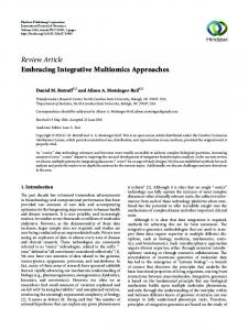


![Data Integration [PDF]](https://m.moam.info/img/260x300/data-integration-pdf_647aeb27098a9e06138b459c.jpg)


