Multi-particle dynamical systems and polynomials

Multi–particle dynamical systems and polynomials Maria V. Demina and Nikolai A. Kudryashov

arXiv:1407.1641v1 [nlin.SI] 7 Jul 2014

Department of Applied Mathematics National Research Nuclear University ”MEPhI” 31 Kashirskoe Shosse, 115409, Moscow, Russian Federation Abstract Polynomial dynamical systems describing interacting particles in the plane are studied. A method replacing integration of a polynomial multi–particle dynamical system by finding polynomial solutions of a partial differential equations is described. The method enables one to integrate a wide class of polynomial multi–particle dynamical systems. The general solutions of certain dynamical systems related to linear second–order partial differential equations are found. As a by-product of our results, new families of orthogonal polynomials are derived. Our approach is also applicable to dynamical systems that are not multi–particle by their nature but that can be regarded as multi–particle (for example, the Darboux–Halphen system and its generalizations). A wide class of two and three–particle polynomial dynamical systems is integrated.

Keywords: Multi–particle dynamical systems, polynomial solutions of partial differential equations, orthogonal polynomials

1

Introduction

Integrating an ordinary differential equation is one of the major problems of analysis. With the exception of certain classes of ordinary differential equations this problem is rather complicated. A. Cauchy suggested to study ordinary differential equations within the framework of complex analysis, what allowed him to obtain significant results on local existence and uniqueness of solutions. S.V. Kovalevskaya was one of the first mathematicians who noted a remarkable connection between explicit integrability of an ordinary differential equation and the singularity structure of its general solution [1,2]. Ideas of S.V. Kovalevskaya were extended and developed by E. Picard, G. Mittag–Leffler, P. Painlev´e, B. Gambier, F.J. Bureau. If the general solution of an ordinary differential equation does not have movable critical points, then it can be uniformized to fit the definition of a function (as a single valued mapping). Absence of movable critical points in the general solution of an ordinary differential equation is now called the Painlev´e property in honor of French mathematician P. Painlev´e. It can be concluded that an ordinary differential equation possessing the Painlev´e property is integrable in known functions or itself gives rise to a new function. L. Fuchs and H. Poincar´e suggested to look for new functions defined by ordinary differential equations. This problem can be solved in two steps. The first step is to make a classification of ordinary differential equations in a certain class, whose general solutions do not have movable critical points and, consequently, 1

define functions. The second step consists in selection of those equations that possess the general solutions not expressible via known functions. All linear equations generate functions. Nonlinear first–order algebraic ordinary differential equations give rise to only one new class of functions, the elliptic functions. A considerable contribution into the classification of second–order ordinary differential equations with the general solutions without movable critical points was done by P. Painlev´e. At the turn of the twentieth century the research group headed by P. Painlev´e performed the classification of second–order ordinary differential equations of the form wtt = R(wt , w, t),

(1.1)

where R is rational in wt and w [3, 4]. P. Painlev´e and his colleagues found fifty canonical equations with the general solutions possessing the Painlev´e property. Forty four equations can be integrated in terms of previously known functions and six equations required the introduction of new special functions. Nowadays these equations are called the Painlev´e equations and their general solutions are referred to as the Painlev´e transcendents. The complete list of equations (1.1) with the Painlev´e property can be found in [5]. The classification programm did not finish at second–order equations. J. Chazy made the classification of third–order ordinary differential equations in the polynomial class possessing the Painlev´e property [6]. J. Chazy considered equations in the form wttt = R(wtt , wt , w, t),

(1.2)

where R is a polynomial in wtt , wt , w. The work of J. Chazy was developed by F.J. Bureau, H. Exton, I. P. Martynov, C.M. Cosgrove, see [7] and references therein. The classification of ordinary differential equations is still going on. There exists a number of fourth and higher– order nonlinear equations that are supposed to define new functions [8–11]. However, this hypothesis is not proved yet [11]. The problem of integrating a system of nonlinear ordinary differential equations, especially if one can not obtain a single equation satisfied by some dependent function expressing all other functions from given equations, is even more difficult. In this article we consider systems of ordinary differential equations that can be regarded as multi–particle in the sense that given equations describe dynamics of point particles in the plane. Our aim is to integrate certain classes of multi–particle dynamical systems. Multi-particle dynamical systems, such as collections of interacting point vortices in the plane and on a sphere, have been attracting much attention during recent years. The point vortex system, an elegant and visual model of fluid dynamics, is not integrable in the case of four or more vortices with generic choice of circulations [12, 13]. That is why particular motions, including relative and absolute equilibria, collapse, and scattering are of great importance. A well–known class of absolute equilibria involving point vortices with equal in absolute value circulations is given by the roots of two neighbor Adler–Moser polynomials [14]. It is a remarkable fact that the roots of the Adler–Moser polynomials themselves provide solutions of another multi–particle system, the Airault–McKean–Moser dynamical system, related to the Korteweg – de Vries equation [15, 16]. Not long ago a method enabling one to find absolute and relative equilibrium configurations of point vortices in the plane and on a sphere was introduced and developed [17–24]. The starting point of the method is a polynomial or a system of polynomials with roots at the vortex positions. Further these polynomials are shown to obey certain ordinary differential equations. The strength of the method lies in the fact that it works in both directions: from, for example, point vortex relative equilibria to a differential equation and vice versa. In this article we generalize the polynomial method to the case of polynomial multi–particle dynamical systems. In fact, we shall study two problems. The first problem consists in finding 2

a dynamical system satisfied by the roots of a polynomial that obeys a partial differential equation. The second problem is opposite to the first. Suppose that one originates with a polynomial multi–particle dynamical system. The problem is to find a partial differential equation of degree less than the amount of particles such that the polynomial having roots coinciding with the particle positions in the plane satisfies this equation. The first problem has been considered previously (see [15, 25], works by F. Calogero [26, 27] and references therein). However, most of the authors deal with the case of rational solutions. In other words, there have been subsequent studies devoted to dynamical systems satisfied by the poles of rational solutions of integrable partial differential equations [15, 25–27]. While it seems that the second problem yet has not attracted any attention. Using the polynomial method we find solutions of some interesting dynamical systems related to linear second–order partial differential equations. As a byproduct of our results we derive new families of orthogonal polynomials. Our area of consideration includes not only dynamical systems multi–particle by their nature, but also systems that can be regarded as multi–particle. We integrate a wide class of two and three–particle polynomial dynamical systems. This class includes a number of systems interesting from physical point of view, such as the Euler’s and Darboux–Halphen systems. The Euler’s equations arise in rigid body dynamics. The Darboux–Halphen system finds applications in mathematical physics in relation to magnetic monopole dynamics, self–dual Einstein equations, topological field theory and in other fields of science [28–32]. Some generalizations of these systems also have a number of applications [32, 33]. For a class of two and three–particle polynomial dynamical systems including the aforementioned examples and their generalizations we present the cases, when such systems can be regarded as integrable in the sense that one can obtain their general solutions. For some other cases we give a number of exact elliptic solutions. In fact, we find all second–order elliptic solutions of a third–order differential equation arisen after application of the polynomial method. The problem of finding and classifying exact solutions of nonlinear ordinary and partial differential equations is of great theoretical and practical importance. In the past decades there has been a significant progress in the development of these methods. Group theoretical techniques provide exact solutions of equations possessing certain symmetries. Several powerful methods, such as the Hirota bilinear method, algorithms based on Darboux transformations and Wronskian representations, are designed mainly for partial differential equations integrable by inverse scattering method. An enormous number of methods deal with traveling wave solutions. Let us name only a few: the tanh–function method, the exponential method, the Jacobi elliptic– function method and their various extensions and modifications. Most of these methods use fixed expressions of unknown solutions. Consequently, all solutions lying outside supposed representations are lost. Along with this, such methods usually give the same solutions, but written in a different way. Consequently, this class of methods cannot be used if one wishes to perform a classification of exact solutions with given properties. In this article we shall use a method of finding exact elliptic solutions, which is free from these disadvantages. Our approach is based on Mittag–Leffler’s expansions of a meromorphic functions. This method allows one to find explicitly any elliptic solution of an algebraic ordinary differential equation. Consequently, the method can be used if one needs to classify elliptic solutions. This article is organized as follows. In section 2 we present our method and study the problem of finding dynamical systems related to polynomial solutions of partial differential equations. Section 3 is devoted to the problem of constructing a partial differential equation possessing polynomial solutions with the roots obeying a given polynomial multi–particle dynamical system. In section 4 we consider multi–particle dynamical systems related to linear second–order partial differential equations. In section 5 we study a class of two and three– particle polynomial dynamical systems, including physically meaningful ones. 3

2

Method applied

We begin with some preliminary remarks. Consider a polynomial in z with time–dependent coefficients: M −1 X M p(z, t) = c0 (t)z + cM −j (t)z j , c0 (t) 6≡ 0. (2.1) j=0

We suppose that the polynomial p(z, t) does not have multiple roots. This assumption gives a representation M Y p(z, t) = c0 (t) {z − aj (t)} , (2.2) j=1

where aj (t) 6≡ ak (t), j 6= k. Unless otherwise is stated, let z be a complex variable and let aj (t), cj (t) be complex–valued functions of a complex variable t. If we are interested in physically relevant solutions, then we shall restrict ourselves with real values of t. Calculating logarithmic derivatives of the polynomial p(z, t) yields relations M

M

pzz p2z X (−1) − 2 = 2, p p {z − a } j j=1

pz X 1 = , p z − a j j=1 and

M

X (−1)n+1 (n − 1)! dn log p = dz n {z − aj }n j=1

(2.3)

M


M ptz pt pz X −a2j,t − 2 = 2, p p {z − a } j j=1
M M 2 X (−aj,tt ) X −aj,t ptt p2t c0,tt c20,t − 2 = + − 2 + p p z − aj c0 c0 {z − aj }2 j=1 j=1

pt X (−aj,t ) c0,t + , = p z − a c j 0 j=1

(2.4)

For further convenience we introduce notation M X

Lm =

j=1,j6=k

1 , {ak − aj }m

Gm =

M X

j=1,j6=k

aj,t , {ak − aj }m

m ∈ N.

(2.5)

The derivatives of the function ak (t) and the quantities Lm , Gm can be expressed through the derivatives of the polynomial p(z, t). Let us consider in detail the derivation of ak,t , ak,tt , L1 . Multiplying the first relation in (2.4) by p and calculating the limit z → ak we easily get ak,t = −{pt /pz }z=ak . In order to find the limit in the right–hand side of the relation we have applied the l’Hˆopital’s rule. Since the polynomial p(z, t) does not have multiple roots, the following condition is valid {pz }z=ak 6≡ 0. Further, taking the second relation in (2.4) we find ak,tt {pz }z=ak = lim

z→ak

(p2t − ptt p) {z − ak }2 − a2k,t p {z − ak }2 p

=



2pt pz ptz − p2t pzz − p2z ptt p2z



.

(2.6)

z=ak

Let us calculate the quantity L1 . For this aim we take the first relation in (2.3), subtract from both sides the expression {z −ak }−1 and use the l’Hˆopital’s rule to obtain L1 = {pzz /(2pz )}z=ak . Analogously one can calculate higher–order derivatives of the function ak , if necessary, and quantities Lm , Gm . Let us write down those that we shall use later ak,t = −

pt , pz

pzz , L1 = 2pz

2pt ptz p2t pzz ptt pt pzz ptz c0,t − 3 − , G1 = − + , 2 pz pz pz 2p2z pz c0 pzzz p3zz p2 pzzzz pzz pzzz + . L2 = zz2 − , L3 = − 4pz 3pz 8pz 4p2z 8p3z ak,tt =

4

(2.7)

In expressions (2.7) all the derivatives of the polynomial p(z, t) are taken at its root ak . Obtained relations are of rather general character. They are valid for any polynomial with simple roots. Further let us note that any derivative of the polynomial p(z, t) at its root ak divided by (pz )z=ak can be expressed through the quantities ak,t , ak,tt , Lm , Gm (and their analogues arising in the case one wishes to find pttt , pzzt etc). Such relations can be obtained expressing step by step the corresponding derivatives from the equalities (2.7). For further purposes let us give several of them pt = −ak,t pz , ptz = −(G1 + ak,t L1 − {log c0 }t )pz , ptt = (2ak,t[G1 − {log c0 }t ] −ak,tt )pz , pzz = 2L1 pz , pzzz = 3(L21 − L2 )pz , pzzzz = 4(2L3 − 3L1 L2 + L31 )pz .

(2.8)

Here again all the derivatives of the polynomial p(z, t) are taken at its root ak . In addition we have M Y {ak − aj } {pz }z=ak = (2.9) j=1,j6=k

Now let us describe the polynomial method. In this section we shall mainly address the first problem from those stated in the introduction. Consider a partial differential equation E(t, z, pz , pt , ptz , ptt , pzz , . . .) = 0,

(2.10)

where E is a polynomial in z, p(z, t) and its derivatives. Here and in what follows we suppose that all the coefficient functions of partial differential equations and dynamical systems are well-behaved functions of the parameter t (i.e. entire or meromorphic). Suppose that a polynomial p(z, t) with simple roots solves this equation; then substituting z = ak and relations of the form (2.8) into equation (2.10), one obtains dynamical equations satisfied by the roots of the polynomial p(z, t). Thus the M zeros of the polynomial p(z, t) are interpreted as the coordinates of M point particles. The strength of the polynomial method lies in the fact that it enables one to restore original equation (2.10). Indeed, introducing a polynomial p(z, t) with the roots at particle positions and substituting equalities of the form (2.7) into the equations of motion and getting rid of the denominators, one arrives at the following relations {F (t, z, pz , pt , ptz , ptt , pzz , . . .)}z=ak = 0,

k = 1 . . . M,

(2.11)

where F is a polynomial in z, p, its derivatives and, consequently, a polynomial in z. This polynomial possesses M roots a1 , . . ., aM . Thus we conclude that F (t, z, pz , pt , ptz , ptt , pzz , . . .) − P (z, t)p = 0.

(2.12)

In this relation P (z, t) is a polynomial in z such that deg P = deg F − M. If deg F < M then P (z, t) ≡ 0. In nonlinear cases the polynomial P may depend on p(z, t) and its derivatives. At this step equation (2.12) may appear to be more general than the original equation (2.10). In other words, equations (2.10), (2.12) coincide accurate to the polynomial P (z, t). If we wish to identify the polynomial P (z, t) and to establish a correspondence between the polynomial solution p(z, t) of equation (2.10) and a dynamical system, then obtained dynamical equations may need additional constrains. In order to find them one can, for example, repeat the described procedure taking the differential consequences of original equation (2.10). The complete list of this constrains can be derived in the following way. Making the substitutions pz = up, pt = vp into equation (2.10) gives a partial differential equation with dependent variables p(z, t), u(z, t) and v(z, t) satisfying in addition the equation ut = vz . If p(z, t) is a polynomial with simple roots, then the functions u(z, t), v(z, t) are given by u(z, t) =

M X j=1

1 , z − aj

v(z, t) =

M X (−aj,t ) j=1

5

z − aj

+

c0,t . c0

(2.13)

Calculating the generalized Laurent series in a neighborhood of the pole ak for the functions u(z, t), v(z, t) yields ∞

X 1 (−1)m Lm+1 {z − ak }m , + u(z, t) = z − ak m=0

z → ak

(2.14)

∞

(−ak,t ) c0,t X v(z, t) = + + (−1)m+1 Gm+1 {z − ak }m , z − ak c0 m=0

z → ak .

The generalized Laurent series in a neighborhood of infinity are the following (M ) ∞ M X X m u(z, t) = aj z −m−1 , z → ∞ + z m=1 j=1 ( ) ∞ M c0,t X X − aj,t am z −m−1 , z → ∞. v(z, t) = j c0 m=0 j=1

(2.15)

Substituting series (2.14), (2.15), p(z, t) = {pz }z=ak (z − ak ) +

{pzz }z=ak (z − ak )2 + . . . + (z − ak )M , 2

z → ak ,

(2.16)

and relation (2.1), which is in fact the generalized Laurent series of the polynomial p(z, t) in a neighborhood of infinity, into the partial differential equation relating u, v, p and setting to zero the corresponding coefficients at negative and zero powers of {z − ak }, k = 1, . . ., M and z −1 gives the desired system. Indeed, the left–hand side of the equation relating u, v, p is a rational function without poles provided that this system is satisfied. From the Liouville theorem it immediately follows that such a function is a constant, which equals zero since the coefficients at zero powers of {z − ak }, k = 1, . . ., M, z vanish. Note that one may take only one correlation at the zero level {z − ak }0 , k = 1, . . ., M, z 0 . The coefficients {cm (t)} of the polynomial p(z, t) are expressible via the dynamical variables a1 (t), . . ., am (t) as follows cm = (−1)m Sm c0 ,

m = 1 . . . M,

(2.17)

where Sm are the elementary symmetric functions, see formulae (3.4) of section 3. As soon as the dynamical system is supplemented with additional constrains, then they can be used to identify the polynomial P (z, t) in (2.12). For this aim one rewrites these constrainers via {pz }z=ak , {pt }z=ak , etc., differentiates equation (2.12) with respect to z, and substitutes the corresponding derivatives expressed from the additional constrains into the resulting equation (see example below). For more details on constructing a partial differential equation related to a polynomial multi–particle dynamical system see section 3. Interestingly, the similar algorithm can be used to relate rational solutions of a partial differential equation and a dynamical system obeyed by the poles of its rational solutions. Let us consider several examples. It is known that the heat equation pt − pzz = 0.

(2.18)

possesses an infinite series of monic polynomial solutions, the so–called heat polynomials. Substituting relations (2.8) into equation (2.18) we immediately get ak,t = −2L1 or explicitly ak,t = −2

M X

1 , a k − aj j=1,j6=k 6

k = 1 . . . M.

(2.19)

If a starting point is the system (2.19) then introducing a monic polynomial p(z, t) with roots at the particle positions and using equalities (2.7) we obtain {pt − pzz }z=ak = 0.

(2.20)

The following inequality deg(pt − pzz ) < M is valid whenever p(z, t) is a monic polynomial. Consequently, the polynomial p(z, t) satisfies the heat equation. In addition, we see that system (2.19) does not need any additional constraint (with the only exception for initial conditions). If all the functions a1 (t), . . ., aM (t) are real then the corresponding system describes dynamics of identical point vortices on a line. As an illustrative nonlinear example let us take the following bilinear partial differential equation pptz − pz pt + ppzzzz − 4pz pzzz + 3p2zz = 0. (2.21)

Each polynomial from the sequence of the Adler–Moser polynomials is a monic polynomial solution of this equation. For some properties of the Adler–Moser polynomials see [15, 16, 34, 35]. Substituting relations (2.8) into equation (2.21) we obtain the following multi–particle dynamical equations M X 1 k = 1 . . . M. ak,t = −12 (2.22) 2, {a − a } k j j=1,j6=k

Our goal is to establish a correspondence between monic polynomials with simple roots that satisfy equation (2.21) and a dynamical system. Substituting pz = up, pt = vp into equation (2.21), we obtain ut + 6u2z + uzzz = 0. (2.23) Note that differentiating this equation with respect to z and introducing the new variable u˜ = 2uz yields the Korteweg – de Vries equation u˜t + 6˜ uu˜z + u˜zzz = 0.

(2.24)

Substituting series (2.14) into equation (2.23) and setting to zero coefficients at {z − ak }−2 and {z − ak }−1 gives (2.22) and constrains of the form M X

1 = 0, {ak − aj }3 j=1,j6=k

k = 1 . . . M.

(2.25)

An additional equation at the level z 0 is automatically satisfied. Originally dynamical system (2.22), (2.25) was found by Airault, McKean, and Moser [15]. Note that equations (2.22), (2.25) are compatible provided that M is a triangular number [15]. Now let us construct bilinear equation (2.21) originating from system (2.22), (2.25). Introducing a monic polynomial p(z, t) with roots at the particle positions and making use of relations (2.7) we get  pt pz + 4pz pzzz − 3p2zz z=a = 0, k = 1 . . . M; k  2 (2.26) 3 pz pzzzz − 2pz pzz pzzz + pzz z=a = 0, k = 1 . . . M. k

From the first set of these relations we obtain

pt pz + 4pz pzzz − 3p2zz − P (z, t)p = 0,

(2.27)

where P (z, t) is a polynomial in z of degree M − 2. Differentiating this equation with respect to z and setting z = ak yields {ptz pz + pt pzz + 4pz pzzzz − 2pzz pzzz − P (z, t)pz }z=ak = 0, 7

(2.28)

Our goal is to create an expression with a common multiplier pz . Consequently, we express pt from the first set of relations in (2.26) and find p3zz from the second set of relations in (2.26) and substitute the results into expressions (2.28) to obtain {[ptz + pzzzz − P (z, t)]pz }z=ak = 0,

(2.29)

The polynomial ptz + pzzzz − P (z, t) is of degree M − 2 and possesses M roots a1 , . . ., aM . Thus this polynomial identically equals zero and we conclude that P (z, t) = ptz + pzzzz .

(2.30)

This completes the derivation of equation (2.21). Finishing this section let us note that all our constructions are valid provided that aj (t) 6≡ ak (t), j 6= k. However, we do not exclude the cases when there exists an isolated point t = t0 such that aj (t0 ) = ak (t0 ). This coincidence gives rise to collisions of particles. In order to derive dynamical systems we perform the polynomial method in domains of the complex plane t, where aj (t) 6= ak (t) and further we use the principle establishing uniqueness of analytic continuation.

3

Polynomial multi–particle dynamical systems

In this section we shall originate with a multi–particle dynamical system and study the problem of finding a partial differential equation of degree less than the amount of particles such that the monic polynomial having roots coinciding with the particle positions in the plane satisfies this equation. Note that if a starting point is a multi–particle dynamical system, then we do not need to introduce non–monic polynomials. Let us consider the following dynamical system R(ak,tt , ak,t, ak ; a1 , . . . , ak−1 , ak+1 , . . . , aM ) = 0, k = 1 . . . M, (3.1) where the function R is a polynomial of its arguments with, possibly, t–dependent coefficients. In addition suppose that R is symmetric with respect to the variables a1 , . . ., ak−1 , ak+1 , . . ., aM . In the case ak 6≡ aj , k 6= j the system (3.1) can be regarded as a multi–particle dynamical system and the complex–valued functions a1 (t), . . ., aM (t) can be interpreted as particle positions in the plane. In what follows we shall call such a system polynomial multi– particle dynamical system. Note that we restrict ourselves we the first–order and second–order dynamical systems, since such systems are of great practical importance. While the polynomial method is applicable to polynomial multi–particle dynamical systems of arbitrary order. It is known that any symmetric polynomial of M − 1 variables a1 , . . ., ak−1 , ak+1 , . . ., aM can be represented as the polynomial in the following symmetric functions ′

sm =

M X

am j ,

j=1, j6=k

m ∈ N+

(3.2)

This representation is unique and involves finite amount of these functions. Let us introduce a monic polynomial p(z, t) with roots at the particle positions, see (2.1), (2.2) at cM (t) ≡ 1. Coefficients c1 , . . ., cM of the polynomial p(z, t) are symmetric polynomials with respect to the variables a1 , . . ., aM . Indeed, cm = (−1)m Sm ,

m = 1 . . . M,

(3.3)

where the elementary symmetric functions Sm are given by S1 = a1 + a2 + . . . + aM , S2 = a1 a2 + a1 a3 + . . . , S3 = a1 a2 a3 + a1 a2 a4 + . . . , SM = a1 a2 . . . aM 8

(3.4)

m In other words Sm is the sum of all CM products, containing m factors aj with distinct indices each. Equalities (3.3) should be replaced by (2.17) whenever one wishes to consider the non– monic case. It can be easily proved by induction that all the elementary symmetric functions S1 , . . ., SM can be expressed via ak and the derivatives  2   M −1    ∂ p ∂ p ∂p , , . . . , . (3.5) ∂z z=ak ∂z 2 z=ak ∂z M −1 z=ak

Calculating the z–derivatives of the polynomial p(z, t) and setting z = ak , we get  m  ∂ p (M − 1)! M! −m−1 akM −m + c1 aM + ... = k m ∂z (M − m)! (M − m − 1)! z=ak

(3.6)

+m!cM −m , m = 1 . . . M.

Relation (3.6) at m = M − 1 can be solved with respect to c1 . This gives  M −1  1 ∂ p c1 = − Mak . (M − 1)! ∂z M −1 z=ak Analogously, solving relation (3.6) at m = M − 2 with respect to c2 yields  M −2  1 ∂ p M(M − 1) 2 c2 = ak − (M − 1)ak c1 . − M −2 (M − 2)! ∂z 2 z=ak

(3.7)

(3.8)

Further, we substitute expression (3.7) into equality (3.8). We solve relation (3.6) at m = M −l with respect to cl . The coefficient cM is given by  M −1 cM = − aM + . . . + cM −1 ak . (3.9) k + c1 ak With the help of expressions (3.3), (3.6), (3.9) we can calculate all the functions S1 , . . ., SM . As soon as these functions are known, we use the Newton formulae sm − sm−1 S1 + sm−2 S2 − . . . + (−1)m−1 s1 Sm−1 + (−1)m mSm = 0, sm − sm−1 S1 + sm−2 S2 − . . . + (−1)M sm−M SM = 0,

m>M

1 ≤ m ≤ M;

(3.10)

to obtain the symmetric functions sm =

M X

am j ,

j=1

m ∈ N.

(3.11)

′

Consequently, the symmetric functions sm = sm − am k of M − 1 variables a1 , . . ., ak−1 , ak+1 , . . ., aM are polynomially expressible via ak and the derivatives (3.6). As we have already mentioned ′ dynamical equations (3.1) can be rewritten in terms of symmetric polynomials sm : ′ ˜ k,tt , ak,t, ak ; {sm R(a }) = 0,

k = 1 . . . M,

(3.12)

Substituting expressions of the form (3.7), (3.8) and relations for ak,t , ak,tt , see (2.6), into the resulting dynamical equations (3.12) and getting read of the denominators, we obtain the identities {F (t, z, p, pz , pt , . . .)}z=ak = 0, k = 1 . . . M, (3.13) 9

where F is a polynomial in z, p(z, t), its derivatives and, consequently, a polynomial in z with M roots a1 , . . ., aM . As a result we get the following partial differential equation F (t, z, p, pz , pt , . . .) − P (z, t)p = 0

(3.14)

with P being a polynomial in z of degree: deg P = deg F − M. The converse result is also valid. Suppose that we originate with a partial differential equation (3.14) and its polynomial solution p(z, t), see (2.2) with cM (t) ≡ 1. Setting z = ak in equation (3.14), we substitute relations (2.8) (also see expressions (3.3), (3.6)) into the resulting equality. This gives the symmetric dynamical system. The same approach is applicable to polynomial dynamical systems depending symmetrically not only on the variables a1 , . . ., ak−1 , ak+1 , . . ., aM but also on the variables a1,t , . . ., ak−1,t , ak+1,t , . . ., aM,t in such a way that the system can be rewritten in the form ˜ k,tt , ak,t , ak ; {s ′ }, {s ′ }) = 0, R(a m m,t

k = 1 . . . M,

(3.15)

′

In order to express the functions sm,t via ak , ak,t and the derivatives 

∂2 p ∂z∂t



z=ak

,



∂3 p ∂z 2 ∂t



,..., z=ak



∂M p ∂z M −1 ∂t



(3.16) z=ak

we consider the polynomial pt and calculate its z derivatives at the point z = ak  m+1  ∂ p (M − 1)! −m−1 = c1,t aM + . . . + m!cM −m,t , m = 0 . . . M. k m ∂z ∂t z=ak (M − m − 1)!

(3.17)

Further, we step by step express the quantities c1,t , . . ., cM,t from these relations and differentiate ′ the Newton formulae (3.10) to find sm,t and sm,t = sm,t − mam−1 ak,t . k Thus, the polynomial method enables one to place the study of polynomial multi–particle dynamical systems in the framework of the theory of partial differential equations. For a wide class of symmetric polynomial dynamical systems this approach yields only one ordinary differential equation for a certain coefficient of the polynomial p(z, t), see section 5. In this case the problem of integrating a symmetric polynomial dynamical system reduces to the problem of solving one ordinary differential equation and an M-th order algebraic equation. If a polynomial dynamical system with the dependent variables ξ = (ξ1 , . . . , ξM )T is not of multi–particle type, then one may look for an invertible transformation ξ = B(a) making the system in variables a = (a1 , . . . , aM )T symmetric as in (3.12) or (3.15). In conclusion let us mention that we have studied dynamical systems describing identical particle, i.e. particles possessing the same characteristics (such as mass, charge or circulation). The polynomial method is also applicable to systems of distinct particles. In the latter case one should divide the particles into groups according to the values of mass, charge, circulation etc. and introduce polynomials for each group separately [19–24]. Along with this it can be seen that polynomials with multiple roots satisfying partial differential equations give rise to dynamical systems describing behavior of distinct particles.

4

Multi–particle dynamical systems corresponding to linear partial differential equations

The polynomial method of solving a polynomial multi–particle dynamical system consists in finding polynomial solutions of the corresponding partial differential equation. In many cases 10

obtaining polynomial solutions of a linear partial differential equations is easier than those of nonlinear equations, especially at large values of the parameter M. In this section we shall construct and solve a number of multi–particle dynamical systems that originate from linear partial differential equations. Restricting ourselves with two–particle interactions (in the case M > 2) we consider second–order equations α0,2 (z, t)ptt + α0,1 (z, t)pt + α1,1 (z, t)ptz + α2,0 (z, t)pzz + α1,0 (z, t)pz + α0,0 (z, t)p = 0,

(4.1)

where the coefficient functions {α(z, t)} are polynomials in z. Suppose that a polynomial p(z, t) with simple roots is a solution of this equation. Substituting relations (2.8) into equation (4.1) gives the following multi–particle dynamical system α0,2 (ak , t)ak,tt + [α0,1 (ak , t) + 2α0,2 (ak , t){log c0 }t ] ak,t = α1,0 (ak , t) − α1,1 (ak , t){log c0 }t +

M X

1 {[2α0,2 (ak , t)ak,t − α1,1 (ak , t)]aj,t + [2α2,0 (ak , t) − α1,1 (ak , t)ak,t ]} , ak − aj j=1,j6=k

(4.2)

where k = 1 . . . M. Conversely, starting from system (4.2) we introduce a polynomial p(z, t) of degree M with roots at the particle positions (see (2.1)). By means of relations (2.7) we obtain equalities F [t, z, pz , pt , ptz , ptt , pzz ]z=ak = 0, k = 1 . . . M, where the polynomial F is given by F = α0,2 (z, t)ptt + α0,1 (z, t)pt + α1,1 (z, t)ptz + α2,0 (z, t)pzz + α1,0 (z, t)pz .

(4.3)

Thus we see that the polynomial p(z, t) satisfies the equation α0,2 (z, t)ptt + α0,1 (z, t)pt + α1,1 (z, t)ptz + α2,0 (z, t)pzz + α1,0 (z, t)pz − P (z, t)p = 0,

(4.4)

where P (z, t) is a polynomial in z of degree: deg P = deg F − M. Note that in the linear case the polynomial P does not depend on p and its derivatives. In order to identify P as α0,0 (z, t) system (4.2) should be supplied by additional constrains, which we derive as described in the previous section. This procedure is equivalent to substituting equality (2.1) into equation (4.1) and setting to zero the coefficients at z M +deg α0,0 , . . ., z M . A necessary and sufficient condition for a polynomial p(z, t) to satisfy equation (4.1) or (2.10) is existence of truncated Laurent series in a neighborhood of the points z = 0 and z = ∞. In fact, these series coincide and are given by (2.1). Substituting expression (2.1) into equation (4.1) and setting to zero coefficients at different powers of z one obtains a linear system for the coefficients c0 (t), . . ., cM (t). As a rule these equations are differential. As soon as a polynomial p(z, t) with simple roots that solves equation (4.1) is found it is an algebraic problem to obtain solutions of the corresponding dynamical system. Let us consider several examples. The following linear partial differential equation β2 ptt + β1 pt + σ(z)pzz + τ (z)pz + λp = 0

(4.5)

with β1 , β2 , λ being constants and σ(z), τ (z) being polynomials such that deg σ ≤ 2, deg τ ≤ 1 possesses stationary polynomial solutions given by classical orthogonal polynomials (of course, under appropriate choices of the parameter λ). Equation (4.5) necessarily admits polynomial solutions if the coefficient cM (t) satisfies the equation   M(M − 1) β2 c0,tt + β1 c0,t + σzz + Mτz + λ c0 = 0 (4.6) 2 This equation helps to find the polynomial P (z, t) in expression (4.4) and to establish a correspondence between polynomial solutions of equation (4.5) given by (2.2) and the following multi–particle dynamical system β2 ak,tt + [β1 + 2β2 {log c0 }t ]ak,t

M X β2 ak,t aj,t + σ(ak ) , = τ (ak ) + 2 a k − aj j=1,j6=k

11

k = 1 . . . M.

(4.7)

Hermite Laguerre Jacobi

Table 4.1: Classical orthogonal polynomials. pm (z) ρcop (z) [a, b] σ(z) Hm (z) exp(−z 2 ) (−∞, +∞) 1 (α) Lm (z), α > −1 z α exp(−z) [0, +∞) z (α,β) α β Pm (z), α > −1 (1 − z) (1 + z) [−1, 1] 1 − z2 β > −1

τ (z) −2z α+1−z β − α − (α +β + 2)z

λm 2m m m(m + α +β + 1)

By {pm (z)} we denote a sequence of classical orthogonal polynomials satisfying the equation σ(z)pm,zz + τ (z)pm,z + λm pm = 0 The polynomials {pm (z)} are orthogonal with respect to the weight function Z  τ 1 dz . ρcop (z) = exp σ σ

(4.8)

(4.9)

on the real interval [a, b], which may be infinite or half–infinite, see table 4.1. In these designations polynomial in z solutions of equation (4.5) can be presented in the form M X (4.10) p(z, t) = bm (t)pm (z), m=0

where the coefficients b0 (t), . . ., bM (t) satisfy the following linear ordinary differential equations β2 bm,tt (t) + β1 bm,t (t) + (λ − λm )bm = 0,

m = 0...M

Let us solve these equations. If β2 = 0, then we obtain   (λm − λ)t , m = 0 . . . M, bm (t) = Cm exp β1

(4.11)

(4.12)

where {Cm } are arbitrary constants. In the case β2 = 6 0 finding solutions of the quadratic equations β2 κ2 + β1 κ + (λ − λm ) = 0, m = 0 . . . M, (4.13) we get (2) κ(1) m 6= κm

(2) κ(1) m = κm (1)

⇒

⇒ (2)

(1) (2) (1) bm (t) = Cm exp[κ(1) m = 0...M m t] + Cm exp[κm t],  (1)  (2) (1) bm (t) = Cm + Cm t exp[κm t], m = 0 . . . M,

(4.14)

where again {Cm }, {Cm } are arbitrary constants. Stationary equilibria of dynamical system (4.7) is described by algebraic relations τ (ak ) + 2σ(ak )

M X

1 = 0, a k − aj j=1,j6=k

k = 1 . . . M.

(4.15)

The unique solution of this system is given by the roots of the classical orthogonal polynomial pM (z). Indeed, it follows from our results that the variables a1 , . . ., aM are solutions of this system if and only if the monic polynomial p(z) with roots at the points a1 , . . ., aM satisfies equation (4.8) with m = M. The unique (up to a constant multiplier, which does not affect the rools) polynomial solution of the latter equation is pM (z). Note that algebraic system (4.15) being considered in the complex plane possesses only real solutions. 12

Further let us study some other interesting examples involving classical orthogonal polynomials. It was proved in article [21] that the Wronskians P (z) = W [pi1 , . . . , pik , pik+1 ], Q(z) = W [pi1 , . . . , pik ], where i1 , . . . , ik+1 , k ∈ N+ is a sequence of pairwise different nonnegative integer numbers, satisfy the following equation     σz 1 σz {Px Q − P Qz } + {Px Q + P Qz } σ {Pzz Q − 2Px Qz + P Qzz } + τ + k − 2 2   (4.16) k(k − 1) + σzz + kτz + λik+1 P Q = 0. 2 In the case k = 0 we set P (z) = pi1 , Q(z) = 1. For further purposes we need the following theorem. Theorem 4.1. Neither the polynomials P (z) = W [pi1 , . . . , pik , pik+1 ], nor the polynomial Q(z) = W [pi1 , . . . , pik ] have common roots with the polynomial σ(z). Proof. First of all let us prove that if the polynomial Q(z) does not have common roots with the polynomial σ(z) then neither does the polynomial P (z). Suppose z = z0 is a root of the polynomial σ(z). Substituting the Tailor series in a neighborhood of the point z = z0 : σ(z) = σ1 (z − z0 ) + σ2 (z − z0 )2 , deg Q

Q(z) = κ0 +

X

m=1

m

κm (z − z0 ) ,

τ (z) = τ0 + τ1 (z − z0 ), deg P

r

P (z) = µr (z − z0 ) +

X

m=r+1

µm (z − z0 )m ,

(4.17)

where κ0 6= 0, µr 6= 0, r ∈ N+ , into equation (4.16) and setting the lowest–order coefficient to zero yields the equality rκ0 µr {(r + k − 1)σ1 + τ0 } = 0. (4.18) In the case of the Jacobi entries of the Wronskians we get z0 = 1, σ1 = −2, z0 = −1, σ1 = 2,

τ0 = −2(α + 1) ⇒ rκ0 µr {r + k + α} = 0, τ0 = 2(β + 1) ⇒ rκ0 µr {r + k + β} = 0.

(4.19)

From the conditions α > −1, β > −1 it follows that r = 0. In the case of the Laguerre entries of the Wronskians we have z0 = 0,

σ1 = 1,

τ0 = α + 1

⇒

rκ0 µr {r + k + α} = 0.

(4.20)

The condition α > −1 gives r = 0. Further we use induction over k. For k = 1, there is nothing to prove since the classical orthogonal polynomial pi1 does not have common roots with the polynomial σ(z). This completes the proof. Fixing the sequence i1 , . . . , ik let us consider the polynomials Pl (z) = W [pi1 , . . . , pik , pl ], l ∈ N+ \ I, I = {i1 , . . . , ik }. It turns out that such sequences of polynomials form orthogonal systems. Theorem 4.2. The polynomials Pl (z), l ∈ N+ \ {i1 , . . . , ik } are orthogonal with respect to the weight–function ρ˜(z) = (σ k ρcop )/q 2 on any simple directed smooth or piecewise smooth curve Γ with parametrization γ(s) : [sa , sb ] → C, [sa , sb ] ⊆ R provided that Γ avoids the zeros of the polynomial q(z) = W [pi1 , . . . , pik ], the integrals Z z n ρ˜(z)dz, n ∈ N+ (4.21) Γ

are finite, and the endpoints a = γ(sa ), b = γ(sb ) are chosen in such a way that lim ρ˜(γ(s))σ(γ(s))γ n (s) = 0,

s→sa +0

lim ρ˜(γ(s))σ(γ(s))γ n (s) = 0,

s→sb −0

13

n ∈ N+ .

(4.22)

Remark 1. In theorem 4.2 orthogonality is understood in the non–Hermitian sense Z Pl (z)Pn (z)˜ ρ(z)dz = 0, n 6= l

(4.23)

Γ

unless the curve Γ is an interval [a, b], possibly infinite or half–infinite, of the real line and ρ˜(z)dz is a positive measure on [a, b]. Remark 2. If the parameters α, β are not integers, then one should introduce cetrain cuts in the complex plane in order to ensure possibilities of choosing single valued branches of the functions z α , (1 − z)α , (1 + z)β . Remark 3. We do not exclude the case of closed curves, i.e. γ(sa ) = γ(sb ). For example, one can use this theorem to find polynomials orthogonal on a circle in the complex plane. Proof. We begin the proof by observing that substituting P = qψ, Q = q, ik+1 = l into expression (4.16) gives the following linear second order equation for the rational function ψ(z): σψl,zz + (τ + kσz ) ψl,z + (uk + λl ) ψl = 0,

(4.24)

where we have introduced notation uk (z) = kτz +

k(k − 1) σzz + σz {log q}z + 2σ{log q}zz . 2

(4.25)

Further using the standard technic designed for equations satisfied by the sequences of classical orthogonal polynomials we rewrite equation (4.24) in the form d (σρψl,z ) + (uk + λl ) ρψl = 0, dz

(4.26)

where the function ρ(z) is defined by the relation d (σρ) = (τ + kσz ) ρ. dz

(4.27)

Dividing this equality by σρ and integrating the result, we get ρ(z) = σ k ρcop . Multiplying equation by ψn , n 6= l yields (σρψl, z )z ψn + (uk + λl ) ρψl ψn = 0,

(4.28)

Reversing the subscripts, subtracting one equality from the other, and integrating the result gives  b Z W [Pn , Pl ] (4.29) , (λn − λl ) ψn (z)ψl (z)ρ(z)dz = − ρσ q2 Γ a

The path of integration Γ is chosen as given in the statement of the theorem. It follows from relations (4.22) that the right–hand side of expression (4.29) equals zero. Consequently, the sequence of rational functions ψl (z), l ∈ N+ \ {i1 , . . . , ik } is an orthogonal system with weight ρ(z) on the curve Γ. Recalling the definition of the function ψl (z), we obtain that the polynomials Pl (z), l ∈ N+ \ {i1 , . . . , ik } are orthogonal with weight ρ˜(z) = ρ(z)/q(z)2 on the curve Γ. This completes the proof. Polynomials, whose orthogonality we have proved in theorem 4.2, seem to belong to the class of exceptional orthogonal polynomials (for definitions and review of properties see [36, 37]). If the polynomial q(z) does not have real zeros, then the curve Γ in orthogonality condition (4.23) can be chosen as the real interval [a, b] and the endpoints may be taken as in the classical case. 14

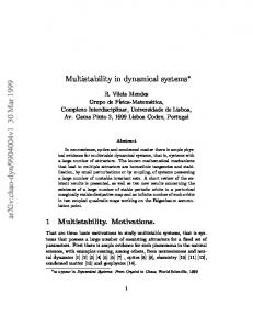
(a) q(z)

(b) P7 (z)

(c) P12 (z)

Figure 1: Roots of the polynomials q(z), {Pm (z)}, α = 2. The degrees of the polynomials Pl (z) = W [pi1 , . . . , pik , pl ], l ∈ N+ \ {i1 , . . . , ik }, q = W [pi1 , . . . , pik ] can be calculated finding the highest powers of the Wronskians. The result is k k X X k(k − 1) k(k + 1) (4.30) , deg q = im − . deg Pl = im + l − 2 2 m=1 m=1

Note that the following condition: deg Pl = l is valid not for all sequences of orthogonal polynomials. (α) (α) As an example let us take the Laguerre entries of the Wronskians. The polynomial W [L1 , L2 ] = −{z 2 − 2(α + 1)z + (α + 1)(α + 2)}/2 does not have real zeros provided that the inequality (α) (α) α > −1 is satisfied. Consequently, setting QL = W [L1 , L2 ] we obtain a family of poly(α) (α) (α) nomials P Lm = W [L1 , L2 , Lm ], m ∈ N+ \ {1, 2}, α > −1 orthogonal with the weight ρ˜(z) = (z α+2 exp[−z])/q 2 on the real interval [0, +∞): Z ∞ z α+2 e−z (4.31) dz = 0, n 6= l. P Ll (z)P Ln (z) QL2 0 According to relation (4.30) we have deg P Lm = m. Let us mention an interesting property of these polynomials. We observe that the polynomial P Lm (z) possesses m − deg QL simple zeros on the interval of orthogonality. For several plots see figure 1. Roots that are located on the curve of orthogonality are called regular. If the degrees of the polynomials in coefficients of equation (4.1) are the same as in expression (4.5), i.e. deg α0,2 = 0, deg α0,1 = 0, deg α0,0 = 0, deg α1,1 ≤ 1, deg α1,0 ≤ 1, deg α2,0 ≤ 2, then substituting equality (2.1) into equation (4.1) yields M + 1 linear second–order ordinary differential equations on M + 1 coefficients c0 (t), . . ., cM (t). In principle, these equations can be solved step by step (exact resolution, of course, depends on the functions of t involved in the coefficients {α(z, t)}). However, if the polynomials in coefficients of equation (4.1) are of higher degrees, then one obtains more than M + 1 equations on M + 1 coefficients c0 (t), . . ., cM (t). The problem to construct polynomial solutions of corresponding partial differential equations (or to prove their existence) becomes more complicated. As a result, it is not an easy task to find solutions of related dynamical systems (at least, by means of the polynomial method). We can use orthogonal polynomials Pl (z), l ∈ N+ \ {i1 , . . . , ik } to solve this problem whenever the z–part of a partial differential equation coincides with the equation for the system of orthogonal polynomials in question and α0,2 = β2 q, α0,1 = β1 q. 15

Polynomials with simple roots that solve the following linear partial differential equation  q{β2 ptt + β1 pt + σpzz } + [(τ + kσz )q − 2σqz ]pz + σqzz − (τ + (k − 1)σz )qz    (4.32) k(k − 1) σzz + kτz + λ q p = 0 + 2 give rise to the dynamical system of the form q(ak ) {β2 ak,tt + [β1 + 2β2 {log c0 }t ]ak,t } = 2q(ak )

M X β2 ak,t aj,t + σ(ak ) ak − aj

j=1,j6=k

+ {τ (ak ) + kσz (ak )} q(ak ) − 2σ(ak )qz (ak ),

(4.33)

k = 1 . . . M.

Suppose we wish to establish a correspondence between polynomials with simple roots that satisfy equation (4.32) and a dynamical system. It means that we should identify the polynomial P (z, t) in (4.4) as it is given in equation (4.32). For this aim we substitute expression (2.1) into equation (4.32) and set to zero the coefficients at different powers of z. We need to take equations at z M +deg q , . . ., z M . This gives additional constrains on dynamical variables a1 (t), (α) (α) . . ., aM (t). For example, in the case σ = z, τ = α + 1 − z, q = W [L1 , L2 ], k = 2 we obtain β2 c0,tt + β1 c0,t + (λ − M)c0 = 0, β2 c1,tt + β1 c1,t + (λ + 1 − M)c1 + δ2 c0 = 0, β2 c2,tt + β1 c2,t + (λ + 2 − M)c2 + δ3 c1 − 4(α + 1)Mc0 = 0

(4.34)

where δl = (M − l)2 + 2(M − l) + Mα. Further, we note that c1 = −{a1 + . . . + aM }c0 , c2 = {a1 a2 + a1 a3 + . . . + aM −1 aM }c0 , see also relations (2.17) in section 3. Equation (4.32) possesses polynomial solutions of the form p(z, t) =

M X

bm (t)Pm (z)

(4.35)

m=0, m6∈I

with coefficients bm (t), m ∈ N+ \ {I} given by (4.12), (4.14). Thus, we see that if such a polynomial does not have multiple roots, then these roots satisfy dynamical equations (4.33). We would like to remark that derived systems of orthogonal polynomials miss polynomials of certain degrees. Consequently, as soon as polynomial solution (4.35) is constructed one comes across a question whether expression (4.35) is the most general polynomial solution of partial differential equation (4.32). For certain systems of orthogonal polynomials including (α) (α) (α) the family P Lm = W [L1 , L2 , Lm ], m ∈ N+ \ {1, 2} we have checked that it is indeed the case. For this aim one can substitute the general expression for polynomial solutions (in terms of orthogonal polynomials under consideration and powers of z) into equation (4.32) and set to zero the corresponding coefficients. For example, in the case of the polynomials (α) (α) (α) P Lm = W [L1 , L2 , Lm ], m ∈ N+ \ {1, 2} we have substituted the following representation p(z, t) =

M X

bm (t)P Lm (z) + d2 (t)z 2 + d1 (t)z + d0 (t),

(4.36)

m=0, m6=1,2

where for d0 (t) we can take a partial solution of the corresponding ordinary differential equation. Further, we have shown that d2 (t) = 0, d1 (t) = 0, d0 (t) = 0.

16

5

Two and three–particle dynamical systems

In this section we consider the problem of integrating a class of two and three–particle polynomial dynamical systems. We begin with the two–particle non–autonomous dynamical systems given by a1,t = β1 (t)a21 + β2 (t)a22 + β3 (t)a1 a2 + β4 (t)a1 + β5 (t)a2 + β6 (t), a2,t = β1 (t)a22 + β2 (t)a21 + β3 (t)a1 a2 + β4 (t)a2 + β5 (t)a1 + β6 (t).

(5.1)

Let us suppose that the functions β1 (t), . . ., β6 (t) are entire or meromorphic. In order to apply the polynomial method we need the following relation: aj = {z − pz }x=ak , j 6= k. Applying the polynomial method we obtain the following partial differential equation pt + β2 p3z − {(2β2 + β3 )z + β5 }p2z + {(β1 + β2 + β3 )z 2 + (β4 + β5 )z + β6 (t)}pz −{f0 (t)z + f1 (t)}p = 0.

(5.2)

For subsequent convenience we introduce the new function: γ(t) = β1 (t) + β2 (t) − β3 (t). Substituting (2.1) with c0 (t) = 1, M = 2 into this equation yields the equalities f0 = 2γ, c2 =

f1 = (3β2 − β1 − β3 )w + 2(β4 − β5 ),

c1 = w,

1 {wt + (β2 + β1 )w 2 − (β4 + β5 )w + 2β6 (t)} 2γ

(5.3)

valid in the case γ 6≡ 0. Note that we do not exclude the situations, when the function γ(t) possesses isolated zeros. The function w(t) satisfies the following ordinary differential equation wtt + (4β1 − γ)wwt + {β1 − β2 }{2(β1 + β2 ) − γ}w 3 + {β5 − 3β4 − h}wt +{(β4 − β5 )γ + 4(β2 β5 − β1 β4 ) + (β1 + β2 )t − (β1 + β2 )h}w 2 + {2(β42 − β52 ) +4(β1 − β2 )β6 − (β4 + β5 )t + (β4 + β5 )h}w + 2{β0,t − h}β6 } + 4(β5 − β4 ) = 0,

(5.4)

where h(t) = (log γ)t . This equation belongs to the class of second–order differential equations studied by P. Painlev´e, B. Gambier, and their colleagues [3, 4], see the introduction. Consequently, if the functions β1 (t), . . ., β6 (t) are taken in such a way that equation (5.4) becomes one of the canonical equations found by P. Painlev´e and B. Gambier or is reducible to a canonical equation via the M¨obius transformation w(t) =

λ1 (t)W (t˜) + λ2 (t)W (t˜) , λ3 (t)W (t˜) + λ4 (t)W (t˜)

t˜ = Ψ(t),

λ1 λ4 − λ2 λ3 6= 0,

(5.5)

where Ψ(t), λj (t), j = 1 . . . 4 are locally analytic functions, then we conclude that polynomial solution (2.1) with c0 (t) = 1, M = 2 of equation (5.4) is constructed. The original dynamical system can be integrated finding the roots of the quadratic equation. For example, equation (5.4) coincides with the second Painlev´e equation wtt − 2w 3 − tw ±

1 =0 2

(5.6)

provided that the functions β1 (t), . . ., β5 (t) are constants and β2 = β1 ± 1,

β3 = −2β1 ± 1,

β4 = 0,

β5 = 0,

t β6 (t) = ± . 4

(5.7)

Note that the second Painlev´e equation in the form (5.6) possesses one–parametric family of exact solutions expressible via the Airy functions. Some exact solutions of equation (5.4) in autonomous case are given in article [38]. 17

If γ ≡ 0, then the functions f0 , f1 take the form f0 = 0,

f1 = 2(β2 − β1 )w + 2(β4 − β5 ).

(5.8)

The coefficient c1 = w satisfies the first–order ordinary differential equation wt + (β1 + β2 )w 2 − (β4 + β5 )w + 2β6 = 0,

(5.9)

which is linear whenever β1 ≡ −β2 and a Riccati equation in the case β1 6≡ −β2 . The coefficient c2 = y solves the following linear nonhomogeneous differential equation yt + 2{(β1 − β2 )w + β5 − β4 }y + β2 w 3 − β5 w 2 + β6 w = 0

(5.10)

Note that Riccati equation (5.9) is linearizable via the substitution w=

ψt , (β1 + β2 )ψ

β1 6= −β2

(5.11)

with the function ψ(t) satisfying the equation ψtt − {β4 + β5 + (log[β1 + β2 ])t }ψt + 2{β1 + β2 }β6 ψ = 0.

(5.12)

Further let us turn to a three–dimensional case. The following polynomial multi–particle dynamical system ak,t = β1

3 Y

aj + β2 ak

j=1,j6=k

+β5

3 X

aj + β3

j=1,j6=k

3 X

3 X

a2j + β4 a2k

j=1,j6=k

aj + β6 ak + β7 ,

(5.13)

k = 1, 2, 3

j=1,j6=k

contains as partial cases several systems of great practical importance. If β1 = 1, β2 = −1, and βj = 0, j = 2, . . ., 7 system (5.13) is exactly the classical Darboux–Halphen system ak,t =

3 Y

j=1,j6=k

aj − ak

3 X

aj ,

k = 1, 2, 3,

(5.14)

j=1,j6=k

which first appeared in Darboux’s works on triply orthogonal surfaces [28] and was later solved by Halphen [29, 30]. In successive studies, the classical Darboux–Halphen system has arisen as the Einstein field equations for a diagonal self–dual Bianchi–IX metric with Euclidean signature and in the similarity reductions of associativity equations on a three–dimensional Frobenius manifold [31]. The Euler’s dynamical system √ ξ1,t = σ1 ξ2 ξ3 + β6 ξ1 + σ1 β7 , √ ξ2,t = σ2 ξ1 ξ3 + β6 ξ2 + σ2 β7 , (5.15) √ ξ3,t = σ3 ξ1 ξ2 + β6 ξ3 + σ3 β7 , describing the rotation of a rigid body can be transformed into the multi–particle form ak,t = β1

3 Y

aj + β6 ak + β7 ,

j=1,j6=k

18

k = 1, 2, 3

(5.16)

√ √ √ by means of the transformation ξ = Ba with B = diag( σ1 , σ2 , σ3 ). In equations (5.16) we use the designation β1 = det B. Dynamical system (5.16) is also of the form (5.13). In order to apply the polynomial method to system (5.16) we need the following equalities 3 X



1 2z − pzz 2

3 Y





1 aj = aj = pz − zpzz + z 2 , 2 z=ak j=1,j6=k j=1,j6=k   3 X 1 2 2 2 aj = p − zpzz − 2pz + 2z . 4 zz z=ak j=1,j6=k



, z=ak

(5.17)

The polynomial method gives the partial differential equation of the form pt +

β3 1 pz p2zz − {(2β3 + β2 + β1 )z + β5 } pz pzz + {β1 − 2β3 }p2z + {(β1 + β4 4 2 +2β2 + 2β3 )z 2 + (2β5 + β6 )z + β7 }pz − {f0 (t)z + f1 (t)}p = 0.

(5.18)

We are interested in third–degree polynomials with simple roots that solve this equation. Substituting (2.1) with c0 (t) = 1, M = 3 into equation (5.18), we get relations f0 = 3(β1 + β4 − β2 − β3 ),

f1 = (β3 − β4 + 2β1 − 2β2 )c1 + 3(β6 − β5 )

(5.19)

and three equations for the coefficient functions c1 (t), c2 (t), c3 (t): c1,t + (2β3 + β4 )c21 − (2β5 + β6 )c1 + γ1 c2 + 3β7 = 0, c2,t + 2β3 c31 − 2β5 c21 + (β1 + β2 + β4 − 5β3 )c1 c2 + 2β7 c1 + 2(β5 − β6 )c2 + 3γ2 c3 = 0, c3,t + β3 c21 c2 − β5 c1 c2 + (2β2 + β4 − 2β1 − β3 )c1 c3 + (β1 − 2β3 )c22 + β7 c2 + 3(β5 − β6 )c3 = 0. (5.20) Here we have introduced notation γ1 = β1 + 2β2 − 2β4 − 4β3 , γ2 = β3 + β2 − β1 − β4 . If γ1 6≡ 0 and γ2 6≡ 0, then we solve the first equation with respect to c2 , the second equation with respect to c3 and substitute the resulting relations into the third equation. This yields the following third–order ordinary differential equation γ1 wttt + (δ1 w + δ5 )wtt + δ2 wt2 + (δ3 w 2 + δ6 w + δ7 )wt + δ4 w 4 +δ8 w 3 + δ9 w 2 + δ10 w + δ11 = 0.

(5.21)

for the function c1 = w. The coefficients of equation (5.21) are given in table 5.1. As soon as a solution w(t) of this equation is found, the coefficients c2 , c3 are polynomially expressible via w(t) and its derivatives. Again we do not exclude the situations, when the functions γ1 (t), γ2 (t) possess isolated zeros. Let us consider the case γ1 ≡ 0. If β4 ≡ −2β3 , then the first equation in (5.20) is linear, otherwise this equation is the Riccati equation linearizable via the substitution c1 =

ψt , (2β3 + β4 )ψ

β4 6= −2β3

(5.22)

with the function ψ(t) satisfying the equation ψtt − (2β5 + β6 )ψt + 3(2β3 + β4 )β7 ψ = 0.

(5.23)

Further, if γ2 6≡ 0, then solving the second equation in (5.20) with respect to c3 and substituting the result into the third equation, we obtain a second–order non-autonomous ordinary differential equation for the function c2 . If in addition to γ1 the coefficient γ2 identically equals zero, then the second equation in (5.20) is a first–order linear inhomogeneous equation. Solving 19

this equation we are left with the third equation in (5.20), which also becomes a first–order linear inhomogeneous equation. Ordinary differential equation (5.21) belongs to the class of third–degree equations studied by J. Chazy [6], see the introduction. In article [7] C.M. Cosgrove developed the works of J. Chazy and collected all third–order ordinary differential equations in polynomial class having the Painlev´e property. The general solutions of these equations are known. If the parameters of dynamical system (5.13) are taken in such a way that equation (5.21) is exactly one from those given in [7] or equation (5.21) is equivalent to one of the equations from article [7], then one can find the coefficient c1 (t) and, consequently, coefficients c2 (t), c3 (t). Thus we come to a conclusion that polynomial solution (2.1) with c0 (t) = 1, M = 3 of equation (5.18) is constructed. The original dynamical system can be integrated finding the roots of this polynomial. Recall that two equations in polynomial class are regarded as equivalent if their solutions w, w˜ are related via the transformation w(t) = λ0 (t)W (t˜) + λ1 (t), t˜ = Ψ(t). (5.24) In principle one may consider M¨obius transformation (5.5), but with possible loss of polynomial dependance of the function R in (1.2). It is an interesting fact that C.M. Cosgrove has also given a number of third–order equations of the form (5.21) that are not of Painlev´e–type but nevertheless that are integrable in the sense that one can find their general solutions [7]. Let us examine some interesting partial cases. In what follows we shall consider the autonomous case, i.e. we suppose that all the functions βj (t), j = 1, . . ., 7 are constants. Setting β2 = β1 , β3 = −β1 , β4 = −β1 , β1 6= 0 in (5.21) we obtain the linear third–order equation wttt + 3(β5 − 2β6 )wtt + (4β5 + 11β6 )(β6 − β5 )wt − 6{(2β5 + β6 )w − 3β7 }(β5 − β6 )2 = 0. (5.25) If all the parameters in (5.13) are chosen in such a way that system (5.13) becomes the classical Darboux–Halphen system (5.16), then the function y = 2w satisfies the Chazy-III equation yttt − 2yytt + 3yt2 = 0. (5.26) This equation is a famous Painlev´e–type equation admitting a movable natural barrier. Its general solution can be obtained inverting a hypergeometric function or using Schwarzian triangle functions [7]. Setting β3 = −(β1 + β2 )/2, β5 = 0, β6 = 0, β7 = 0 in equation (5.21), we see that the function y = −2(β4 + β2 )w, β2 6= −β4 satisfies the following third–order equation yttt − 2yytt + 3yt2 + σ(6yt − y 2)2 = 0,

σ=

(2β4 − β1 )2 − β2 (7β2 + 4β4 + 6β1 ) , 16(β2 + β4 )(3β1 − 2β4 + 4β2 )

(5.27)

which is the Chazy-XII equation if σ = 4/(n2 − 36), n ∈ N/{1, 6}. System (5.13) with β3 = −(β1 + β2 )/2, β5 = 0, β6 = 0, β7 = 0 can be regarded as a generalization of the classical Darboux–Halphen system. For details on the Chazy-XII equation see [7]. In the case of the Euler’s dynamical system (5.16) equation (5.21) takes the form wttt − (β1 w + 6β6 )wtt − 2β1 wt2 − (2β12 w 2 − 7β1 β6 w + 14β7 β1 − 11β62 )wt + 2β6 β12 w 3 −2β1 (2β62 + β7 β1 )w 2 + 6β6 (4β7 β1 − β62 )w + 18β7 (β62 − β7 β1 ) = 0.

(5.28)

The function y = −β1 w satisfies the Chazy-VII equation

yttt + yytt + 2yt2 − 2y 2yt = 0

(5.29)

provided that the parameters β6 , β7 vanish. The general solution of the Chazy-VII equation is known: y = {log ℘t (t − t0 ; g2, g3 )}t [7]. Here ℘(t − t0 ; g2, g3 ) is the Weierstrass elliptic function and t0 , g2 , g3 are arbitrary constants. 20

= γ31 (2γ1 + 5γ2 + 21β4 − 3β3 ) = 32 (γ12 + γ1 γ2 − 3γ22 ) + 2γ1 (β3 + 2β4 ) = 32 γ1 γ2 (2γ1 − γ2 ) + 18γ1 (β42 − β32 ) + 8γ2 (β4 γ1 − β3 γ2 ) + 4β4 (γ12 − γ22 ) + 4γ1 β3 (γ2 − γ1 ) = 32 (γ1 + 6β3 + 3β4 )(3γ1 {β3 − β4 }2 + 2γ1 γ2 {β3 − β4 } − 2β3 γ22 ) = 3γ1 (β5 − 2β6 ) − 2γ1,t − γ1 h2 (β5 − β6 )γ12 = 6γ1 {β3 + β4 }t − 3(β3 + 3β4 )γ1,t − 2γ1(β3 + 2β4 )h2 − 13 (2γ1 h2 + 5γ2 h1 ) + 10 3 − 13 (19β6 + 2β5 )γ1 γ2 + 4(2β5 + β6 )γ22 + ({22β5 − β6 }β3 + {8β5 − 29β6 }β4 )γ1 δ7 = −γ1,tt + (2h1 + h2 + 7β6 − β5 )γ1,t + (3β6 h2 − 2{2β6 + β5 }t )γ1 + 6β7 (γ1 − 6γ2 )γ2 +(β6 {11β6 − 7β5 } + 6β7 {β4 − β3 } − 4β52 )γ1 δ8 = 35 (2β3 + β4 )(3{β3 − β4 } − γ2 )γ1,t + 23 (β3 − β4 )(3{2β3 + β4 } + γ1 )γ1 h2 + 31 (2γ1 + 5γ2 −3β3 + 21β4 )γ1 β4,t + 32 (5γ2 − γ1 − 21β3 + 12β4 )γ1 β3,t + 23 (2β5 + β6 )(6β4 + 12β3 + γ1 )γ22 − 43 (β5 − β6 )(3{β3 − β4 } − γ2 )γ12 + 4({4β3 − β4 }β5 − {β3 + 2β4 }β6 )γ1 γ2 +18(β4 − β3 )(2β5 β3 − {β3 + β4 }β6 )γ1 δ9 = l(β + 2{ 13 (γ1 − 5γ2 ) + 7β3 − 4β4 }β5,t 3 , β4 ) + (2{7β5 − 4β6 }β3,t + {β5 − 7β6 }β4,t )γ1 1 +5  13 (2β5 + β6 γ2 ) + (β3 + 2β4 )β6 + (4β3 − β4 )β 5 γ1,t − { 3 (2γ1 + 5γ2 ) − β3 + 7β4 }β6,t 1 +2 3 (β5 − β6 )γ1 − (β3 + 2β4 )β6 + (4β3 − β4 )β5 γ1 h2 + 2(β5 − β6 )2 γ12 −2({2β5 + β6 }2 + {6(β4 + 2β3 ) + γ1 }β7 )γ22 + 4({β6 − β5 }{β6 + 2β5 } + 3{β4 − β3 }β7 )γ1 γ2 +18({β62 − β52 }β4 + {β3 − β4 }2 β7 + 2{β5 − β6 }β3 β5 )γ1 δ10 = l(β5 , β6 ) − 5β7 γ2 γ1,t + {2β52 − β62 − β5 β6 + 3(β3 − β4 )β7 }{5h1 + 2h2 }γ1 + {6(β4 − β3 )t β7 +2(4β6 − 7β5 )β5,t + (7β6 − β5 )β6,t + 5(γ2 − 3[β3 − β4 ])β7,t }γ1 + 12(2β5 + β6 )β7 γ22 −6(β5 − β6 )2 (2β5 + β6 )γ1 + 12(β5 − β6 )(3{β4 − β3 } + γ2 )β7 γ1 δ11 = 3β7,tt γ1 − 3β7 γ1,tt + 3(2h21 γ1 + h2 )β7 − 3(2γ1,t + γ1 h2 )β7,t + 6{β5 − β6 }t β7 γ1 +{β6 − β5 }{15(β7γ1,t − β7,t γ1 ) + 6β7 γ1 h2 } + 18({β5 − β6 }2 γ1 − β7 γ2 )β7 δ1 δ2 δ3 δ4 δ5 δ6

Table 5.1: Coefficients of equation (5.21). Designations: h1 = {log γ1 }t , h2 = {log γ2 }t , l(f, g) = {2f + g}tt γ1 + {(2h1 + h2 )γ1 h1 − γ1,tt }{2f + g} − {2f + g}t{2h1 + h2 }γ1 . Suppose that the present status concerning integrability of equation (5.21) at particular choice of the parameters is unknown; then one comes across a problem of finding some exact solutions. Let us derive certain well–behaved (meromorphic) exact solutions of equation (5.21). For this aim we shall use the method based on Mittag–Leffler’s expansions of meromorphic functions, see also [39–42]. In autonomous case equation (5.21) is invariant under the transformation t 7→ t − t0 , where t0 is an arbitrary parameter. Thus equation (5.21) may admit periodic meromorphic solutions. A single-valued function f (t) of one complex variable t is called meromorphic (in the complex plane) if it does not possess singularities in the finite points other than (isolated) poles. A meromorphic function holomorphic in the whole complex plane is entire. Any meromorphic functions is characterized by its behavior at infinity. There are three possibilities: (a) a point at infinity is a removable singularity or an (isolated) pole; (b) a point at infinity infinity is an (isolated) essential singularity; (c) a point at infinity infinity is a non–isolated singularity. In the case (a) the function f (t) is rational. In the case (b) the function f (t) is transcendental entire. Finally, in the remaining case (c) the function f (t) possesses infinitely many poles and is called transcendental meromorphic. The set of periods of a nonconstant meromorphic function f (t) is a discrete additive group: Ω = Z τ1 + Z τ2 . The parameters τ1 , τ2 are called fundamental (or principal) periods. If τ1 τ2 6= 0, then the meromorphic function is said to be doubly periodic (or elliptic). Note that the ratio τ1 /τ2 cannot be real. If one of the fundamental periods, for example, τ2 is zero, then the meromorphic function is said to be simply periodic. All the values an elliptic function takes in the parallelogram built on the periods τ1 , τ2 periodically arise in other point of the complex plane. The number of poles in a parallelogram 21

of periods, counting multiplicity, is called the order of an elliptic function. Analogously, behavior of a simply periodic meromorphic function in the complex plane is characterized by its behavior in a stripe built on the period τ1 . In what follows the fundamental period of a simply periodic meromorphic function we denote as T . Let us construct simply periodic meromorphic functions with one simple pole in a stripe of periods. Without loss of generality we place this pole at the origin. Using Mittag–Leffler’s expansions of meromorphic functions, we get  X  c−1 c−1 c−1 + h(t), + + f (t) = (5.30) t t − nT nT n∈Z, n6=0

where h(t) is a periodic entire function with the fundamental period T . Note that this function can be presented in the form   ∞ X 2πik t . h(t) = hk exp (5.31) T k=−∞ The series in expression (5.30) is uniformly convergent in any domain not including the points t = ZT . The constant term is added to each item in order to provide convergence. Implementing the summation yields   π πt f (t) = cot + h(t), (5.32) T T Calculating the derivative of expression (5.30) we find a simply periodic meromorphic function possessing (in a stripe of periods) one double pole with zero residue. In similar way we can construct simply periodic meromorphic functions with triple, etc pole in a stripe of periods. Any simply periodic meromorphic function with finite amount of poles b1 , . . ., bM in the fundamental stripe of periods is given by (M p )   (i) i π X X (−1)k−1 c−k dk−1 π{t − bi } (5.33) f (t) = + h(t), cot T i=1 k=1 (k − 1)! dtk−1 T where pi is the order of the pole z = bi and h(t) is again a periodic entire function. The simplest example of an elliptic function is the Weierstrass ℘–function defined as  X  1 1 1 ℘(t) = 2 + . − (5.34) t (t − nτ1 − mτ2 )2 (nτ1 + mτ2 )2 (n, m)6=(0, 0)

The series in expression (5.34) is uniformly convergent in any domain not including the points t = Zτ1 + Zτ2 . The Weierstrass elliptic function satisfies the following first–order ordinary differential equation (℘t )2 = 4℘3 − g2 ℘ − g3 . (5.35) Integrating the expression in (5.34), multiplying the result by −1 and using normalizing condition  Z 1 = 0. (5.36) ℘(t)dt + lim t→0 t

we obtain the Weierstrass ζ–function  X  1 1 t 1 ζ(t) = + + + . t t − nτ1 − mτ2 nτ1 + mτ2 (nτ1 + mτ2 )2 (n, m)6=(0, 0)

22

(5.37)

Note that the path of integration in (5.36) avoids the poles of ℘(t). Thus we see that ζt (t) = −℘(t). The Weierstrass ζ–function is not elliptic since the sum of the residues of any elliptic function at its poles in a fundamental parallelogram should be zero. But in combinations f (t) =

M X i=1

(5.38)

κi ζ(t − bi ) + h0

such that the condition κ1 + . . . + κM = 0 is satisfied the Weierstrass ζ–function produces an elliptic function with M simple poles in a parallelogram of periods: b1 , . . ., bM . Using expression (5.38) and the relation ℘(t) = −ζt (t) we can construct the general expression for an elliptic function with M poles in a parallelogram of periods. It is ) (M p M (i) i X XX (−1)k−1 c−k dk−1 (i) (5.39) ζ(t − b ) + h , c−1 = 0. f (t) = i 0 k−1 (k − 1)! dt i=1 i=1 k=1 Let us consider a nonlinear ordinary differential equation K[w(t)] = 0,

(5.40)

where the expression K[w(t)] is a polynomial in w(t) and its derivatives. Note that equation (5.21) in autonomous case is of the form (5.40). Behavior of a meromorphic function in a neighborhood of a pole can be characterized by means of its Laurent series. If one wishes to find its elliptic (5.43) or simply periodic (5.33) solutions explicitly it is necessary to construct families of Laurent series satisfying equation (5.40). For this aim the Painlev´e methods can be used. Taking equation (5.21) and applying these methods one can get (j)

w (t) =

pj X k=1

(j)

c−k {t − t0 }

k

+

∞ X k=0

(j)

ck {t − t0 }k ,

t → t0 ,

j ∈ J.

(5.41)

Here pi is the order of the pole t = t0 and the index j numerates different families of admissible series. The coefficients of the series can be sequently calculated, some of them may turn to be arbitrary. Note that particular series may exist under certain restrictions on the parameters of the original equation. Simply periodic solutions with finite amount of poles in a stripe of periods can be presented as follows o    n (j) Mj p j (j)   π t − bi π X X X (−1)k−1 c−k dk−1  + h(t),  (5.42) w(t) = cot T j⊆J  i=1 k=1 (k − 1)! dtk−1  T where T is the fundamental period, Mj is the number of poles of type j ⊆ J, and h(t) is a periodic entire function, see (5.31). The general expression for elliptic solutions is the following   Mj p j k−1  X X X (−1)k−1 c(j) (j) −k d w(t) = ζ(t − bi ) + h0 . (5.43) k−1  (k − 1)! dt  i=1 k=1 j⊆J

The theorem on total sum of the residues of any elliptic function gives a necessary condition for an elliptic solution to exist Mj XX (j) c−1 = 0. (5.44) j⊆J i=1

23

Note that we omit arbitrary constant t0 resulting from the invariance of equation (5.40) under the transformation t 7→ t − t0 . Further let us discuss the problem of finding solutions (5.42), (5.43) in explicit form. In this article we shall set h(t) = h0 in the case of simply periodic solutions (5.42), the possibility h(t) 6= h0 requires additional treatment. hFirst  of all letius mention that partial derivatives (j) of relations (5.43) are polynomials in cot π t − bi /T and elliptic functions, accordingly. Consequently, substituting relations (5.42), (5.43) into equation (5.40), we obtain a polynomial h   i (j) in cot π t − bi /T and an elliptic function, respectively. If the resulting function does no have poles, then from the Liouville theorem it immediately follows that such a function is a constant. Instead of substituting the solutions themselves we may substitute their Laurent (j) series in a neighborhood of the poles bi . Our algorithm can be subdivided into several steps. Step 1. Perform local singularity analysis for solutions of equation (5.40). Construct all the Laurent series of the form (5.41). Step 2. Write down general expressions (5.42), (5.43). Step 3. Take any solutions of step 2 and find its Laurent series in a neighborhood of the poles. Step 4. Substitute all those Laurent found at step 3 that are captured by a supposed solution into the n original o equation and set to zero coefficients at negative and zero powers of (j) the expression t − bi . Step 5. Solve obtained algebraic system. (j) As a rule, it is not an easy task to find h thei positions of the poles bi . It turns out that it is (j) (j) sufficient to obtain the values Bi = cot lbi , l = π/T in the case of simply periodic solutions (j)

(j)

(j)

(j)

and the values Ai = ℘(bi ; g2 , g3 ) and Bi = ℘t (bi ; g2 , g3 ) in the case of elliptic solutions (j) (j) instead. Note that the parameters Ai , Bi (in the elliptic case) are not independent, they are related by the equalities n o n o (j)

Bi

2

(j)

= 4 Ai

3

(j)

− g2 Ai − g3 .

(5.45)

Subsequently, addition formulae for periodic meromorphic functions can be used to rewrite solutions (5.42), (5.43) in terms of the new parameters, see [39–42]. As soon as a solution is found it is necessary to verify that its Laurent series in a neighborhood of different poles in the principle parallelogram of periods are in fact distinct. Now we pass on to finding well–behaved solutions of equation (5.21). In detail we shall consider the case of elliptic solutions only. If at least one of the parameters δ1 , δ2 , δ3 , δ4 is non–zero and some conditions on these parameters are satisfied, then equation (5.21) may have solutions with simple poles. Thus the simplest (second–order) elliptic solution is of the form ˜ 0, w(t) = c−1 ζ(t − t0 ; g2 , g3 ) − c−1 ζ(t − b − t0 ; g2 , g3 ) + h

(5.46)

˜ 0 are constants to be found, and t0 is an arbitrary constant resulting from where g2 , g3 , c−1 , h autonomy of equation (5.21). In what follows we omit this constant. Function (5.46) possesses two simple poles (t = 0 and t = b) in the principle parallelogram of periods. According to the preceding remarks we introduce the parameters: A = ℘(b; g2 , g3 ) and B = ℘t (b; g2 , g3 ) related by the equality B 2 = 4A3 − g2 A − g3 . Using addition formulae for the Weierstrass ζ–function, we rewrite relation (5.46) as follows w(z) = −

c−1 {℘t (t; g2 , g3 ) + B} + h0 , 2{℘(t; g2 , g3) − A} 24

˜ 0 + c−1 A. h0 = h

(5.47)

Let us turn to finding solutions (5.47) in explicit form. Substituting elliptic function (5.46) into equation (5.21), we get another elliptic function. If the resulting function does no have poles, it immediately follows that such a function is a constant since an elliptic function without poles does not exist. Instead of substituting the solution itself we shall substitute its Laurent series in a neighborhood of the poles t = 0, t = b. These Laurent series take the form  c−1 B 2 g2  3 c−1 t + ..., t → 0 + h0 + c−1 At − t + c−1 A2 − w(t) = t 2 10 c−1 c−1 B (5.48) w(t) = − + h0 − c−1 A{t − b} − {t − b}2 t−b 2  g2  {t − b}3 + . . . , t → b. −c−1 A2 − 10 In order to calculate these series we have used expression (5.46). Substituting series (5.48) into equation (5.21) we set to zero coefficients at negative and zero powers of t and t − b. We need only five first coefficients from each of the series. The resulting system contains nine equations including B 2 = 4A3 − g2 A − g3 . For all the solutions we find r δ6 4δ3 δ7 − δ62 6 (5.49) , g3 = 4A3 − g2 A − B 2 , A = , ε = ±1 c−1 = ε − , h0 = − δ3 2δ3 24δ3

and the following restrictions on the parameters of the original equation (4δ3 δ7 − δ62 )δ2 δ3 + 12(δ6 δ8 + 2δ4 δ7 )δ3 − 18δ4 δ62 , 8δ32 12δ8 δ3 − 18δ4 δ6 − δ2 δ3 δ6 3δ4 δ2 δ5 = , δ1 = − , δ3 6= 0. 2 4δ3 δ3 2

δ9 =

(5.50)

The first family exists under additional restrictions: δ2 = 0, δ4 = 0, δ8 = 0, δ10 = 0, δ11 = 0. In this case the parameters g2 , B are arbitrary and solution (5.47) is the general solution of the equation in question. For the second family we get δ2 = 0, δ4 = 0, δ10 = (3δ8 δ7 )/δ3 , δ8 6= 0. The parameter g2 is arbitrary and the parameter B is given by r 6 δ8 δ63 + 4δ11 δ33 − 2δ10 δ6 δ32 (5.51) B=ε − . δ3 144δ3 δ8 The third family exists provided that δ2 = 0, δ4 6= 0 and δ11

(2δ8 δ3 − 3δ4 δ6 )(2δ10 δ32 − 6δ8 δ7 δ3 + 9δ7 δ6 δ4 ) . = 4δ33 δ4

The parameter g2 is arbitrary and the parameter B takes the form r 6 (4δ10 δ3 − 12δ7 δ8 )δ32 + (δ62 + 12δ7 δ3 )δ4 δ6 . B=ε − δ3 144δ3 δ4

(5.52)

(5.53)

If the following conditions δ4 = −

δ2 δ3 , 2

δ10 =

(2δ2 δ6 + 3δ8 )δ7 , δ3

δ2 6= 0

(5.54)

are valid, then we obtain the fourth family of solutions. The parameter B is an arbitrary constant and the parameter g2 reads as r   6 (6δ7 δ3 − δ62 )δ8 δ6 − 2(δ2 δ72 + 2δ11 δ3 )δ32 + (6δ7 δ3 − δ62 )δ62 δ2 δ8 B+ε − g2 = δ6 + δ2 δ3 144δ2δ3 25

Finally, under the conditions δ2 6= 0, δ4 6= −(δ2 δ3 )/2 equation (5.21) possesses the fifth family of solutions with the parameters B and g2 given by r 6 (δ2 δ3 + 2δ4 )δ63 − 4(δ2 δ3 − 6δ4 )δ3 δ6 δ7 + 8(δ10 δ3 − 3δ7 δ8 )δ32 , B=ε − δ3 144(δ2 δ3 + 2δ4 )δ3 (5.55) (6δ4 − δ2 δ3 )(18δ4 + δ2 δ3 )δ7 δ62 + 4{µ2 δ3 − µ1 δ6 }δ3 , g2 = 48(δ2 δ3 + 2δ4 )δ32 δ2 where we have used notation µ1 = (δ2 δ3 − 6δ4 )δ3 δ10 + 2(18δ4 − δ2 δ3 )δ7 δ8 , µ2 = (δ2 δ3 + 2δ4 )(2δ3 δ11 + δ2 δ72 ) + 4(3δ8 δ7 − δ3 δ10 )δ8

(5.56)

Further, let us note that if δ3 = 0, δ4 = 0 and certain conditions on the parameters δ1 , δ2 , δ6 , δ8 are satisfied, then equation (5.21) may have solutions with second–order poles. Second–order elliptic functions having one double pole in the fundamental parallelogram of periods are the following w(z) = c−2 ℘(t − t0 ; g2 , g3 ) + h0 , (5.57) Without loss of generality, let us omit the arbitrary constant t0 . Finding the Laurent series of this function in a neighborhood of its pole t = 0, we obtain w(z) =

c−2 c−2 2 c−2 4 + h0 + g2 t + g3 t + . . . , 2 t 20 28

t→0

(5.58)

Here we have written down all the coefficients essential for further calculations. Substituting series (5.58) into equation (5.21) with δ3 = 0, δ4 = 0 and setting to zero the coefficients at negative and zero powers of t yields six families of solutions. For all the families the parameters c−2 , h0 are following 12 α7 c−2 = − , h0 = − , α6 6= 0. (5.59) α6 α6 Along with this we find two restrictions on the parameters of the original equation α8 =

α6 (2α2 + 3α1 ), 6

1 α9 = α5 α6 + (α1 + α2 )α7 . 2

(5.60)

The first family of solutions exists under additional constrains α2 6= 0, α1 6= −2α2 . The invariants g2 , g3 are given by α72 (α5 α7 − α10 )α6 + , g2 = 12 6(α1 + 2α2 )

α73 α62 α11 (α5 α6 + 2α2 α7 )(α5 α7 − α10 )α6 g3 = + + 216 144α2 144(α1 + 2α2 )α2

(5.61)

If α2 = 0, α1 6= 0, and α11 = (α10 − α5 α7 )α5 /α1 we obtain the second family of elliptic solutions with an arbitrary parameter g3 and the following value of the parameter g2 : α72 (α5 α7 − α10 )α6 + . g2 = 12 6α1

(5.62)

The third family of solutions exists whenever α1 = −2α2 , α2 6= 0, α10 = α5 α7 . In this case the parameter g2 is arbitrary and the parameter g3 is given by   1 α5 α6 α3 (2α6 α11 − α5 α72 )α6 (5.63) g3 = α7 + g2 − 7 + . 12 2α2 432 288α2

26

Further, if α1 = 0, α2 = 0, α10 = α5 α7 , α5 6= 0, then we obtain the fourth family of solutions with an arbitrary parameter g3 and the following value of the parameter g2 : α72 α6 α11 − . g2 = 12 6α5

(5.64)

Finally, under the restrictions α1 = 0, α2 = 0, α5 = 0, α10 = 0, α11 = 0 expression (5.57) is the general solution of the corresponding equation. In this case the invariants g2 , g3 are arbitrary, the third arbitrary constant is the parameter t0 . According to results of articles [39–42] we have classified all second–order elliptic solutions of equation (5.21). Note that in the case g23 − 27g32 = 0 elliptic solutions degenerate to simply periodic or rational. On use of obtained families of elliptic solutions one may construct exact solutions of the corresponding dynamical systems.

6

Conclusion

In this article we have considered polynomial multi–particle dynamical systems in the plane. We have presented a method, the polynomial method, which replaces integration of polynomial multi–particle dynamical systems by constructing polynomial solutions of partial differential equations. With the help of the polynomial method we have studied several interesting dynamical systems possessing equilibria given by the roots of classical and some other families of orthogonal polynomials. As a by–product of our results we have obtained several new families of orthogonal polynomials. We have integrated a wide class of two and three–particle polynomial dynamical systems including a number of physically relevant systems, such as, the Euler’s system, the Darboux– Halphen system, and their generalizations.

7

Acknowledgements

This research was partially supported by Russian Science Foundation, project to support research carried out by individual research groups No. 14-11-00258

References [1] Kowalevski S. Sur le probleme de la rotation d’un corps solide autour d’un point fixe, Acta Math. 12(1) (1889) 177–232. [2] Kowalevski S. Sur une propri´et´e du syst`eme d’´equations diff´erentielles qui d´efinit la rotation d’un corps solide autour d’un point fixe, Acta Math. 14(1) (1890-1891) 81–93. [3] Painlev´e P. Sur les ´equations diff´erentielles du second ordre et d’ordre superieur dont l’int´egrale g´en´erale est uniforme, Acta Math. 25(1) (1902) 1–85. [4] Gambier B. Sur les ´equations diff´erentielles du second ordre et du premier degr´e dont l’int´egrale g´en´erale est points critiques fixes, Acta Math. 33(1) (1910) 1–55. [5] Ince E. L. Ordinary differential equations (Longmans, Green, and co., London and New York, 1926). Reprinted (Dover, New York, 1956). Russian translation (GTIU, Khar’kov, 1939). 27

[6] Chazy J. Sur les ´equations diff´erentielles du troisi`eme et d’ordre sup´erieur dont l’int´egrale g´en´erale `a ses points critiques fixes, Acta Math., 34(1) (1911), pp. 317–385. [7] Cosgrove C.M. Chazy Classes IX–XI Of Third–Order Differential Equations, Studies in Applied Mathematics, 104(3) (2000) 171–228. [8] Airault H. Rational solutions of the Painlev´e equations, Stud. Appl. Math. 61 (1979) 31–53. [9] Flaschka H., Newell A.C. Monodromy- and spectrum-preserving deformations. I, Commun. Math. Phys. 76 (1980) 65–116. [10] Kudryashov N.A. The first and second Painlev´e equations of higher order and some relations between them, Phys Lett A 224 (1997) 353–360. [11] Kudryashov N.A. On the new transcendents defined by nonlinear ordinary differential equations, J. Phys. A.: Math. Gen. 31 (1998) L129. [12] Aref, H., Newton, P.K., Stremler, M.A., Tokieda, T., Vainchtein, D.: Vortex Crystals. Adv. Appl. Math. 39 (2003) 1–79. [13] Borisov A.V., Pavlov A.E. Dynamics and statics of vortices on a plane and a sphere - I, Regular and Chaotic Dynamics, 3 (1) (1998) pp. 28–38. [14] Bartman, A. B.: A new interpretation of the Adler–Moser KdV polynomials: interaction of vortices. In Nonlinear and turbulent processes in physics, vol. 3 (ed. R. Z. Sagdeev), pp. 11751181. New York, NY: Harwood Academic Publishers (1984). [15] Airault H., McKean H. P., and Moser J. Rational and elliptic solutions of the Korteweg de Vries equation and a related many-body problem, Comm. Pure Appl. Math. 30(1) (1977) 95-148. [16] Adler M., and Moser J. On a Class of Polynomials Connected with the KdV Equation, Commin. Math. Phys. 61 (1978) 1-30. [17] O’Neil K.A. Minimal polynomial systems for point vortex equilibria, Physica D, 219 (2006) 69 – 79. [18] Aref H. Relative equilibria of point vortices and the fundamental theorem of algebra, Proc. R. Soc. A., 467 (2011) 2168 – 2184. [19] Demina M.V., Kudryashov N.A. Point vortices and polynomials of the Sawada – Kotera and Kaup – Kupershmidt equations, R&C Dynamics, 16(6) (2011) 562-576. [20] Demina M.V., Kudryashov N.A. Vortices and polynomials: non–uniqueness of the Adler– Moser polynomials for the Tkachenko equation J. Phys. A: Math. Theor. 45 (2012) 195205. [21] Demina M.V., Kudryashov N.A. Point Vortices and Classical Orthogonal Polynomials, R&C Dynamics, 17(5) (2012) 371-384. [22] Demina M.V., Kudryashov N.A. Relative equilibrium configurations of point vortices on a sphere, R&C Dynamics, 18(4) (2013) 344–355. [23] Demina M.V., Kudryashov N.A. Polynomial Method for Constructing Equilibrium Configurations of Point Vortices in the Plane, Model. Anal. Inform. Sist. 47(7) (2013) 545–548. [24] Demina M.V., Kudryashov N.A. Rotation, collapse, and scattering of point vortices, Theoretical and Computational Fluid Dynamics, 28(3) (2014) 357–368. 28

[25] Choodnovsky D.V. and Choodnovsky G. V. Pole expansions of nonlinear partial differential equations, Nuovo Cimento B 40 (1977) 339-353. [26] Calogero F. Motion of poles and zeros of nonlinear and linear partial differential equations, and related solvable many-body problems, Nuovo Cimento B 43 (1978) 177-241. [27] Calogero F. Classical Many–Body Problems Amenable to Exact Treatments, Springer, Berlin, 2001. [28] Darboux G. Sur la th´eories des coordonn´eres curvilignes et les syst`emes orthogonaux, Ann. Ec. Normale Sup´er 7, 101–150 (1878). [29] Halphen G. Sur certains syst`emes d’´equations diff´erentielles, C. R. Acad. Sci. Paris 92, 1404–1406 (1881). [30] Halphen G. Sur syst`eme d’´equations diff´erentielles, C. R. Acad. Sci. Paris 92, 1101–1103 (1881). [31] Gibbons G. W. and Pope C. N. The positive action conjecture and asymptotically Euclidean metrics in quantum gravity, Commun. Math. Phys., 66 (1979), pp. 267–290. [32] Levi D., Ragnisco O. (Editors) SIDE III: Symmetries and Integrability of Difference Equations. American Mathematical Soc., 200– 444 p. [33] Ablowitz M.J., Chakravarty S., and Halburd R. The generalized Chazy equation and Schwarzian triangle functions, Asian J. Math. 2 (1998) 619–624. [34] Demina M.V., Kudryashov N.A.: Special polynomials and rational solutions of the hierarchy of the second Painlev´e equation. Theor. Math. Phys. 153(1) 1398–406 (2007) [35] Demina M.V., Kudryashov N.A.: The generalized Yablonskii–Vorob’ev polynomials and their properties. Phys. Lett. A. 372 (29) 4885–4890 (2008) [36] G´omez-Ullate D., Kamran N., Milson R. A Conjecture on Exceptional Orthogonal Polynomials, Foundations of Computational Mathematics 13(4) (2013) 615-666. [37] G´omez-Ullate D., Kamran N., Milson R. Exceptional orthogonal polynomials and the Darboux transformation, J. Phys. A: Math. Theor. 43 (2010) 434016. ′′

[38] Mittag–Leffler G. Sur l’int´egration de l’´equations diff´erentielles y = Ay 3 + By 2 + Cy + ′ D + (Ey + F )y (Extrait d’une lettre `a M. E. Picard) Acta Math. 18(1) (1894) 233–245. [39] Demina M.V., Kudryashov N.A. Explicit expressions for meromorphic solutions of autonomous nonlinear ordinary differential equations. Commun. Nonlinear Sci. Numer. Simulat. – 2011. – Vol. 16. P. 1127–1134. [40] Demina M.V., Kudryashov N.A. From Laurent series to exact meromorphic solutions: The Kawahara equation. Phys. Lett. A. – 2010. – Vol. 374. P. 4023–4029. [41] Demina M.V., Kudryashov N.A. On elliptic solutions of nonlinear ordinary differential equations. Appl. Math. and Comp. 2011. – Vol. 217 (23). P. 9849–9853. [42] Demina M.V., Kudryashov N.A. Elliptic solutions in the H´enon–Heiles model. Commun. Nonlinear Sci. Numer. Simulat. – 2014. – Vol. 19(3). P. 471–482.

29